
Mathematics is a big space of which humans so far have only charted a small amount. We know of countless areas in mathematics that we would like to visit, but that are not tractable computationally.
A prime reason Newtonian physics, as well as much of quantitative finance, is built around elegant but oversimplified models is that these models are easy to compute. For centuries, mathematicians have mapped small paths in the mathematical universe that they could travel down with a pen and paper. However, this all changed with the advent of modern high-performance computing. It unlocked the ability for us to explore wider spaces of mathematics and thus gain more accurate models.
In the final chapter of this book, you'll learn about the following:
- The empirical derivation of the Bayes formula
- How and why the Markov Chain Monte Carlo works
- How to use PyMC3 for Bayesian inference and probabilistic programming
- How various methods get applied in stochastic volatility models
This book has largely covered deep learning and its applications in the finance industry. As we've witnessed, deep learning has been made practical through modern computing power, but it is not the only technique benefiting from this large increase in power.
Both Bayesian inference and probabilistic programming are two up and coming techniques whose recent progress is powered by the increase in computing power. While the advances in the field have received significantly less press coverage than deep learning, they might be even more useful to the financial practitioner.
Bayesian models are interpretable and can express uncertainty naturally. They are less "black box," instead making the modeler's assumptions more explicit.
Before starting, we need to import numpy and matplotlib, which we can do by running the following code:
import numpy as np
import matplotlib.pyplot as plt% matplotlib inline
This example is similar to the one given in the 2015 book, Bayesian Methods for Hackers: Probabilistic Programming and Bayesian Inference, written by Cameron Davidson-Pilon. However, in our case, this is adapted to a financial context and rewritten so that the mathematical concepts intuitively arise from the code.
Note
Note: You can view the example at the following link: http://camdavidsonpilon.github.io/Probabilistic-Programming-and-Bayesian-Methods-for-Hackers/.
Let's imagine that you have a security that can either pay $1 or, alternatively, nothing. The payoff depends on a two-step process. With a 50% probability, the payoff is random, with a 50% chance of getting $1 and a 50% chance of making nothing. The 50% chance of getting the dollar is the true payoff probability (TPP), x.
This payoff scheme is visualized in the following diagram:
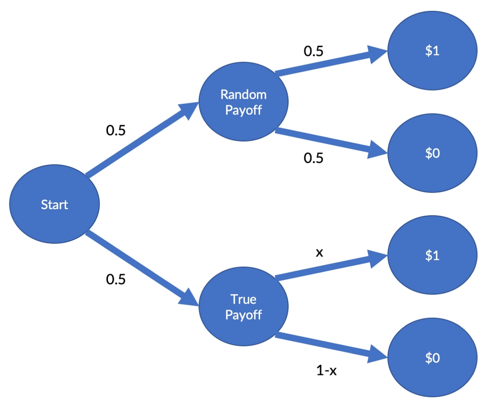
Payoff scheme
You are interested in finding out what the true payoff ratio is, as it will inform your trading strategy. In our case, your boss allows you to buy 100 units of securities. You do, and 54 of the 100 securities pay you a dollar.
But what is the actual TPP? In this case, there is an analytical solution to calculate the most likely TPP, but we will be using a computational method that also works for more complicated cases.
In the next section we will simulate the securities payoff process.
The variable x represents the TPP. We randomly sample 100 truth values, which are 1 if you had gotten the dollar under the true payoff, and 0 if otherwise. We also sample the two random choices at Start and Random Payoff in the preceding scheme. It is computationally more efficient to sample the random outcomes in one go for all trials, even though they are not all needed.
Finally, we sum up the payoffs and divide them by the number of securities in our simulation in order to obtain the share of payoffs in the simulation.
The following code snippet runs one simulation. It's important, though, to make sure that you understand how the computations follow from our securities structure:
def run_sim(x):
    truth = np.random.uniform(size=100) < x
    first_random = np.random.randint(2,size=100)
    second_random = np.random.randint(2,size=100)
    res = np.sum(first_random*truth + (1-first_random)*second_random)/100
    return res
Next, we would like to try out a number of possible TPPs. So, in our case, we'll sample a candidate TPP and run the simulation with the candidate probability. If the simulation outputs the same payoff as we observed in real life, then our candidate is a real possibility.
The following sample method returns real possibilities, or None if the candidate it tried out was not suitable:
def sample(data = 0.54):
    x = np.random.uniform()
    if run_sim(x) == data:
        return x
As we have to sample a number of possible TPPs, it's only natural that we want to speed this process up. To do this, we can use a library called JobLib, which will help with parallel execution.
Note
Note: JobLib is preinstalled on Kaggle kernels. For more information, you can visit https://joblib.readthedocs.io/en/latest/.
To do this, we need to import the Parallel class, which will help to run loops in parallel, and the delayed method, which helps to execute functions in order inside the parallel loop. We can import them by running the following:
from JobLib import Parallel, delayed
The details are not relevant for this example, but the Parallel(n_jobs=-1) method makes the job run with as many parallel executions as there are CPUs on the machine. For example, delayed(sample)() for i in range(100000) runs the sample method 100,000 times.
We obtain a Python list, t, which we turn into a NumPy array. As you can see in the following code snippet, about 98% of the array are None values. That means that 98% of the values the sampler tried out for x did not yield results matching our data:
t = Parallel(n_jobs=-1)(delayed(sample)() for i in range(100000))
t = np.array(t,dtype=float)
share = np.sum(np.isnan(t))/len(t)*100
print(f'{share:.2f}% are throwaways')
98.01% are throwaways
Therefore, we'll now throw away all of the None values, leaving us with the possible values for x:
t_flat = t[~np.isnan(t)]
plt.hist(t_flat, bins=30,density=True)
plt.title('Distribution of possible TPPs')
plt.xlim(0,1);
As a result of running this code, we'll get the following output:

Distribution of possible true payoff probabilities as found by our naïve sampler
As you can see, there is a distribution of possible TPPs. What this graph shows us is that the most likely TPP is somewhere around 50% to 60%; though other values are possible, they are somewhat less likely.
What you've just seen is one of the big advantages of Bayesian methods. All of the estimates come in distributions, for which we can then calculate confidence intervals, or credibility intervals, as they are known in Bayesian terminology.
This allows us to be more precise about how sure we are about things and what other values parameters in our model could have. Relating it back to our interest in finance, with financial applications, where millions are staked on the outputs of models, it becomes very advantageous to quantify such uncertainty.
At this point, you are able to take your results to your boss, who is a domain expert on the securities that you are trading. He looks at your analysis and shakes his head saying, "The TPP cannot be more than 0.5." He explains, "From the underlying business, it's physically impossible to do more than that."
So, how can you incorporate this fact into your simulation analysis? Well, the straightforward solution is to only try out candidate TPPs from 0 to 0.5. All you have to do is to limit the space you sample the candidate value of x, which can be achieved by running the following code:
def sample(data = 0.54):
    x = np.random.uniform(low=0,high=0.5)
    if run_sim(x) == data:
        return x
Now you can run the simulations exactly as before:
t = Parallel(n_jobs=-1)(delayed(sample)() for i in range(100000))
t = np.array(t,dtype=float)
# Optional
share = np.sum(np.isnan(t))/len(t)*100
print(f'{share:.2f}% are throwaways')
99.10% are throwaways
t_cut = t[~np.isnan(t)]
plt.hist(t_cut, bins=15,density=True)
plt.title('Distribution of possible TPPs')
plt.xlim(0,1);
Which, just like before, will give us the following output:

Distribution of possible TPPs from 0 to 0.5
Clearly, your choice of values to try influenced the outcome of your simulation analysis; it also reflected your beliefs about the possible values of x.
The first time around, you believed that all TPPs between 0 and 100% were equally likely before seeing any data. This is called a flat prior, as the distribution of values is the same for all values and is therefore flat. The second time, you believed that the TPPs had to be below 50%.
The distribution expressing your beliefs about x before seeing the data is called the prior distribution, P(TPP), or just prior. The distribution of the possible values of x that we obtained from simulation, that is, after seeing data D, is called the posterior distribution, ![]() , or just posterior.
, or just posterior.
The following plots show samples from prior and posterior for the first and second rounds. The first plot shows the results with a flat posterior:
flat_prior = np.random.uniform(size=1000000)
plt.hist(flat_prior,bins=10,density=True, label='Prior')
plt.hist(t_flat, bins=30,density=True, label='Posterior')
plt.title('Distribution of $x$ with no assumptions')
plt.legend()
plt.xlim(0,1);
This produces the following chart:

The results of our sampler with a flat prior
The next plot shows the output of our sampler with a <50% prior:
cut_prior = np.random.uniform(low=0,high=0.5,size=1000000)
plt.hist(cut_prior,bins=10,density=True, label='Prior')
plt.hist(t_cut, bins=15,density=True, label='Posterior')
plt.title('Distribution of $x$ assuming TPP <50%')
plt.legend()
plt.xlim(0,1);
While it's still the same sampler, you can see that the outcome is quite different:

The results of our sampler with a <50% prior
Have you noticed anything curious? The posterior values of the second round are roughly equal to the posterior values of the first round, but here they are cut off at 0.5. This is because the second round prior is 0 for values above 0.5 and 1 for everywhere else.
As we only keep simulation results that match the data, the number of kept simulation results shown in the histogram reflects the probability of running a simulation that yields the observed data D for a given TPP, C, ![]() .
.
The posterior probabilities, ![]() , that we obtain from our simulations are equal to the probability that we observe the data when trying out a given TPP,
, that we obtain from our simulations are equal to the probability that we observe the data when trying out a given TPP, ![]() , times the probability, P(TPP).
, times the probability, P(TPP).
Mathematically, this is represented as follows:

When the data is naturally obtained, such as through a face-to-face meeting, then we might need to account for biases in our data collection method. Most of the time, we do not have to worry about this and can simply leave it out, but sometimes the measurement can amplify certain outcomes.
To mitigate this, we'll divide by the data distribution, ![]() , as a final addon to our posterior formula and arrive at the following formula:
, as a final addon to our posterior formula and arrive at the following formula:

As you can see, it's the Bayes formula! When running our simulation, we are sampling from the posterior. So, why can't we just use the Bayes formula to calculate the posterior? The simple answer is because evaluating
requires integrating over TPP, which is intractable. Our simulation method is, as an alternative, a simple and convenient workaround.
In the previous section, we approximated the posterior distribution by randomly sampling from our prior and then trying out the sampled value. This kind of random trying works fine if our model only has one parameter, for example, the TPP. Yet, as our model grows in complexity and we add many more parameters, the random search method will become even slower.
Eventually, there will be too many possible parameter combinations that have no chance of generating our data. Therefore, we need to guide our search and sample parameters with higher posterior probabilities more often.
The approach of a guided, but still random, sampling is called the "Markov Chain Monte Carlo algorithm". The "Monte Carlo" component means that randomness and simulation are involved, whereas the "Markov Chain" means that we move over the parameter space under certain probabilities.
In the specific algorithm covered here, we will move to a different parameter value with a probability that is the ratio of the posterior probability of the parameter value. Here, we'll think of going to the posterior probability of the parameter value. As probabilities cannot be larger than one, we cap the ratio at one, but that is just a mathematical finite that does not matter much for the algorithm.
The following diagram shows the basic workings of the Markov Chain Monte Carlo algorithm:

The Markov Chain Monte Carlo algorithm
What the image shows is that we are on a "random walk" in which we more or less randomly go over different parameter values. However, we don't move entirely randomly, but instead prefer parameter values that have high posterior probabilities.
To execute this algorithm, we need to do four things:
-
Propose a new parameter value,
 , from our current parameter value, x.
-
Estimate the posterior probability of
 ,
,  . We can use the Bayes rule for this.
-
Calculate the probability,
 , of moving to that new parameter value,
  (remember that probabilities have to be smaller than one):

-
Move to the new parameter value with probability
 .
.
The next step is to build up these components step by step:
# REPETITION FROM FIRST SECTION
def run_sim(x):
    truth = np.random.uniform(size=100) < x
    first_random = np.random.randint(2,size=100)
    second_random = np.random.randint(2,size=100)
    res = np.sum(first_random*truth + (1-first_random)*second_random)/100
    return res
# REPETITION FROM FIRST SECTION
def sample(x,data = 0.54):
    if run_sim(x) == data:
        return x
First, we need to propose a new Xc. This has to be dependent on the previous value of x since we do not want a blind random search, but a more refined random walk. In this case, we will sample xcand from a normal distribution with mean x and a standard deviation of 0.1.
It's also possible to sample from other distributions or with other standard deviations, as long as xcand is related to x:
def propose(x):
    return np.random.randn() * 0.1 + x
In the first section, by sampling from the prior and then running the simulation, we sampled directly from the posterior. As we are now sampling through our proposed method, we are no longer sampling from the posterior directly. Therefore, to calculate the posterior probability, we'll use the Bayes rule.
Remember that we usually don't need to divide by P(D) as we don't assume biased measurements. The Bayes rule simplifies to  , where
  is the posterior, P(TPP) is the prior, and
  is the likelihood. So, to estimate the likelihood for a parameter value, x, we run a number of simulations with that parameter.
The likelihood is the share of simulations that match our data:
def likelihood(x):
    t = Parallel(n_jobs=-1)(delayed(sample)(x) for i in range(10000))
    t = np.array(t,dtype=float)
    return (1 - np.sum(np.isnan(t))/len(t))
For starters, we will use a flat prior again; each TPP is equally likely:
def prior(x):
    return 1 #Flat prior
The posterior probability of a parameter value, x, is the likelihood times the prior:
def posterior(x):
    return likelihood(x) * prior(x)
Now we are ready to put it all together into the Metropolis-Hastings MCMC algorithm!
First, we need to set some initial value for x. To make the algorithm find likely values quickly, it is sensible to initialize it at the maximum likelihood value or some estimate that we deem likely. We also need to compute the posterior probability of this initial value, which we can do by running the following code:
x = 0.5
pi_x = posterior(x)
Likewise, we need to keep track of all of the values sampled in a trace. Purely for exhibition purposes, we will also keep track of the posterior probabilities. To do this, we're going to run the following:
trace = [x]
pi_trace = [pi_x]
Now we get to the main loop. However, before we do, it's important to remember that the algorithm consists of four steps:
- Propose a new candidate xcand
- Compute the posterior probability of

- Compute the acceptance probability:

-
Set x to XC and with a probability,
 :
:
for i in range(1000): #Main Loop

    x_cand = propose(x)

    pi_x_cand = posterior(x_cand)

    alpha = np.min([1,pi_x_cand/(pi_x + 0.00001)]) # Save division

    u = np.random.uniform()

    (x, pi_x) = (x_cand,pi_x_cand) if u<alpha else (x,pi_x)
    trace.append(x)
    pi_trace.append(pi_x)

    if i % 10 == 0:
        print(f'Epoch {i}, X = {x:.2f}, pi = {pi_x:.2f}')
Epoch 0, X = 0.50, pi = 0.00Epoch 10, X = 0.46, pi = 0.04...Epoch 990, X = 0.50, pi = 0.06g
After running this algorithm for a number of epochs, we end up with a distribution of possible cheater shares with payoffs. As we've done before, we can simply run the following code to visualize this:
plt.hist(trace,bins=30)
plt.title('Metropolis Hastings Outcome')
plt.xlim(0,1);
Once we've run the previous code, we'll receive this graph as the output:

The outcome of the Metropolis Hastings sampler
By viewing the trace over time, it shows how the algorithm moves randomly but centers around highly likely values:
plt.plot(trace)
plt.title('MH Trace');
We will then get an output, in the form of a chart, which shows us the trace of the Metropolis Hasings (MH) sampler:

Trace of the Metropolis Hastings sampler
For a better understanding, we can plot the posterior probabilities over the tried out values:
plt.scatter(x=trace,y=pi_trace)
plt.xlabel('Proposed X')
plt.ylabel('Posterior Probability')
plt.title('X vs Pi');
After successful executing the code, we'll then get the following chart as an output:

The proposed value versus posterior probability
To demonstrate the power and flexibility of PyMC3, we are going to use it for a classic econometrics task, but we will put a Bayesian spin on it.
Note
Note: This example is a straight adaptation of an example from the PyMC3 documentation: https://docs.pymc.io/notebooks/stochastic_volatility.html. This, in turn, is an adaptation of an example from Hoffman's 2011 paper, No-U-Turn Sampler, available at: https://arxiv.org/abs/1111.4246.
Stock prices and other financial asset prices fluctuate, and the variance of daily returns is called volatility. Volatility is a commonly used risk measure, so it's quite important to measure it accurately.
The easy solution here would be to compute a backward-looking variance of return. However, there is a benefit to expressing uncertainty about the actual volatility. Similar to the payoff example we looked at earlier on, there is a distribution of "actual" values from which the realized values are drawn. This is also called "stochastic volatility" because there is a distribution of possible volatility values from which the observed volatility is a realized sample.
In this case we are interested in building a model of stochastic volatility of the S&P 500, the American stock market index. To do this, we must first load the data. You can either download them from Yahoo finance directly or find it on Kaggle, at https://www.kaggle.com/crescenzo/sp500.
To load the data, run the following code:
df = pd.read_csv('../input/S&P.csv')
df['Date'] = pd.to_datetime(df['Date'])
In the example we're looking at, we are interested in the closing prices, so we need to extract the closing prices from the dataset. The dataset shows new data first, so we need to invert it, which we achieve with the following code:
close = pd.Series(df.Close.values,index=pd.DatetimeIndex(df.Date))
close = close[::-1]
When plotting the closing prices, which we do in the following code, we see, through the outputted graphic, a familiar plot:
close.plot(title='S&P 500 From Inception');
SP500
As a result, we'll then get the following chart as an output:

The S&P 500 from inception to late 2018
The dataset contains the S&P since its inception, which for us is a bit too much, so in our case, we're going to cut it off at 1990. We can specify this date by running the following:
close = close['1990-01-01':]
As we are interested in the returns, we need to compute the price differences. We can use np.diff to get daily price differences. We are going to package the whole thing into a pandas series for easier plotting:
returns = pd.Series(np.diff(close.values),index=close.index[1:])
returns.plot();
This will give us the following chart:

The returns of the S&P 500 from 1990 to late 2018
Now the fun with PyMC3 begins. PyMC3 includes some special distributions for dealing with time series, such as a random walk. This is exactly the right thing to use when we want to model stock prices.
Firstly, we need to import PyMC3 and its tool for time series, the random walk class:
import pymc3 as pm
from pymc3.distributions.timeseries import GaussianRandomWalk
Then lastly, we need to set up the model. We can achieve this by running the following code:
with pm.Model() as model:
    step_size = pm.Exponential('sigma', 50.)      #1
    s = GaussianRandomWalk('s', sd=step_size,     #2
                           shape=len(returns))

    nu = pm.Exponential('nu', .1)                 #3

    r = pm.StudentT('r', nu=nu,                   #4
                    lam=pm.math.exp(-2*s),
                    observed=returns.values)
Let's now look at the commands we just executed in order to set up the model. As you can see, it consists of four key elements:
-
The volatility,
s, is modeled as a random walk with an underlying step size,step_size. Our prior for the step size is an exponential distribution with (once again, understanding the details of every distribution used is not necessary for the demonstration).
- We then model the stochastic volatility itself. Note how we plug in the step size, which is itself a random variable. The random walk should have the same length as the observed return values.
- We model the actual stock returns to be drawn from a
StudentTdistribution withnudegrees of freedom. Our prior fornuis an exponential distribution as well. - Finally, we get to model the actual returns. We model them to be drawn from a
StudentTdistribution with a scaling factor
(or
lamin code) produced by our stochastic volatile model. To condition the model on observed data, we pass on the observed return values.
The standard sampler for PyMC3 is not Metropolis Hastings, but the No-U-Turn Sampler (NUTS). PyMC3 will default to NUTS if we specify no sampler and just call sample.
To make the sampling run smoothly here, we need to specify a relatively high amount of tune samples. Those are samples that the sampler will draw from in order to find a good starting point, and that will not be part of the posterior, similar to the burned samples before.
We also need to tell NUTS to be lenient when accepting values by setting a high target_accept value. We can achieve this by running the following:
with model:
    trace = pm.sample(tune=2000, nuts_kwargs=dict(target_accept=.9))
PyMC3 has a nice utility that we can use to visualize the outcomes of sampling. We are interested in the standard deviation of the volatility random walk,  , as well as the degrees of freedom of the
 StudentT distribution from which the actual returns are drawn.
As we ran two chains in parallel, you can see that we obtained two different output distributions. If we had run the sampler for longer, those two outcomes would converge. We can obtain a better estimate by averaging them, which is what PyMC3 does for predictions. For instance, let's now try that with the following code:
pm.traceplot(trace, varnames=['sigma', 'nu']);
TracePlot
With the result of that code being shown in the following charts:

Results overview of the PyMC3 sampler. On the left, you can see the distributions produced by the two sampler chains. On the right, you can see their traces.
In the final step, we can show how stochastic volatility has behaved over time. You can see how it nicely aligns with volatile periods such as the 2008 financial crisis. You can also see that there are periods when the model is more or less certain about volatility:
plt.plot(returns.values)
plt.plot(np.exp(trace[s].T), 'r', alpha=.03);
plt.xlabel('time')
plt.ylabel('returns')
plt.legend(['S&P500', 'Stochastic Vol.']);
As we can see, the output of that code will return the chart that we see below:

Inferred stochastic volatility from 1990 to late 2018
There are a large number of applications that can be modeled well with such relatively small Bayesian models. The main advantage is that the models are easy to interpret and can express uncertainty well. Probabilistic programming aligns well with the "storytelling" approach to data science, as the story is clearly expressed in the model.
In the next section, we will move from shallow probabilistic programming to deep probabilistic programming.
The Bayesian models that we've developed so far are all quite shallow. So, let's ask ourselves whether we can combine the predictive power of deep networks with the advantages of Bayesian models. This is an active field of research and a fitting way to close this book.
Deep networks have a number of parameters; this makes searching through the parameter space a hard problem. In traditional supervised deep learning, we would use backpropagation to solve this problem. Backpropagation can also be used for Bayesian models. However, it's not the only, or even necessarily the best, way to do Bayesian deep learning.
By and large, there are four ways to do Bayesian deep learning:
- Use Automatic Differentiation Variational Inference (AVI). This means approximating the posterior with a guide model and then optimizing model parameters using gradient descent. PyMC3 can do this using the AVI optimizer. See the paper, Automatic Differentiation Variational Inference, by Alp Kucukelbir and others, 2016 paper at https://arxiv.org/abs/1603.00788.
- Alternatively, you can use, Pyro which implements fast, GPU-optimized AVI, which you can view here: http://pyro.ai/.
- While it would be too much to give an extensive tutorial on this approach here, the PyMC3 documentation has a good tutorial on this: https://docs.pymc.io/ notebooks/bayesian_neural_network_advi.html.
- Assume posterior values are normally distributed, then use a standard neural network library such as Keras and learn a mean and standard deviation for every parameter. Remember how we sampled the z value from a parameterized normal distribution when working on variational autoencoders? We can do this for every layer. This trains faster and takes less computing power and memory than AVI but is less flexible and has twice the parameters of a non-Bayesian neural network.
- Use the dropout trick. When working with time series, we turned dropout on at test time and ran inference multiple times to obtain confidence intervals. This is a form of Bayesian learning that is very easy to achieve, with no more parameters than a regular neural network. However, it's slower at inference time, and does not come with all the flexibility of AVI, either.
- Pick and mix. To train a neural network, we need a gradient signal, which we can obtain from AVI. We can train the socket of a neural network, sometimes called the feature extractor, in a regular fashion and the head of the network in a Bayesian manner. This way, we obtain uncertainty estimates while not having to pay the whole cost of Bayesian methods.