1

Introduction

During the years 1834 to 1845, Hamilton found a system of ordinary differential equations which is now called the Hamiltonian canonical system, equivalent to the Euler-Lagrange equation (1744). He also derived the Hamilton-Jacobi equation (HJE), which was improved/modified by Jacobi in 1838 [114, 130]. Later, in 1952, Bellman developed the discrete-time equivalent of the HJE which is called the dynamic programming principle [64], and the name Hamilton-Jacobi-Bellman equation (HJBE) was coined (see [287] for a historical perspective). For a century now, the works of these three great mathematicians have remained the cornerstone of analytical mechanics and modern optimal control theory.

In mechanics, Hamilton-Jacobi-theory (HJT) is an extension of Lagrangian mechanics, and concerns itself with a directed search for a coordinate transformation in which the equations of motion can be easily integrated. The equations of motion of a given mechanical system can often be simplified considerably by a suitable transformation of variables such that all the new position and momemtum coordinates are constants. A special type of transformation is chosen in such a way that the new equations of motion retain the same form as in the former coordinates; such a transformation is called canonical or contact and can greatly simplify the solution to the equations. Hamilton in 1838 has developed the method for obtaining the desired transformation equations using what is today known as Hamilton’s principle. It turns out that the required transformation can be obtained by finding a smooth function S called a generating function or Hamilton’s principal function, which satisfies a certain nonlinear first-order partial-differential equation (PDE) also known as the Hamilton-Jacobi equation (HJE).

Unfortunately, the HJE, being nonlinear, is very difficult to solve; and thus, it might appear that little practical advantage has been gained in the application of the HJT. Nevertheless, under certain conditions, and when the Hamiltonian (to be defined later) is independent of time, it is possible to separate the variables in the HJE, and the solution can then always be reduced to quadratures. In this event, the HJE becomes a useful computational tool only when such a separation of variables can be achieved.

Subsequently, it was long recognized from the Calculus of variation that the variational approach to the problems of mechanics could be applied equally efficiently to solve the problems of optimal control [47, 130, 164, 177, 229, 231]. Thus, terms like “Lagrangian,” “Hamiltonian” and “Canonical equations” found their way and were assimilated into the optimal control literature. Consequently, it is not suprising that the same HJE that governs the behavior of a mechanical system also governs the behavior of an optimally controlled system. Therefore, time-optimal control problems (which deal with switching curves and surfaces, and can be implemented by relay switches) were extensively studied by mathematicians in the United States and the Soviet Union. In the period 1953 to 1957, Bellman, Pontryagin et al. [229, 231] and LaSalle [157] developed the basic theory of minimum-time problems and presented results concerning the existence, uniqueness and general properties of time-optimal control.

However, classical variational theory could not readily handle “hard” constraints usually associated with control problems. This led Pontryagin and co-workers to develop the famous maximum principle, which was first announced at the International Congress of Mathematicians held in 1958 at Edinburgh. Thus, while the maximum principle may be surmised as an outgrowth of the Hamiltonian approach to variational problems, the method of dynamic programming of Bellman, may be viewed as an off-shoot of the Hamilton-Jacobi approach to variational problems.

In recent years, as early as 1990, there has been a renewed interest in the application of the HJBE to the control of nonlinear systems. This has been motivated by the successful development of the ${\mathcal{H}}_{\infty }$-control theory for linear systems and the pioneering work of Zames [290]. Under this framework, the HJBE became modified and took on a different form essentially to account for disturbances in the system. This Hamilton-Jacobi equation was derived by Isaacs [57, 136] from a differential game perspective. Hence the name Hamilton-Jacobi-Isaacs equation (HJIE) was coined, and has since been widely recognized as the nonlinear counterpart of the Riccati equations characterizing the solution of the ${\mathcal{H}}_{\infty }$-control problem for linear systems.

Invariably however, as in mechanics, the biggest bottle-neck to the practical application of the nonlinear equivalent of the ${\mathcal{H}}_{\infty }$-control theory [53, 138]-[145], [191, 263, 264] has been the difficulty in solving the Hamilton-Jacobi-Isaacs partial-differential equations (or inequalities); there is no systematic numerical approach for solving them. Various attempts have however been made in this direction with varying success. Moreover, recent progress in developing computational schemes for solving the HJE [6]-[10, 63] are bringing more light and hope to the application of HJT in both mechanics and control. It is thus in the light of this development that the author is motivated to write this book.

1.1    Historical Perspective on Nonlinear ${\mathcal{H}}_{\infty }$-Control

The breakthrough in the derivation of the elegant state-space formulas for the solution of the standard linear ${\mathcal{H}}_{\infty }$-control problem in terms of two Riccati equations [92] spurned activity to derive the nonlinear counterpart of this solution. This work, unlike earlier works in the ${\mathcal{H}}_{\infty }$-theory [290, 101] that emphasized factorization of transfer functions and Nevanlinna-Pick interpolation in the frequency domain, operated exclusively in the time domain and drew strong parallels with established LQG control theory. Consequently, the nonlinear equivalent of the ${\mathcal{H}}_{\infty }$-control problem [92] has been developed by the important contributions of Basar [57], Van der Schaft [264], Ball and Helton [53], Isidori [138] and Lin and Byrnes [182]-[180]. Basar’s dynamic differential game approach to the linear ${\mathcal{H}}_{\infty }$-control led the way to the derivation of the solution of the nonlinear problem in terms of the HJI equation which was derived by Isaacs and reported in Basar’s books [57, 59]. However, the first systematic solution to the state-feedback ${\mathcal{H}}_{\infty }$-control problem for affine-nonlinear systems came from Van der Schaft [263, 264] using the theory of dissipative systems which had been laid down by Willems [274] and Hill and Moylan [131, 134] and Byrnes et al. [77, 74]. He showed that, for time-invariant affine nonlinear systems which are smooth, the state-feedback ${\mathcal{H}}_{\infty }$-control problem is solvable by smooth feedback if there exists a smooth positive-semidefinite solution to a dissipation inequality or equivalently an infinite-horizon (or stationary) HJB-inequality. Coincidently, this HJB-inequality turned out to be the HJI-inequality reported by Basar [57, 59]. Later, Lu and Doyle [191] also presented a solution for the state-feedback problem using nonlinear matrix inequalities for a certain class of nonlinear systems. They also gave a parameterization of all stabilizing controllers.

The solution of the output-feedback problem with dynamic measurement-feedback for affine nonlinear systems was presented by Ball et al. [53], Isidori and Astolfi [138, 139, 141], Lu and Doyle [191, 190] and Pavel and Fairman [223]. While the solution for a general class of nonlinear systems was presented by Isidori and Kang [145]. At the same time, the solution of the discrete-time state and dynamic output-feedback problems were presented by Lin and Byrnes [77, 74, 182, 183, 184] and Guillard et al. [125, 126]. Another approach to the discrete-time problem using risk-sensitive control and the concept of information-state for output-feedback dynamic games was also presented by James and Baras [151, 150, 149] for a general class of discrete-time nonlinear systems. The solution is expressed in terms of dissipation inequalities; however, the resulting controller is infinite-dimensional. In addition, a control Lyapunov-function approach to the global output-regulation problem via measurement-feedback for a class of nonlinear systems in which the nonlinear terms depend on the output of the system, was also considered by Battilotti [62].

Furthermore, the solution of the problem for the continuous time-varying affine nonlinear systems was presented by Lu [189], while the mixed ${\mathcal{H}}_2$/${\mathcal{H}}_{\infty }$ problem for both continuous-time and discrete-time nonlinear systems using state-feedback control was solved by Lin [180]. Moreover, the robust control problem with structured uncertainties in system matrices has been extensively considered by many authors [6, 7, 61, 147, 148, 208, 209, 245, 261, 265, 284] both for the state-feedback and output-feedback problems. An inverse-optimal approach to the robust control problem has also been considered by Freeman and Kokotovic [102].

Finally, the filtering problem for affine nonlinear systems has been considered by Berman and Shaked [66, 244], while the continuous-time robust filtering problem was discussed by Nguang and Fu [210, 211] and by Xie et al. [279] for a class of discrete-time affine nonlinear systems.

A more general case of the problem though is the singular nonlinear ${\mathcal{H}}_{\infty }$-control problem which has been considered by Maas and Van der Schaft [194] and Astolfi [42, 43] for continuous-time affine nonlinear systems using both state and output-feedback. Also, a closely related problem is that of ${\mathcal{H}}_{\infty }$-control of singularly-perturbed nonlinear systems which has been considered by Fridman [104]-[106] and by Pan and Basar [218] for the robust problem. Furthermore, an adaptive approach to the problem for a class of nonlinear systems in parametric strict-feedback form has been considered again by Pan and Basar [219], while a fault-tolerant approach has also been considered by Yang et al. [285].

A more recent contribution to the literature has considered a factorization approach to the problem, which had been earlier initiated by Ball and Helton [52, 49] but discounted because of the inherent difficulties with the approach. This was also the case for the earlier approaches to the linear problem which emphasized factorization and interpolation in lieu of state-space tools [290, 101]. These approaches are the J-j-inner-outer factorization and spectral-factorization proposed by Ball and Van der Schaft [54], and a chain-scattering matrix approach considered by Baramov and Kimura [55], and Pavel and Fairman [224]. While the former approach tries to generalize the approach in [118, 117] to the nonlinear case (the solution is only given for stable invertible continuous-time systems), the latter approach applies the method of conjugation and chain-scattering matrix developed for linear systems in [163] to derive the solution of the nonlinear problem. However, an important outcome of the above endeavors using the factorization approach, has been the derivation of state-space formulas for coprime-factorization and inner-outer factorization of nonlinear systems [240, 54] which were hitherto unavailable [52, 128, 188]. This has paved the way for employing these state-space factors in balancing, stabilization and design of reduced-order controllers for nonlinear systems [215, 225, 240, 33].

In the next section, we present the general setup and an overview of the nonlinear ${\mathcal{H}}_{\infty }$-control problem in its various ramifications.

FIGURE 1.1
Feedback Configuration for Nonlinear ${\mathcal{H}}_{\infty }$-Control

1.2    General Set-Up for Nonlinear ${\mathcal{H}}_{\infty }$-Control Problems

In this section, we present a general framework and an overview of nonlinear ${\mathcal{H}}_{\infty }$-control problems using either state-feeback or output measurement-feedback. This setup is shown in Figure 1.1 which represents the general framework for ${\mathcal{H}}_{\infty }$-control problems. It shows the feedback interconnection of the plant P and the controller K with inputs w, u and outputs z, y. The plant can be described by a causal time-invariant finite-dimensional nonlinear state-space system P, with superscript “c” for continuous-time (CT) or “d” for discrete-time (DT), defined on a state-space $\mathcal{X}\subseteq {\Re }^n$ containing the origin x = {0}:

$CT:P^c:\{\begin{array}{l}\dot{x}=f\left(x,u,w\right),x\left(t_0\right)=x_0\\ y=h^y\left(x,w\right)\\ z=h^z\left(x,u\right)\end{array}$

(1.1)

$DT:P^d:\{\begin{array}{l}{x}_{k+1}=f\left(x_k,u_k,w_k\right),x\left(k_0\right)=x^0\\ y_k=h^y\left(x_k,w_k\right)\\ z_k=h^z\left(x_k,u_k\right),k\in Z\end{array}$

(1.2)

where $x\in \mathcal{X}$ is the state vector, $u:\Re \to \mathcal{U},w:\Re \to \mathcal{W}$ are the control input and the disturbance/reference signal (which is to be rejected/tracked) respectively, which belong to the sets of admissible controls and disturbances $\mathcal{U}\subset {\Re }^p,\mathcal{W}\subset {\Re }^r$ respectively, $f:\mathcal{X}\times \mathcal{U}\times \mathcal{W}\to \mathcal{X}$ is a smooth C^∞ vector-field (or vector-valued function), while $h^y:\mathcal{X}\times \mathcal{W}\to \mathcal{Y}\subset {\Re }^m,h^z:\mathcal{X}\times \mathcal{U}\to {\Re }^s$ are smooth functions. The output y ∈ $\mathcal{Y}$ is the measurement output of the system, while $z\in {\Re }^s$ is the controlled output or penalty variable which may represent tracking error or a fixed reference position. We assume that the origin x = 0 is an equilibrium-point of the system, and for simplicity f(0, 0, 0) = 0, h^z(0, 0) = 0.

We begin with the following definitions.

Definition 1.2.1 A solution or trajectory of the system P^c at any time t ∈ ℜ from an initial state x(t₀) = x₀ due to an input u[_t0 ,_t] will be denoted by x(t,t₀,x₀,u[_t0 ,_t]) or ϕ(t,t₀,x₀,u[_t0 ,_t]). Similarly, by x(k,k₀,x⁰,u[_k0 ,_k]) or ϕ(k₀,k,x⁰,u[_k0 ,_k]) for P^d.

Definition 1.2.2 The nonlinear system P^c is said to have locally ${\mathcal{L}}_2$-gain from w to z in $N\subset \mathcal{X}$, 0 ∈ N , less than or equal to γ, if for any initial state x₀ and fixed feedback u[_{t0 ,T}], the response z of the system corresponding to any w ∈ ${\mathcal{L}}_2$[t₀ ,T) satisfies:

${\displaystyle \underset{t_0}{\overset{T}{\int }}{\Vert z\left(t\right)\Vert }^{2}dt\le {\text{γ}}^2{\displaystyle \underset{t_0}{\overset{T}{\int }}{\Vert w\left(t\right)\Vert }^{2}dt}+\kappa \left(x_0\right),\forall T>t_0}$

for some bounded function κ such that κ(0) = 0. The system has ${\mathcal{L}}_2$-gain ≤ γ if $N=\mathcal{X}$.

Equivalently, the nonlinear system P^d has locallyℓ₂-gain less than or equal to γ in N if for any initial state x⁰ in N and fixed feedback u[_k0 ,_K], the response of the system due to any w[_k0 ,_K] ∈ℓ₂[k₀ ,K) satisfies

${\displaystyle \sum _{\kappa ={\kappa }_0}^K{\Vert z_{\kappa }\Vert }^2\le {\text{γ}}^2{\displaystyle \sum _{\kappa ={\kappa }_0}^K{\Vert w_{\kappa }\Vert }^2+\kappa \left(x^0\right),\forall K>{\kappa }_0,K\in Z}}\text{.}$

The system has ℓ₂-gain ≤ γ if $N=\mathcal{X}$.

Remark 1.2.1 Note that in the above definitions $\Vert .\Vert$ means the Euclidean-norm on ℜⁿ.

Definition 1.2.3 The nonlinear system P^c or [f,h^z] is said to be locally zero-state detectable in $\mathcal{O}\subset \mathcal{X}$,$0\in \mathcal{O}$, if w(t)≡ 0, u(t) ≡ 0, z(t) ≡ 0 for all t ≥ t₀, it implies lim_t→∞ x(t, t₀, x₀, u) = 0 for all $x_0\in \mathcal{O}$. The system is zero-state detectable if $\mathcal{O}=\mathcal{X}$ .

Equivalently, P^d or [f, h^y] is said to be locally zero-state detectable in $\mathcal{O}$ ifw_k ≡ 0, u_k ≡ 0, z_k ≡ 0 for all k ≥ k₀, it implies lim _k→∞ x(k, k₀, x⁰, u_k) = 0 for all $x^0\in \mathcal{O}$. The system is zero-state detectable if $\mathcal{O}=\mathcal{X}$.

Definition 1.2.4 The state-space $\mathcal{X}$ of the system P^c is reachable from the origin x = 0 if for any state x(t₁) ∈ $\mathcal{X}$ at t₁, there exists a time t₀ ≤ t₁ and an admissible control $u_{\left[t_0,t_1\right]}\in \mathcal{U}$ such that, x(t₁) = ϕ(t₁, t₀, {0},$u_{\left[t_0,t_1\right]}$] ).

Equivalently, the state-space of P^d is reachable from the origin x = 0 if for any state x_k1 ∈$\mathcal{X}$ at k₁, there exists an index k₀ ≤ k₁ and an admissible control $u_{\left[{\kappa }_0,{\kappa }_1\right]}\in \mathcal{U}$ such that, x_k1 = ϕ(k₁, k₀, {0}, u[_k0 ,_k1] ), k₀, k₁ ∈ Z.

Now, the state-feedback nonlinear ${\mathcal{H}}_{\infty }$-suboptimal control or local disturbance-attenuation problem with internal stability, is to find for a given number γ^⋆ > 0, a control action u = α(x) where α ∈ C^r(ℜⁿ), r ≥ 2 which renders locally the ${\mathcal{L}}_2$-gain of the system P from w to z starting from x(t₀) = 0, less or equal to γ^⋆ with internal stability, i.e., all state trajectories are bounded and/or the system is locally asymptotically-stable about the equilibrium point x = 0. Notice that, even though ${\mathcal{H}}_{\infty }$ is a frequency-domain space, in the time-domain, the ${\mathcal{H}}_{\infty }$-norm of the system P (assumed to be stable) can be interpreted as the ${\mathcal{L}}_2$-gain of the system from w to z which is the induced-norm from ${\mathcal{L}}_2$ to ${\mathcal{L}}_2$:

${\Vert P^c\Vert }_{\mathcal{H}\infty }=\underset{0\ne w\in {ℒ}_2\left(0,\infty \right)}{\sup }\frac{{\Vert z\left(t\right)\Vert }_2}{{\Vert w\left(t\right)\Vert }_2},x\left(t_0\right)=0,$

(1.3)

equivalently the induced-norm from ℓ₂ to ℓ₂:

${\Vert P^d\Vert }_{\mathcal{H}\infty }=\underset{0\ne w\in l_2\left(0,\infty \right)}{\sup }\frac{{\Vert z\Vert }_2}{{\Vert w\Vert }_2},x\left(k_0\right)=0,$

(1.4)

where for any v : [t₀, T ] ⊂ ℜ → ℜ^m or {v} : [k₀, K] ⊂ Z → ℜ^m,

${\Vert v\Vert }_{2\left[t_0,T\right]}^2\stackrel{\text{Δ}}{=}{\displaystyle \underset{t_0}{\overset{T}{\int }}{\displaystyle \sum _{i=1}^m\left|v_i{\left(t\right)}^2\right|dt,\text{and}{\Vert \left\{v_{\kappa }\right\}\Vert }_{2\left[{\kappa }_0,K\right]}^2}}\stackrel{\text{Δ}}{=}{\displaystyle \sum _{\kappa =k_0}^K{\displaystyle \sum _{i=1}^m{\left|v_{i\kappa }\right|}^2}}.$

The ${\mathcal{H}}_{\infty }$-norm can be interpreted as the maximum gain of the system for all ${\mathcal{L}}_2$-bounded (the space of bounded-energy signals) disturbances.

Thus, the problem can be formulated as a finite-time horizon (or infinite-horizon) minimax optimization problem with the following cost function (or more precisely functional) [57]:

$J^c\left(\mu ,w\right)=\underset{\mu \in \mathcal{U}}{\mathrm{min\hspace{0.17em}}}\underset{T}{\sup }\underset{w\in {ℒ}_2}{\sup }\frac{1}{2}{\displaystyle \underset{t_0}{\overset{T}{\int }}\left[{\Vert z\left(t\right)\Vert }^2-{\text{γ}}^2{\Vert w\left(t\right)\Vert }^2\right]d\tau ,T>t_0}$

(1.5)

equivalently

$J^d\left(\mu ,w\right)=\underset{\mu \in \mathcal{U}}{\mathrm{min\hspace{0.17em}}}\underset{T}{\mathrm{sup\hspace{0.17em}}}\underset{w\in l_2}{\sup }\frac{1}{2}{\displaystyle \sum _{k=k_0}^K\left[{\Vert z_k\Vert }^2-{\text{γ}}^2{\Vert w_k\Vert }^2\right],K>k_0\in \mathbf{\text{Z}}}$

(1.6)

subject to the dynamics P with internal (or closed-loop) stability of the system. It is seen that, by rendering the above cost function nonpositive, the ${\mathcal{L}}_2$-gain requirement can be satisfied. Moreover, if in addition, some structural conditions (such as observability or zero-state detectability) are satisfied by the disturbance-free system, then the closed-loop system will be internally stable [131, 268, 274].

The above cost function or performance measure also has a differential game interpretation. It constitutes a two-person zero-sum game in which the minimizing player controls the input u while the maximizing player controls the disturbance w. Such a game has a saddle-point equilibrium solution if the value-function

$V^c\left(x,t\right)=\underset{\mu \in \mathcal{U}}{\text{inf}}\underset{w\in {\mathcal{L}}_2}{\sup }{\displaystyle \underset{t}{\overset{T}{\int }}\left[{\Vert z\left(\tau \right)\Vert }^2-{\text{γ}}^2{\Vert w\left(\tau \right)\Vert }^{2}dt\right]}$

or equivalently

$V^d\left(x,k\right)=\underset{\mu \in \mathcal{U}}{\text{inf}}\underset{w\in l_2}{\sup }{\displaystyle \sum _{j=k}^K\left[{\Vert z_j\Vert }^2-{\text{γ}}^2{\Vert w_j\Vert }^2\right]}$

is C¹ and satisfies the following dynamic-programming equation (known as Isaacs’s equation or HJIE):

$\begin{array}{l}-V_t^c\left(x,t\right)=\underset{u}{\text{inf}}\underset{w}{\sup }\left\{V_x^c\left(t,x\right)f\left(x,u,w\right)+\left[\Vert z{\left(t\right)}^2\Vert -{\text{γ}}^2{\Vert w\left(t\right)\Vert }^2\right]\right\};\\ V^c\left(T,x\right)=0,x\in \mathcal{X},\end{array}$

(1.7)

or equivalently

$\begin{array}{l}{V}^d\left(x,k\right)=\underset{u_k}{\text{inf}}\underset{w_k}{\sup }\left\{v^d\left(f\left(x,u_k,w_k\right),k+1\right)+\left[\Vert z_k\Vert -{\text{γ}}^2{\Vert w_k\Vert }^2\right]\right\};\\ V^d\left(K+1,x\right)=0,x\in \mathcal{X},\end{array}$

(1.8)

where V_t, V_x are the row vectors of first partial-derivatives with respect to t and x respectively. A pair of strategies (μ^⋆, ν^⋆) provides under feedback-information pattern, a saddle-point equilibrium solution to the above game if

$J^c\left({\mu }^{\star },v\right)\le J^c\left({\mu }^{\star },v^{\star }\right)\le J^c\left(\mu ,v^{\star }\right)\text{,}$

(1.9)

or equivalently

$J^d\left({\mu }^{\star },v\right)\le J^d\left({\mu }^{\star },v^{\star }\right)\le J^d\left(\mu ,v^{\star }\right)\text{.}$

(1.10)

For the plant P, the above optimization problem (1.5) or (1.6) subject to the dynamics of P reduces to that of solving the HJIE (1.7) or (1.8). However, the optimal control u^⋆ may be difficult to write explicitly at this point because of the nature of the function f(., ., .).

Therefore, in order to write explicitly the nature of the optimal control and worst-case disturbance in the above minimax optimization problem, we shall for the most part in this book, assume that the plant P is affine in nature and is represented by an affine state-space system of the form:

$P^{ca}:\{\begin{array}{l}\stackrel{·}{x}=f\left(x\right)+g_1\left(x\right)w+g_2\left(x\right)u;x\left(0\right)=x_0\\ z=h_1\left(x\right)+k_{12}\left(x\right)u\\ y=h_2\left(x\right)+k_{21}\left(x\right)w\end{array}$

(1.11)

or

$P^{da}:\{\begin{array}{l}{x}_{k+1}=f\left(x_k\right)+g_1\left(x_k\right)w_k+g_2\left(x_k\right)u_k;x_0=x^0\\ z_k=h_1\left(x_k\right)+k_{12}\left(x_k\right)u_k\\ y_k=h_2\left(x_k\right)+k_{21}\left(x_k\right)w_k,k\in {\mathbf{Z}}_{+}\end{array}$

(1.12)

where $f:\mathcal{X}\to \mathcal{X},g_1:\mathcal{X}\to {ℳ}^{n\times r}\left(\mathcal{X}\right),g_2:\mathcal{X}\to {ℳ}^{n\times p}\left(\mathcal{X}\right),$, where ${ℳ}^{i\times j}\left(\mathcal{X}\right)$ is the ring of i × j matrices over $\mathcal{X},\text{while}{h}_1:\mathcal{X}\to {\Re }^s,h_2:\mathcal{X}\to {\Re }^m,$, and k₁₂, k₂₁ ∈ C^r, r ≥ 2 have appropriate dimensions.

Furthermore, since we are more interested in the infinite-time horizon problem, i.e., for a control strategy such that ${\lim }_{T\to \infty }{J}^c\left(u,w\right)\left(\text{resp}\text{.}{\text{lim}}_{K\to \infty }{J}^d\left(u_k,w_k\right)\right)$ remains bounded and the ${\mathcal{L}}_2$-gain (resp. ℓ₂-gain) of the system remains finite, we seek a time-independent positive-semidefinite function $V:\mathcal{X}\to \Re$ which vanishes at x = 0 and satisfies the following time-invariant (or stationary) HJIE:

$\begin{array}{l}\underset{\mu }{\mathrm{min\hspace{0.17em}}}\underset{w}{\sup }\left\{V_x\left(x\right)\left[f\left(x\right)+g_1\left(x\right)w\left(t\right)+g_2\left(x\right)u\left(t\right)\right]+\frac{1}{2}\left({\Vert z\left(t\right)\Vert }^2-{\text{γ}}^2{\Vert w\left(t\right)\Vert }^2\right)\right\}=0;\\ V\left(0\right)=0,x\in \mathcal{X}\end{array}$

(1.13)

or equivalently the discrete HJIE (DHJIE):

$\begin{array}{l}V\left(x\right)=\underset{\mu }{\mathrm{min\hspace{0.17em}}}\underset{w}{\sup }\left\{V\left(f\left(x\right)+g_1\left(x\right)w+g_2\left(x\right)u\right)+\frac{1}{2}\left({\Vert z\Vert }^2-{\text{γ}}^2{\Vert w\Vert }^2\right)\right\}=0;\\ V\left(0\right)=0,x\in \mathcal{X}.\end{array}$

(1.14)

The problem of explicitly solving for the optimal control u^⋆ and the worst-case disturbance w^⋆ in the HJIE (1.13) (or the DHJI (1.14)) will be the subject of discussion in Chapters 5 and 7 respectively.

However, in the absence of the availability of the state information for feedback, one might be interested in synthesizing a dynamic controller K which processes the output measurement y(t), t ∈ [t₀, T ] ⊂ [0,∞) (equivalently y_k, κ ∈ [k₀, K] ⊂ [0, ∞)) and generates a control action u = α([t₀, t]) (resp. u = α([k₀, k])) that renders locally the ${\mathcal{L}}_2$-gain (equivalently ℓ₂-gain) of the system about x = 0 less than or equal to γ > 0 with internal stability. Such a controller can be represented in the form:

$\begin{array}{l}{K}^c:\dot{\xi }=\eta \left(\xi ,y\right),\xi \left(0\right)={\xi }_0\\ u=\text{θ}\left(\xi ,y\right)\end{array}$

$\begin{array}{l}{K}^d:{\xi }_{\kappa +1}=\eta \left({\xi }_{\kappa },y_{\kappa }\right),{\xi }_0={\xi }^0\\ u_{\kappa }=\text{θ}\left({\xi }_{\kappa },y_{\kappa }\right),k\in Z_{+},\end{array}$

where $\text{ξ}\text{:}[0,\infty )\to \mathcal{X},\eta :\mathcal{O}\times \mathcal{Y}\to \mathcal{X},\theta :\mathcal{O}\times \mathcal{Y}\to {\Re }^p$. This problem is then known as the suboptimal local ${\mathcal{H}}_{\infty }$-control problem (or local disturbance-attenuation problem) with measurement-feedback for the system P. The purpose of the control action is to achieve local closed-loop stability and to attenuate the effect of the disturbance or reference input w on the controlled output z.

Often this kind of controller will be like a carbon-copy of the plant which is also called observer-based controller, and the feedback interconnnection of the controller K and plant P results in the following closed-loop system:

$P^{ca}\circ K^c:\{\begin{array}{l}\dot{x}=f\left(x\right)+g_1\left(x\right)w\left(x\right)+g_2\left(x\right)\theta \left(\xi ,y\right);x\left(0\right)={\widehat{x}}_0\\ \xi =\eta \left(\xi ,y\right),\xi \left(0\right)={\xi }_0\\ z=h_1\left(x\right)+k_{12}\left(x\right)\theta \left(\xi ,y\right)\\ y=h_2\left(x\right)+k_{21}\left(x\right)w\left(t\right)\end{array},$

(1.15)

or equivalently

$P^{da}\circ K^d:\{\begin{array}{l}{x}_{k+0}=f\left(x_k\right)+g_1\left(x_k\right)w_k+g_2\left(x_k\right)\theta \left({\xi }_k,y_k\right);x_0=x^0\\ {\xi }_{k+1}=\eta \left({\xi }_k,y_k\right),{\xi }_0={\xi }_0\\ z_k=h_1\left(x_k\right)+k_{12}\left(x_k\right)\theta \left({\xi }_k,y_k\right)\\ y_k=h_2\left(x_k\right)+k_{21}\left(x_k\right)w_{k}k\in {\mathbf{\text{Z}}}_{+·}\end{array}$

(1.16)

Then the problem of optimizing the performance (1.5) or (1.6) subject to the dynamics P^ca ◦ K^c (respectively P^da ◦ K^d) becomes, by the dynamic programming principle, that of solving the following HJIE:

$\underset{u}{\mathrm{min\hspace{0.17em}}}\underset{w}{\sup }\left\{W_{\left(x,\xi \right)}\left(x,\xi \right)f^c\left(x,\xi \right)+\frac{1}{2}{\Vert z\Vert }^2-\frac{1}{2}{\text{γ}}^2{\Vert w\Vert }^2\right\}=0,W\left(0,0\right)=0,$

(1.17)

or the DHJIE

$W\left(x,\xi \right)=\underset{u}{\mathrm{min\hspace{0.17em}}}\underset{w}{\sup }\left\{W\left(f^d\left(x,\xi \right)\right)+\frac{1}{2}{\Vert z\Vert }^2-\frac{1}{2}{\text{γ}}^2{\Vert w\Vert }^2\right\}=0,W\left(0,0\right)=0,$

(1.18)

where

$f^c\left(x,\xi \right)=\left(\begin{array}{l}f\left(x\right)+g_1\left(x\right)w+g_2\left(x\right)\theta \left(\xi ,y\right)\\ \eta \left(\xi ,y\right)\end{array}\right),$

$f^d\left(x_k,{\xi }_k\right)=\left(\begin{array}{l}f\left(x_k\right)+g_1\left(x_k\right)w_k+g_2\left(x_k\right)\theta \left({\xi }_k,y_k\right)\\ \eta \left({\xi }_k,y_k\right)\end{array}\right),$

in addition to the HJIE (1.13) or (1.14) respectively. The problem of designing such a dynamic-controller and solving the above optimization problem associated with it, will be the subject of discussion in Chapters 6 and 7 respectively.

An alternative approach to the problem is using the theory of dissipative systems [131, 274, 263, 264] which we hereby introduce.

Definition 1.2.5 The nonlinear system P^c is said to be locally dissipative in M ⊂ $\mathcal{X}$ with respect to the supply-rate $s\left(w\left(t\right),z\left(t\right)\right)=\frac{1}{2}\left({\text{γ}}^2{\Vert w\left(t\right)\Vert }^2-{\Vert z\left(t\right)\Vert }^2\right)$, if there exists a C⁰ positive-semidefinite function (or storage-function) V : M → ℜ, V (0) = 0, such that the inequality

$V\left(x\left(t_1\right)\right)-V\left(x\left(t_0\right)\right)\le {\displaystyle {\int }_{t_0}^{t_1}s\left(w\left(t\right),z\left(t\right)\right)dt}$

(1.19)

is satisfied for all t₁ > t₀, for all x(t₀), x(t₁) ∈ M. The system is dissipative if $M=\mathcal{X}$.

Equivalently, P^d is locally dissipative in M if there exists a C⁰ positive semidefinite function V : M → ℜ, V (0) = 0 such that

$V(x_{k_1})-V(x_{k_0})\le {\displaystyle \sum }_{k=k_0}^{k_1}s(w_k,z_k)$

(1.20)

is satisfied for all k₁ > k₀, for all x_k1, x_k0 ∈ M. The system is dissipative if $M=\mathcal{X}$.

Consider now the nonlinear system P and assume the states of the system are available for feedback. Consider also the problem of rendering locally the ${\mathcal{L}}_2$-gain of the system less than or equal to γ > 0 using state-feedback with internal (or asymptotic) stability for the closed-loop system. It is immediately seen from Definition 1.2.2 that, if the system is locally dissipative with respect to the above supply rate, then it also has locally ${\mathcal{L}}_2$-gain less than or equal to γ. Thus, the problem of local disturbance-attenuation or local ${\mathcal{H}}_{\infty }$ suboptimal control for the system P, becomes that of rendering the system locally dissipative with respect to the supply rate $s\left(w,z\right)=\frac{1}{2}\left({\text{γ}}^2{\Vert w\Vert }^2-{\Vert z\Vert }^2\right)$ by an appropriate choice of control action u = α(x) (respectively u_k = α(x_k)) with the additional requirement of internal stability. Moreover, this additional requirement can be satisfied, on the basis of Lyapunov-LaSalle stability theorems, if the system can be rendered locally dissipative with a positive-definite storage-function or with a positive-semidefinite storage-function and if additionally it is locally observable.

Furthermore, if we assume the storage-function V in Definition 1.2.5 is C¹(M), then we can go from the integral version of the dissipation inequalities (1.19), (1.20) to their differential or infinitesimal versions respectively, by differentiation along the trajectories of the system P and with t₀ fixed (equivalently k₀ fixed), and t₁ (equivalently k₁) arbitrary, to obtain:

$V_x\left(x\right)\left[f\left(x\right)+g_1\left(x\right)w+g_2\left(x\right)u\right]+\frac{1}{2}\left({\Vert z\Vert }^2-{\text{γ}}^2{\Vert w\Vert }^2\right)\le 0,$

respectively

$V\left(f\left(x\right)+g_1\left(x\right)w+g_2\left(x\right)u\right)+\frac{1}{2}\left({\Vert z\Vert }^2-{\text{γ}}^2{\Vert w\Vert }^2\right)\le V\left(x\right).$

Next, consider the problem of rendering the system dissipative with the minimum control action and in the presence of the worst-case disturbance. This is essentially the ${\mathcal{H}}_{\infty }$-control problem and results in the following dissipation inequality:

$\underset{u\in \mathcal{U}}{\inf }\underset{w\in \mathcal{W}}{\sup }\left\{V_x\left(x\right)\left[f\left(x\right)+g_1\left(x\right)w+g_2\left(x\right)u\right]+\frac{1}{2}\left({\Vert z\Vert }^2-{\text{γ}}^2{\Vert w\Vert }^2\right)\right\}\le 0$

(1.21)

or equivalently

$\underset{u\in \mathcal{U}}{\inf }\underset{w\in \mathcal{W}}{\sup }\left\{V\left(f\left(x\right)+g_1\left(x\right)w+g_2\left(x\right)u\right)+\frac{1}{2}\left({\Vert z\Vert }^2-{\text{γ}}^2{\Vert w\Vert }^2\right)\right\}\le V\left(x\right).$

(1.22)

The above inequality (1.21) (respectively (1.22)) is exactly the inequality version of the equation (1.13) (respectively (1.14)) and is known as the HJI-inequality. Thus, the existence of a solution to the dissipation inequality (1.21) (respectively (1.22)) implies the existence of a solution to the HJIE (1.13) (respectively (1.14)).

Conversely, if the state-space of the system P is reachable from x = 0, has an asymptotically-stable equilibrium-point at x = 0 and an ${\mathcal{L}}_2$-gain ≤ γ, then the functions

$V_a^c\left(x\right)=\underset{T}{\sup }\underset{w\in L_2[0,T),x\left(0\right)=x}{\sup }-\frac{1}{2}{\displaystyle \underset{0}{\overset{T}{\int }}\left({\text{γ}}^2{\Vert w\left(t\right)\Vert }^2-{\Vert z\left(t\right)\Vert }^2\right)dt,}$

$V_r^c\left(x\right)=\underset{T}{\inf }\underset{\begin{array}{l}w\in {\mathcal{L}}_2(-T,0],\\ x=x_{0,}x\left(-T\right)=0\end{array}}{\inf }-\frac{1}{2}{\displaystyle \underset{-T}{\overset{0}{\int }}\left({\text{γ}}^2{\Vert w\left(\tau \right)\Vert }^2-{\Vert z\left(\tau \right)\Vert }^2\right)dt,}$

or equivalently

$V_a^d\left(x\right)=\underset{T}{\sup }\underset{w\in l_2[0,K),x_0=x^0}{\sup }-\frac{1}{2}{\displaystyle \sum _{k=0}^K\left({\text{γ}}^2{\Vert w_k\Vert }^2-{\Vert z_k\Vert }^2\right)},$

$V_r^d\left(x\right)=\underset{T}{\inf }\underset{\begin{array}{l}w\in l_2[-K,0],\\ x=x^0,x_{-k}=0\end{array}}{\inf }\frac{1}{2}{\displaystyle \sum _{k=-K}^0\left({\text{γ}}^2{\Vert w_k\Vert }^2-{\Vert z_k\Vert }^2\right)},$

respectively, are well defined for all x ∈ M and satisfy the dissipation inequality (1.21) (respectively (1.22)) (see Chapter 3 and [264]). Moreover, V_a(0) = V_r(0) = 0, 0 ≤ V_a ≤ V_r. Therefore, there exists at least one solution to the dissipation inequality. The functions V_a and V_r are also known as the available-storage and the required-supply respectively.

It is therefore clear from the foregoing that a solution to the disturbance-attenuation problem can be derived from this perspective. Moreover, the ${\mathcal{H}}_{\infty }$-suboptimal control problem for the system P has been reduced to the problem of solving the HJIE (1.13) (respectively (1.14)) or the HJI-inequality (1.21) (respectively (1.22)), and hence we have shown that the differential game approach and the dissipative system’s approach are equivalent. Similarly, the measurement-feedback problem can also be tackled using the theory of dissipative systems.

The above approaches to the nonlinear ${\mathcal{H}}_{\infty }$-control problem for time-invariant affine state-space systems can be extended to more general time-invariant nonlinear state-space systems in the form (1.1) or (1.2) as well as time-varying nonlinear systems. In this case, the finite-time horizon problem becomes relevant; in fact, it is the most relevant. Indeed, we can consider an affine time-varying plant of the form

$P_t^{ca}:\{\begin{array}{l}\dot{x}\left(t\right)=f\left(x,t\right)+g_1\left(x,t\right)w\left(t\right)+g_2\left(x,t\right)u\left(t\right);x\left(0\right)={\widehat{x}}_0\\ z\left(t\right)=h_1\left(x,t\right)+{\kappa }_{12}\left(x,t\right)u\left(t\right)\\ y\left(t\right)=h_2\left(x,t\right)+{\kappa }_{21}\left(x,t\right)w\left(t\right)\end{array},$

(1.23)

or equivalently

$P_k^{da}:\{\begin{array}{l}{x}_{k+1}=f\left(x_k,k\right)+g_1\left(x_k,k\right)w_k+g_2\left(x_k,k\right)u_k;x_0=x^0\\ z_k=h_1\left(x_k,k\right)+k_{12}\left(x_k,k\right)u_k\\ y_k=h_2\left(x_k,k\right)+k_{21}\left(x_k,k\right)w_k,k\in Z\end{array}$

(1.24)

with the additional argument “t” (respectively “k”) here denoting time-variation; and where all the variables have their usual meanings, while the functions $f:\mathcal{X}\to ℛ,g_1:\mathcal{X}\to ℛ\to {ℳ}^{n\times r}\left(\mathcal{X}\times ℛ\right),g_2:\mathcal{X}\to ℛ\to {ℳ}^{n\times r}\left(\mathcal{X}\times ℛ\right),h_1:\mathcal{X}\times ℛ\to {ℛ}^m,h_2:\mathcal{X}\times ℛ\to {ℛ}^m$, and k₁₂, k₂₁ of appropriate dimensions, are real ${\mathcal{C}}^{\infty ,0}\left(\mathcal{X},\Re \right)$ functions, i.e., are smooth with respect to x and continuous with respect to t (respectively smooth with respect to x_k). Furthermore, we may assume without loss of generality that the system has a unique equilibrium-point at x = 0, i.e., f(0, t) = 0 and h_i(0, t) = 0, i = 1, 2 with u = 0, w = 0 (or equivalently f(0, k) = 0 and h_i(0, k) = 0, i = 1, 2 with u_k = 0, w_k = 0).

Then, the finite-time horizon state-feedback ${\mathcal{H}}_{\infty }$ suboptimal control problem for the above system P^a can be pursued along similar lines as the time-invariant case with the exception here that, the solution to the problem will be characterized by an evolution equation of the form (1.7) or (1.8) respectively. Briefly, the problem can be formulated

analogously as a two-player zero-sum game with the following cost functional:

$J_t\left(\mu ,w_{[0,\infty )}\right)=\underset{\mu }{\min }\underset{w[0,\infty )}{\sup }{\displaystyle \underset{t=t_0}{\overset{T}{\int }}\frac{1}{2}\left({\Vert z\left(t\right)\Vert }^2-{\text{γ}}^2{\Vert w\left(t\right)\Vert }^2\right)dt}$

(1.25)

$J_k\left(\mu ,w_{[0,\infty )}\right)=\underset{\mu }{\min }\underset{w[0,\infty )}{\sup }{\displaystyle \sum _{k=k_0}^K\frac{1}{2}\left({\Vert z_k\Vert }^2-{\text{γ}}^2{\Vert w_k\Vert }^2\right)}$

(1.26)

subject to the dynamics $P_t^{ca}$ (respectively $P_k^{da}$) over some finite-time interval [0, T ] (respectively [0, K]) using state-feedback controls of the form:

$u=\beta \left(x,t\right)\beta \left(0,t\right)=0$

or

$u=\beta \left(x_k,k\right),\beta \left(0,k\right)=0$

respectively.

A pair of strategies (u^⋆ (x, t), w^⋆ (x, t)) under feedback information pattern provides a saddle-point solution to the above problem such that

$J_t\left(u^{\star }\left(x,t\right),w\left(x,t\right)\right)\le J_t\left(u^{\star }\left(x,t\right),w^{\star }\left(x,t\right)\right)\le J_t\left(u\left(x,t\right),w^{\star }\left(x,t\right)\right)$

(1.27)

or

$J_k\left(u^{\star }\left(x_k,k\right),w\left(x_k,k\right)\right)\le J_k\left(u^{\star }\left(x_k,\right),w^{\star }\left(x_k,k\right)\right)\le J_k\left(u\left(x_k,k\right),w^{\star }\left(x_k,k\right)\right)$

(1.28)

respectively, if there exists a positive definite C^{1 1} function $V:\mathcal{X}\times \left[0,T\right]\to {\Re }_{+}$ (respectively $V:\mathcal{X}\times \left[0,K\right]\to {\Re }_{+}$) satisfying the following HJIE:

$\begin{array}{l}-V_t\left(x,t\right)=\underset{u}{\inf }\underset{w}{\sup }\{V_x\left(x,t\right)\left[f\left(x,t\right)+g_1\left(x,t\right)w+g_2\left(x,t\right)u\right]+\frac{1}{2}[{\Vert z\left(t\right)\Vert }^2-\\ {\text{γ}}^2{\Vert w\left(t\right)\Vert }^2]\};V\left(x,T\right)=0\\ =V_x\left(x,t\right)\left[f\left(x,t\right)+g_1\left(x,t\right)w^{\star }\left(x,t\right)+g_2\left(x,t\right)u^{\star }\left(x,t\right)\right]+\\ \frac{1}{2}\left[{\Vert z^{\star }\left(x,t\right)\Vert }^2-{\text{γ}}^2{\Vert w\left(x,t\right)\Vert }^2\right];V\left(x,T\right)=0,x\in \mathcal{X}\end{array}$

(1.29)

or equivalently the recursive equations (DHJIE)

$\begin{array}{l}V\left(x,t\right)=\underset{u_k}{\inf }\underset{w_k}{\sup }\{V\left(f\left(x,k\right)+g_1\left(x,k\right)w_k+g_2\left(x,k\right)u_k,k+1\right)+\frac{1}{2}\{{\Vert z_k\Vert }^2-\\ \text{}\text{}\text{}\text{}\text{}\text{}\text{}\text{}\text{}\text{}\text{}\text{}{\text{γ}}^2{\Vert w_k\Vert }^2]\};k=1,\mathrm{\dots },K,V\left(x,K+1\right)=0,x\in \mathcal{X}\\ =V\left(f\left(x,k\right)+g_1\left(x,k\right)w^{\star }+g_2\left(x,k\right)u_k\left(x,k\right),k+1\right)+\\ \frac{1}{2}\left[{\Vert z^{\star }\left(x,k\right)\Vert }^2-{\text{γ}}^2{\Vert w^{\star }\left(x,k\right)\Vert }^2\right];V\left(x,K+1\right)=0,x\in \mathcal{X}\end{array}$

(1.30)

respectively, where z^⋆ (x, t) (equivalently z^⋆ (x, k)) is the optimal output. Furthermore, a dissipative-system approach to the problem can also be pursued along similar lines as in the time-invariant case, and the output measurement-feedback problem could be tackled similarly.

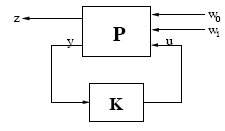
FIGURE 1.2
Feedback Configuration for Nonlinear Mixed ${\mathcal{H}}_2$/${\mathcal{H}}_{\infty }$-Control

Notice however here that the HJIEs (1.29) and DHJIE (1.30) are more involved, in the sense that they are time-varying or evolution PDEs. In the case of (1.29), the solution is a single function of two variables x and t that is also required to satisfy the boundary condition $V\left(x,T\right)=0\forall x\in \mathcal{X};$ while in the case of the DHJIE (1.30), the solution is a set of K + 1 functions with the last function required to also satisfy the boundary conditions $V\left(x,K+1\right)=0\forall x\in \mathcal{X}$. These equations are notoriously difficult to solve and will be the subject of discussion in the last chapter.

1.2.1    Mixed ${\mathcal{H}}_2$/${\mathcal{H}}_{\infty }$-Control Problem

We now consider a different set-up for the ${\mathcal{H}}_{\infty }$-control problem; namely, the problem of mixing two cost functions to achieve disturbance-attenuation and at the same time minimizing the output energy of the system. It is well known that we can only solve the suboptimal ${\mathcal{H}}_{\infty }$-control problem easily, and therefore ${\mathcal{H}}_{\infty }$-controllers are hardly unique. However, ${\mathcal{H}}_2$controllers [92, 292] can be designed optimally. It therefore follows that, by mixing the two criterion functions, one can achieve the benefits of both types of controllers, while at the same time, try to recover some form of uniqueness for the controller. This philosophy led to the formulation of the mixed ${\mathcal{H}}_2$/${\mathcal{H}}_{\infty }$-control problem.

A typical set-up for this problem is shown in Figure 1.2 with $w=\left(\begin{array}{l}{w}_0\\ w_1\end{array}\right)$, where the signal w₀ is a Gaussian white noise signal (or bounded-spectrum signal), while w₁(t) is a bounded-power or energy signal. Thus, the induced norm from the input w₀ to z is the ${\mathcal{L}}_2$-norm (respectively ℓ₂ -norm) of the plant P, i.e.,

$\begin{array}{l}\Vert P^c\Vert {ℒ}_2\triangleq \underset{0\ne w_0\in \mathcal{S}}{\sup }\frac{\Vert z\Vert p}{\Vert w_0\Vert \mathcal{S}},\\ \Vert P^d\Vert l_2\triangleq \underset{0\ne w_0,k\in \mathcal{S}\text{'}}{\sup }\frac{\Vert z\Vert p\text{'}}{\Vert w_0\Vert \mathcal{S}\text{'}},\end{array}$

while the induced norm from w₁ to z is the ${\mathcal{L}}_2$-norm (respectively ℓ_∞-norm) of P, i.e.,

$\begin{array}{l}\Vert P^c\Vert {ℒ}_{\infty }\triangleq \underset{0\ne w_1\in p}{\sup }\frac{{\Vert z\Vert }_2}{{\Vert w_1\Vert }_2},\\ \Vert P^d\Vert l_{\infty }\triangleq \underset{0\ne w_1\in p\text{'}}{\sup }\frac{{\Vert z\Vert }_2}{{\Vert w_1\Vert }_2},\end{array}$

where

$\begin{array}{l}\mathcal{P}\triangleq \left\{w\left(t\right);w\in {ℒ}_{\infty },R_{ww}\left(\tau \right),S_{ww}\left(j\omega \right)\text{exist for all}\tau \text{and all}\omega \text{resp}\text{.,}{\Vert w\Vert }_p^2<\infty \right\},\\ \mathcal{S}\triangleq \left\{w\left(t\right);w\in {ℒ}_{\infty },R_{ww}\left(\tau \right),S_{ww}\left(j\omega \right)\text{exist for all}\tau \text{and all}\omega \text{resp}\text{.,}{\Vert S_{ww}\left(j\omega \right)\Vert }_{\infty }<\infty \right\},\\ \mathcal{P}\text{'}\triangleq \left\{w;w\in l_{\infty },R_{ww}\left(k\right),S_{ww}\left(j\omega \right)\text{exist for all}k\text{and all}\omega \text{resp}\text{.,}{\Vert w\Vert }_{p\text{'}}^2<\infty \right\},\\ \mathcal{S}\text{'}\triangleq \left\{w;w\in l_{\infty },R_{ww}\left(k\right),{\mathcal{S}}_{ww}\left(j\omega \right)\text{exist for all}k\text{and all}\omega \text{resp}\text{.,}{\Vert S_{ww}\left(j\omega \right)\Vert }_{\infty }<\infty \right\},\\ {\Vert z\Vert }_p^2\triangleq \underset{T\to \infty }{\lim }\frac{1}{2T}{\displaystyle \underset{-T}{\overset{T}{\int }}{\Vert z\left(t\right)\Vert }^{2}dt,{\Vert z\Vert }_{p\text{'}}^2\triangleq }\underset{K\to \infty }{\lim }\frac{1}{2K}{\displaystyle \sum _{k=-K}^K{\Vert z_k\Vert }^2,}\\ {\Vert w_0\Vert }_{\mathcal{S}}^2={\Vert S_{w_0{w}_0}\left(j\omega \right)\Vert }_{\infty },{\Vert w_0\Vert }_{\mathcal{S}\text{'}}^2={\Vert S_{w_0{w}_0}\left(j\omega \right)\Vert }_{\infty },\end{array}$

and R_ww(τ), S_ww(jω) (equivalently R_ww(k), S_ww(jω)) are the autocorrelation and power spectral-density matrices [152] of w(t) (equivalently w_k) respectively. Notice also that $\Vert (.)\Vert p$ and ${\Vert (.)\Vert }_{\mathcal{S}}$ are seminorms. In addition, if the plant is stable, we replace the induced ℓ-norms (resp. ℓ-norms) above by their equivalent H-subspace norms.

Since minimizing the ${\mathcal{H}}_{\infty }$-induced norm as defined above, over the set of admissible controllers is a difficult problem (i.e., the optimal ${\mathcal{H}}_{\infty }$-control problem is difficult to solve exactly [92, 101]), whereas minizing the induced ${\mathcal{H}}_2$-norm and obtaining optimal ${\mathcal{H}}_2$- controllers is an easy problem, the objective of the mixed ${\mathcal{H}}_2$/${\mathcal{H}}_{\infty }$ design philosophy is then to minimize ${\Vert P\Vert }_{{ℒ}_2}$ (equivalently ${\Vert P\Vert }_{l_2}$) while rendering ${\Vert P^c\Vert }_{{ℒ}_{\infty }}\le {\text{γ}}^{\star }$ (resp. ${\Vert P^d\Vert }_{l_{\infty }}\le {\text{γ}}^{\star }$ ) for some prescribed number γ^⋆ > 0. Such a problem can be formulated as a two-player nonzero-sum differential game with two cost functionals:

$J_1\left(u,w\right)={\displaystyle \underset{t_0}{\overset{T}{\int }}\left({\text{γ}}^2{\Vert w\left(\tau \right)\Vert }^2-{\Vert z\left(\tau \right)\Vert }^2\right)d\tau }$

(1.31)

$J_2\left(u,w\right)={\displaystyle \underset{t_0}{\overset{T}{\int }}{\Vert z\left(\tau \right)\Vert }^{2}d\tau }$

(1.32)

or equivalently

$J_{1k}\left(u,w\right)={\displaystyle \sum _{k=k_0}^K\left({\text{γ}}^2{\Vert w_k\Vert }^2-{\Vert z_k\Vert }^2\right)}$

(1.33)

$J_{2k}\left(u,w\right)={\displaystyle \sum _{k=K_0}^K{\Vert z_k\Vert }^2}$

(1.34)

for the finite-horizon problem. Here, the first functional is associated with the ${\mathcal{H}}_{\infty }$-constraint criterion, while the second functional is related to the output energy of the system or ${\mathcal{H}}_2$-criterion. Moreover, here we wish to solve an associated mixed ${\mathcal{H}}_2$/${\mathcal{H}}_{\infty }$ problem in which w is comprised of a single disturbance signal $w\in \mathcal{W}\subset {ℒ}_2\left(\left[t_0,\infty \right),{\Re }^r\right)$ (equivalently $w\in \mathcal{W}\subset l_2\left(\left[k_0,\infty \right),{\Re }^r\right)$). It can easily be seen that by making J₁ ≥ 0 (respectively J_1k ≥ 0) then the ${\mathcal{H}}_{\infty }$ constraint ${\Vert P\Vert }_{{ℒ}_{\infty }}\le \text{γ}$ is satisfied. Subsequently, minimizing J₂ (respectively J_2k) will achieve the ${\mathcal{H}}_2$/${\mathcal{H}}_{\infty }$ design objective. Moreover, if we assume also that $\mathcal{U}\subset {ℒ}_2\left(\left[t_0,\infty \right),{\Re }^k\right)$ (equivalently $\mathcal{U}\subset l_2\left(\left[k_0,\infty \right),{\Re }^k\right)$) then under closed-loop perfect information, a Nash-equilibrium solution to the above game is said to exist if we can find a pair of strategies (u^⋆, w^⋆> ) such that

$J_1\left(u^{\star },w^{\star }\right)\le J_1\left(u^{\star },w\right)\forall w\in \mathcal{W}\text{,}$

(1.35)

$J_2\left(u^{\star },w^{\star }\right)\le J_2\left(u,w^{\star }\right)\forall u\in \mathcal{U}\text{.}$

(1.36)

Equivalently for J_1k(u^⋆, w^⋆ ), J_2k(u^⋆ , w^⋆).

Furthermore, by minimizing the first objective with respect to w and substituting in the second objective which is then minimized with respect to u, the pair of Nash-equilibrium strategies can be found. A necessary and sufficient condition for optimality in such a differentail game is provided by a pair of cross-coupled HJIEs (resp. DHJIEs). For the state-feedback problem and the case of the plant P^c given by equation (1.1) or P^d given by (1.2), the governing equations can be obtained by the dynamic-programming principle or the theory of dissipative systems to be

$\begin{array}{l}{Y}_t\left(x,t\right)=-\underset{w\in \mathcal{W}}{\inf }\left\{Y_x\left(x\right)f\left(x,u^{\star }\left(x\right),w\left(x\right)\right)-{\text{γ}}^2{\Vert w\left(x\right)\Vert }^2+{\Vert z^{\star }\left(x\right)\Vert }^2\right\},Y\left(x,T\right)=0,x\in \mathcal{X},\\ x\in \mathcal{X}\text{,}\end{array}$

$\begin{array}{l}{V}_t\left(x,t\right)=-\underset{u\in \mathcal{U}}{\inf }\left\{V_x\left(x\right)f\left(x,u\left(x\right),w^{\star }\left(x\right)\right)+{\Vert z^{\star }\left(x\right)\Vert }^2\right\}=0,V\left(x,T\right)=0,\\ x\in \mathcal{X},\end{array}$

or

$\begin{array}{l}Y\left(x,k\right)=\underset{w_k\in \mathcal{W}}{\min }\left\{Y\left(f_k\left(x,u_k^{\star }\left(x\right),w_k\right))\text{,}k+1\right){\text{+γ}}^2{\Vert w\left(x\right)\Vert }^2-{\Vert z^{\star }\left(x\right)\Vert }^2\right\};\\ Y\left(x,K+1\right)=0,k=1,\mathrm{\dots },K,x\in \mathcal{X},\end{array}$

$\begin{array}{l}V\left(x,k\right)=\underset{u_k\in \mathcal{U}}{\min }\left\{V(f_k\left(x,u_k\left(x\right),w_k^{\star }\left(x\right)\right)+{\Vert z^{\star }\left(x\right)\Vert }^2\right\};\\ V\left(x,K+1\right)=0,k=1,\mathrm{\dots },K,x\in \mathcal{X},\end{array}$

respectively, for some negative-(semi)definite function $V:\mathcal{X}\to \Re$ and positive-(semi)definite function $V:\mathcal{X}\to \Re$.The solution to the above optimization problem will be the subject of discussion in Chapter 11.

1.2.2    Robust ${\mathcal{H}}_{\infty }$-Control Problem

A primary motivation for the development of ${\mathcal{H}}_{\infty }$-synthesis methods is the design of robust controllers to achieve robust performance in the presence of disturbances and/or model uncertainty due to modeling errors or parameter variations. For all the models and the design methods that we have considered so far, we have concentrated on the problem of disturbance-attenuation using either the pure ${\mathcal{H}}_{\infty }$-criterion or the mixed ${\mathcal{H}}_2$/${\mathcal{H}}_{\infty }$-criterion.

Therefore in this section, we briefly overview the second aspect of the theory.

A typical set-up for studying plant uncertainty and the design of robust controllers is shown in Figure 1.3 below. The third block labelled Δ in the diagram represents the model uncertainty. There are also other topologies for representing the uncertainty depending on the nature of the plant [6, 7, 33, 147, 223, 265, 284]; Figure 1.3 is the simplest of such representations. If the uncertainty is significant in the system, such as unmodelled dynamics or perturbation in the model, then the uncertainty can be represented as a dynamic system with input excited by the plant output and output as a disturbance input to the plant, i.e.,

FIGURE 1.3
Feedback Configuration for Robust Nonlinear ${\mathcal{H}}_{\infty }$-Control

${\text{Δ}}^c:\{\begin{array}{l}\dot{\phi }=\vartheta \left(\phi ,u,v\right),\vartheta \left(0,0,0\right)=0,\phi \left(t_0\right)=0\\ e=\varrho \left(\phi ,u,v\right),\varrho \left(0,0,0\right)=0\end{array}$

or

${\text{Δ}}^d:\{\begin{array}{l}{\dot{\phi }}_k={\vartheta }_k\left({\phi }_k,u_k,v_k\right),{\vartheta }_k\left(0,0,0\right)=0,\phi \left(k_0\right)=0\\ e_k={\varrho }_k\left({\phi }_k,u_k,v_k\right),{\varrho }_k\left(0,0,0\right)=0.\end{array}$

The above basic model can be further decomposed (together with the plant) into a coprime factor model as is done in [34, 223, 265].

On the other hand, if the uncertainty is due to parameter variations caused by, for instance, aging or environmental conditions, then it can be represented as a simple norm-bounded uncertainty as in [6, 7, 261, 284]. For the case of the affine system P^ca or P^da, such a model can be represented in the most general way in which the uncertainty or perturbation comes from the system input and output matrices as well as the drift vector-field f as

$P_{\text{Δ}}^{ca}:\{\begin{array}{l}\dot{x}=\left[f\left(x\right)+\text{Δ}f\left(x\right)\right]+g_1\left(x\right)w+\left[g_2\left(x\right)+\text{Δ}{g}_2\left(x\right)\right]u;x\left(0\right)=x_0\\ z=h_1\left(x\right)+k_{12}\left(x\right)u\\ y=\left[h_2\left(x\right)+\text{Δ}{h}_2\left(x\right)\right]+k_{21}\left(x\right)w\end{array}$

or

$P_{\text{Δ}}^{da}:\{\begin{array}{l}{x}_{k+1}=\left[f\left(x_k\right)+\text{Δ}f\left(x_k\right)\right]+g_1\left(x_k\right)w_k+\left[g_2\left(x_k\right)+\text{Δ}{g}_2\left(x_k\right)\right]u_k;x\left(0\right)=x_0\\ z_k=h_1\left(x_k\right)+k_{12}\left(x_k\right)u_k\\ y_k=\left[h_2\left(x_k\right)+\text{Δ}{h}_2\left(x_k\right)\right]+k_{21}\left(x_k\right)w_k,k\in \mathbf{Z}\end{array}$

respectively, where Δf, Δg₂, Δh₂ belong to some suitable admissible sets.

Whichever type of representation is chosen for the plant, the problem of robustly designing an ${\mathcal{H}}_{\infty }$ controller or mixed ${\mathcal{H}}_2$/${\mathcal{H}}_{\infty }$-controller for the plant $P_{\text{Δ}}^{ca}$ (respectively $P_{\text{Δ}}^{da}$) can be pursued along similar lines as in the case of the nominal model P^ca (respectively P^da) using either state-feedback or output-feedback with some additional complexity due to the presence of the uncertainty. This problem will be discussed for the continuous-time state-feedback case in Chapter 5 and for the the measurement-feedback case in Chapter 6.

1.2.3    Nonlinear ${\mathcal{H}}_{\infty }$-Filtering

Often than not, the states of a dynamic system are not accessible from its output. Therefore, it is necessary to design a scheme for estimating them for the purpose of feedback or other use. Such a scheme involves another dynamic system called an “observer” or “filter.” It is essentially a carbon-copy of the original system which is error-driven. It takes in the past and present output measurements y(t) of the system for a given time span [t₀, t] ⊂ ℜ and generates an estimate of the desired output z which can be the states or some suitable function of them. It is therefore required to be “causal” so that it is implementable.

FIGURE 1.4
Configuration for Nonlinear ${\mathcal{H}}_{\infty }$-Filtering

A typical set-up for filtering is shown in Figure 1.4. The filter is denoted by F and is designed to minimize the worst-case gain from w to the error difference between the actual desired output of the system z and the estimated output $\widehat{z}$; typically z = x in such applications. We can represent the plant P by an affine state-space model with the subscript “f” added to denote a filtering model:

$P_f^{ca}:\{\begin{array}{l}\dot{x}=f\left(x\right)+g_1\left(x\right)w+g_2\left(x\right)w;x\left(t_0\right)=x_0\\ z=h_1\left(x\right)\\ y=h_2\left(x\right)+k_{21}\left(x\right)w\end{array}$

(1.37)

or equivalently

$P_f^{da}:\{\begin{array}{l}{x}_{k+1}=f\left(x_k\right)+g_1\left(x_k\right)w_{};x_{k_0}=x^0\\ z_k=h_1\left(x_k\right)\\ y_k=h_2\left(x_k\right)+k_{21}\left(x_k\right)w_k,k\in \mathbf{Z}\end{array}$

(1.38)

where all the variables and functions have their previous meanings and definitions, and $w\in {ℒ}_2\left[t_0,\infty \right)$ (or equivalently $w\in l_2\left[k_0,\infty \right)$) is a noise signal that is assumed to corrupt the outputs y and z (respectively y_k and z_k) of the system. Then the objective is to design the filter such that

$\underset{w\in {ℒ}_2\left(t_0,\infty \right)}{sup}\frac{{\Vert z-\widehat{z}\Vert }_2^2}{{\Vert w\Vert }_2^2}\le {\text{γ}}^{\star }$

or equivalently

$\underset{w\in l_2\left(t_0,\infty \right)}{sup}\frac{{\Vert z_k-{\widehat{z}}_k\Vert }_2^2}{{\Vert w_k\Vert }_2^2}\le {\text{γ}}^{\star }$

for some prescribed number γ^⋆ > 0 is achieved. If the filter F is configured so that it has identical dynamics as the system, then it can be shown that the solution to the filtering problem is characterized by a (D)HJIE that is dual to that of the state-feedback problem.

1.2.4    Organization of the Book

The book contains thirteen chapters and two appendices. It is loosely organized in two parts: Part I, comprising Chapters 1-4 covers mainly introductory and background material, while Part II comprising Chapters 5-13 covers the real subject matter of the book, dealing with all the various types and aspects of nonlinear ${\mathcal{H}}_{\infty }$-control problems.

Chapter 1 is an introductory chapter. It covers historical perspectives and gives highlights of the contents of the book. Preliminary definitions and notations are also given to prepare the reader for what is to come. In addition, some introduction on differentiable manifolds, mainly definitions, and Lyapunov-stability theory is also included in the chapter to make the book self-contained.

Chapter 2 gives background material on the basics of differential games. It discusses discrete-time and continuous-time nonzero-sum and zero-sum games from which all of the problems in nonlinear ${\mathcal{H}}_{\infty }$-theory are derived and solved. Linear-quadratic (LQ) and two-person games are included as special cases and to serve as examples. No proofs are given for most of the results in this chapter as they are standard, and can be found in wellknown standard references on the subject.

Chapter 3 is devoted to the theory of dissipative systems which is also at the core of the subject of the book. The material presented, however, is well beyond the amount required for elucidating the content matter. The reason being that this theory is not very well known by the control community, yet it pervades almost all the problems of modern control theory, from the LQ-theory and the positive-real lemma, to the ${\mathcal{H}}_{\infty }$-theory and the bounded-real lemma. As such, we have given a complete literature review on this subject and endeavored to include all relevant applications of this theory. A wealth of references is also included for further study.

Chapter 4 is also at the core of the book, and traces the origin of Hamilton-Jacobi theory and Hamiltonian systems to Lagrangian mechanics. The equivalence of Hamiltonian and Lagrangian mechanics is stressed, and the motivation behind the Hamiltonian approach is emphasized. The Hamilton-Jacobi equation is derived from variational principles and the duality between it and Hamilton’s canonical equations is pointed. In this regard, the method of characteristics for first-order partial-differential equations is also discussed in the chapter, and it is shown that Hamilton’s canonical equations are nothing but the characteristic equations for the HJE.

The concept of viscosity and non-smooth solutions of the HJE where smooth solutions and/or Hamiltonians do not exist is also introduced, and lastly the Toda lattice which is a particularly integrable Hamiltonian system, is discussed as an example.

Chapter 5 starts the discussion of nonlinear ${\mathcal{H}}_{\infty }$-theory with the state-feedback problem for continuous-time affine nonlinear time-invariant systems. The solution to this problem is derived from the differential game as well as dissipative systems perspective. The parametrization of a class of full-information controllers is given, and the robust control problem in the presence of unmodelled and parametric uncertainty is also discussed. The approach is then extended to time-varying and delay systems, as well as a more general class of nonlinear systems that are not necessarily affine. In addition, the ${\mathcal{H}}_{\infty }$ almost disturbance-decoupling problem for affine systems is also discussed.

Chapter 6 continues with the discussion in the previous chapter with the output-feedback problem for affine nonlinear systems. First the output measurement-feedback problem is considered and sufficient conditions for the solvability of this problem are given in terms of two uncoupled HJIEs with an additional side-condition. Moreover, it is shown that the controller that solves this problem is observer-based. A parametrization of all output-feedback controllers is given, and the results are also extended to a more general class of nonlinear systems. The robust measurement-feedback problem in the presence of uncertainties is also considered. Finally, the static output-feedback problem is considered, and sufficient conditions for its solvability are also presented in terms of a HJIE together with some algebraic conditions.

In Chapter 7 the discrete-time nonlinear ${\mathcal{H}}_{\infty }$-control problem is discussed. Solution for the full-information, state-feedback and output measurement-feedback problems are given, as well as parametrizations of classes of full-information state and output-feedback controllers. The extension of the solution to more general affine discrete-time systems is also presented. In addition, an approximate and explicit approach to the solution to the problem is also presented.

In Chapter 8 the nonlinear ${\mathcal{H}}_{\infty }$-filtering problem is discussed. Solutions for both the continuous-time and the discrete-time problems are given in terms of dual HJIEs and a coupling condition. Some simulation results are also given to show the performance of the nonlinear ${\mathcal{H}}_{\infty }$-filter compared to the extended Kalman-filter. The robust filtering problem is also discussed.

Chapter 9 discusses the generalization of the ${\mathcal{H}}_{\infty }$-control problems to include singular or ill-posed problems, as well as the ${\mathcal{H}}_{\infty }$-control of singularly-perturbed nonlinear systems with small singular parameters. Both the singular state and measurement-feedback problems are discussed, and the case of cascaded systems is also addressed. However, only the continuous-time results are presented. Furhermore, the state-feedback control problem for nonlinear singularly perturbed continuous-time systems is presented, and a class of composite controllers is also discussed. In addition, Chapter 10 continues with the discussion on singularly perturbed systems and presents a solution to the ${\mathcal{H}}_{\infty }$ infinite-horizon filtering problem for affine nonlinear singularly perturbed systems. Three types of filters, namely, decomposition, aggregate and reduced-order filters are presented, and again sufficient conditions for the solvability of the problem with each filter are presented.

Chapers 11 and 12 are devoted to the mixed ${\mathcal{H}}_2$/${\mathcal{H}}_{\infty }$ nonlinear control and filtering problems respectively. Only the state-feedback control problem is discussed in Chapter 11 and this is complemented by the filtering problem in Chapter 12. The output measurement-feedback problem is not discussed because of its complexity. Moreover, the treatment is exhaustive, and both the continuous and discrete-time results are presented.

Lastly, the book culminates in Chapter 13 with a discussion of some computational approaches for solving Hamilton-Jacobi equations which are the cornerstones of the theory. Iterative as well as exact methods are discussed. But the topic is still evolving, and it is hoped that the chapter will be substantially improved in the future.