5

State-Feedback Nonlinear ${\mathcal{H}}_{\infty }$-Control for Continuous-Time Systems

In this chapter, we discuss the nonlinear ${\mathcal{H}}_{\infty }$ sub-optimal control problem for continuous-time affine nonlinear systems using state-feedback. This problem arises when the states of the system are available, or can be measured directly and used for feedback. We derive sufficient conditions for the solvability of the problem, and we discuss the results for both time-invariant (or autonomous) systems and time-varying (or nonautonomous) systems, as well as systems with a delay in the state. We also give a parametrization of all full-information stabilizing controllers for each system. Moreover, understanding the state-feedback problem will facilitate the understanding of the dynamic measurement-feedback problem which is discussed in the subsequent chapter.

The problem of robust control in the presence of modelling errors and/or parameter variations is also discussed. Sufficient conditions for the solvability of this problem are given, and a class of controllers is presented.

5.1    State-Feedback ${\mathcal{H}}_{\infty }$-Control for Affine Nonlinear Systems

The set-up for this configuration is shown in Figure 5.1, where the plant is represented by an affine causal state-space system defined on a smooth n-dimensional manifold χ ⊆ ℜⁿ in local coordinates x = (x₁,…, x_n):

${\mathrm{\Sigma }}^a:\{\begin{array}{l}\dot{x}=f\left(x\right)+g_1\left(x\right)w+g_2\left(x\right)u;x\left(t_0\right)=x_0\\ y=x\\ z=h_1\left(x\right)+k_{12}\left(x\right)u\end{array}$

(5.1)

where x ∈ $\mathcal{X}$ is the state vector, u ∈ $\mathcal{U}$ ⊆ ℜ^p is the p-dimensional control input, which belongs to the set of admissible controls $\mathcal{U},w\in \mathcal{W}$ is the disturbance signal, which belongs to the set $\mathcal{W}\subset {ℒ}_2\left([t_0,\infty ),{\Re }^r\right)$ of admissible disturbances, the output y ∈ ℜⁿ is the states-vector of the system which is measured directly, and z ∈ ℜ^s is the output to be controlled. The functions $f:\mathcal{X}\to V^{\infty }\left(\mathcal{X}\right),g_1:\mathcal{X}\to {ℳ}^{n\times r}\left(\mathcal{X}\right),g_2:\mathcal{X}\to {ℳ}^{n\times p}\left(\mathcal{X}\right),h_1:\mathcal{X}\to {\Re }^s,\text{and}{k}_{12}:\mathcal{X}\to {ℳ}^{p\times m}\left(\mathcal{X}\right)$ are assumed to be real C^∞-functions of x. Furthermore, we assume without loss of generality that x = 0 is a unique equilibrium point of the system with u = 0, w = 0, and is such that f(0) = 0, h₁(0) = 0. We also assume that the system is well defined, i.e., for any initial state x(t₀) ∈ $\mathcal{X}$ and any admissible input u(t) ∈ $\mathcal{U}$, there exists a unique solution x(t, t₀, x₀, u) to (5.1) on [t₀, ∞) which continuously depends on the initial conditions, or the system satisfies the local existence and uniqueness theorem for ordinary differential-equations [157].

Again Figure 5.1 also shows that for this configuration, the states of the plant are accessible and can be directly measured for the purpose of feedback control. We begin with the definition of smooth-stabilizability and also recall the definition of ${ℒ}_2$-gain of the system Σ^a.

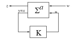
FIGURE 5.1
Feedback Configuration for State-Feedback Nonlinear ${\mathcal{H}}_{\infty }$ -Control

Definition 5.1.1 (Smooth-stabilizability). The nonlinear system Σ^a (or simply [f, g₂]) is locally smoothly-stabilizable if there exists a C⁰-function F : $\mathcal{U}$ ⊂ $\mathcal{X}$ → ℜ^p, F (0) = 0, such that $\dot{x}$ = f(x)+g₂(x)F (x) is locally asymptotically stable. The system is smoothly-stabilizable if U = $\mathcal{X}$.

Definition 5.1.2 The nonlinear system Σ^a is said to have locally ${ℒ}_2$-gain from w to z in U ⊂ $\mathcal{X}$, less than or equal to γ, if for any x₀ ∈ $\mathcal{U}$ and fixed u, the response z of the system corresponding to any w ∈ $\mathcal{W}$ satisfies:

${\int }_{t_0}^T{\Vert z\left(t\right)\Vert }^{2}dt\le {\gamma }^2{\displaystyle {\int }_{t_0}^T{\Vert w\left(t\right)\Vert }^{2}dt+\beta \left(x_0\right),}\forall T>t_0,$

for some bounded C⁰ function β : U → ℜ such that β(0) = 0. The system has ${ℒ}_2$-gain ≤ γ if the above inequality is satisfied for all x ∈ $\mathcal{X}$, or U =$\mathcal{X}$.

Since we are interested in designing smooth feedback laws for the system to make it asymptotically or internally stable, the requirement of smooth-stabilizability for the system will obviously be necessary for the solvability of the problem before anything else. The suboptimal state-feedback nonlinear ${\mathcal{H}}_{\infty }$-control or local disturbance-attenuation problem with internal stability, can then be formally defined as follows.

Definition 5.1.3 (State-Feedback Nonlinear ${\mathcal{H}}_{\infty }$ (Suboptimal)-Control Problem (SFBNLHICP)). The state-feedback ℌ_∞ suboptimal control or local disturbance-attenuation problem with internal stability for the system Σ^a, is to find a static state-feedback control function of the form

$u=\alpha \left(x,t\right),\alpha :{\Re }_{+}\times N\to {\Re }^P,N\subset \mathcal{X}$

(5.2)

for some smooth function α depending on x and possibly t only, such that the closed-loop system:

${\sum }_{clp}^a:\{\begin{array}{l}\dot{x}=f\left(x\right)+g_1\left(x\right)w+g_2\left(x\right)\alpha \left(x,t\right);x\left(t_0\right)=x_0\\ z=h_1\left(x\right)+k_{12}\left(x\right)\alpha \left(x,t\right)\end{array}$

(5.3)

has, for all initial conditions x(t₀) ∈ N, locally ${ℒ}_2$-gain from the disturbance signal w to the output z less than or equal to some prescribed number γ^$\star$ > 0 with internal stability, or equivalently, the closed-loop system achieves local disturbance-attenuation less than or equal to γ^$\star$ with internal stability.

Internal stability of the system in the above definition means that all internal signals in the system, or trajectories, are bounded, which is also equivalent to local asymptotic-stability of the closed-loop system with w = 0 in this case.

Remark 5.1.1 The optimal problem in the above definition is to find the minimum γ^$\star$ > 0 for which the ${ℒ}_2$-gain is minimized. This problem is however more difficult to solve.

One way to measure the ${ℒ}_2$-gain (or with an abuse of the terminology, ${\mathcal{H}}_{\infty }$-norm) of the system (5.1), is to excite it with a periodic input w_T ∈ W, where W ⊂ $\mathcal{W}$ is the subspace of periodic continuous-time functions (e.g., a sinusoidal signal), and to measure the steady-state output response z_ss(.) corresponding to the steady-state state response x_ss(.). Then the ${ℒ}_2$-gain can be calculated as

$\Vert {\mathrm{\Sigma }}^a\Vert {\mathcal{H}}_{\infty }=\underset{w\in W}{\sup }\frac{\Vert z_{ss}\Vert T}{\Vert w\Vert T}$

where

$\Vert w\Vert T=\frac{1}{T}{\left({\displaystyle {\int }_{t_0}^{t_0+T}{\Vert w\left(s\right)\Vert }^{2}ds}\right)}^{\frac{1}{2}},\Vert z_{ss}\Vert T=\frac{1}{T}{\left({\displaystyle {\int }_{t_0}^{t_0+T}{\Vert w\left(s\right)\Vert }^{2}ds}\right)}^{\frac{1}{2}}.$

Returning now to the SFBNLHICP, to derive sufficient conditions for the solvability of this problem, we apply the theory of differential games developed in Chapter 2. It is fairly clear that the problem of choosing a control function u^$\star$(.) such that the ${ℒ}_2$-gain of the closed-loop system from w to z is less than or equal to γ > 0, can be formulated as a two-player zero-sum differential game with u the minimizing player’s decision, w the maximizing player’s decision, and the objective functional:

$\underset{u\in \mathcal{U}}{\min }\underset{w\in \mathcal{W}}{\max }J\left(u,w\right)=\frac{1}{2}{\displaystyle {\int }_{t_0}^T\left[{\Vert z\left(t\right)\Vert }^2-{\gamma }^2{\Vert w\left(t\right)\Vert }^2\right]dt,}$

(5.4)

subject to the dynamical equations (5.1) over a finite time-horizon T > t₀.

At this point, we separate the problem into two subproblems; namely, (i) achieving local disturbance-attenuation and (ii) achieving local asymptotic-stability. To solve the first problem, we allow w to vary over all possible disturbances including the worst-case disturbance, and search for a feedback control function $u:\mathcal{X}\times \Re \to \mathcal{U}$ depending on the current state information, that minimizes the objective functional J(., .) and renders it nonpositive for all w starting from x₀ = 0. By so doing, we have the following result.

Proposition 5.1.1 Suppose for γ = γ^$\star$ there exists a locally defined feedback-control function u^$\star$ : N × ℜ → ℜ^p, 0 ∈ N ⊂ $\mathcal{X}$, which is possibly time-varying, and renders J(., .) nonpositive for the worst possible disturbance w^$\star$ ∈ $\mathcal{W}$ (and hence for all w ∈ $\mathcal{W}$) for all T > 0. Then the closed-loop system has locally ${ℒ}_2$-gain ≤ γ^$\star$.

Proof:

$J\left(u^{\star },w^{\star }\right)\le 0\Rightarrow \Vert z\Vert {\mathcal{L}}_2\left[t_0,T\right]\le {\gamma }^{\star }\Vert w\Vert {\mathcal{L}}_2\left[t_0,T\right]\forall T>0.\square$

To derive the sufficient conditions for the solvability of the first sub-problem, we define the value-function for the game V : $\mathcal{X}$ × [0, T ] → ℜ as

$V\left(t,x\right)=\underset{u}{\inf }\underset{w}{\sup }\frac{1}{2}{\displaystyle {\int }_t^T\left[{\Vert z\left(\tau \right)\Vert }^2-\gamma {\Vert w\left(\tau \right)\Vert }^2\right]d\tau }$

and apply Theorem 2.4.2 from Chapter 2. Consequently, we have the following theorem.

Theorem 5.1.1 Consider the SFBNLHICP problem as a two-player zero-sum differential game with the cost functional (5.4). A pair of strategies (u^$\star$ (x, t), w^$\star$ (x, t)) provides, under feedback information structure, a saddle-point solution to the game such that

$J\left(u^{\star },w\right)\le J\left(u^{\star },w^{\star }\right)\le J\left(u,w^{\star }\right),$

if the value-function V is C¹ and satisfies the HJI-PDE (HJIE):

$\begin{array}{l}-V_t\left(x,t\right)=\underset{u}{\min }\underset{w}{\sup }\left\{V_x\left(x,t\right)\left[f\left(x\right)+g1\left(x\right)w+g2\left(x\right)u\right]+\frac{1}{2}\left({\Vert z\Vert }^2-{\gamma }^2{\Vert w\Vert }^2\right)\right\}\\ =\underset{w}{\sup }\underset{u}{\min }\left\{V_x\left(x,t\right)\left[f\left(x\right)+g1\left(x\right)w+g2\left(x\right)u\right]+\frac{1}{2}\left({\Vert z\Vert }^2-\frac{1}{2}{\gamma }^2{\Vert w\Vert }^2\right)\right\}\\ =V_x\left(x,t\right)\left[f\left(x\right)+g1\left(x\right)w^{\star }\left(x,t\right)+g2\left(x\right)u^{\star }\left(x,t\right)\right]+\frac{1}{2}{\Vert h_1\left(x\right)+k_{12}\left(x\right)u^{\star }\left(x,t\right)\Vert }^2-\\ \frac{1}{2}{\gamma }^2{\Vert w^{\star }\left(x,t\right)\Vert }^2;V\left(x,T\right)=0.\end{array}$

(5.5)

Next, to find the pair of feedback strategy (u^$\star$, w^$\star$ ) that satisfies Isaac’s equation (5.5), we form the Hamiltonian function $H:T^{\star }\mathcal{X}\times \mathcal{U}\times \mathcal{W}\to \Re$ for the problem:

$H\left(x,p,u,w\right)=p^T\left(f\left(x\right)+g_1\left(x\right)w+g_2\left(x\right)u\right)+\frac{1}{2}{\Vert h_1\left(x\right)+k_{12}\left(x\right)u\Vert }^2-\frac{1}{2}{\gamma }^2{\Vert w\Vert }^2,$

(5.6)

and search for a unique saddle-point (u^$\star$, w^$\star$ ) such that

$H\left(x,p,u^{\star },w\right)\le H\left(x,p,u^{\star },w^{\star }\right)\le H\left(x,p,u,w^{\star }\right)$

(5.7)

for each (u, w) and each (x, p), where p is the adjoint variable.

Since the function H(., ., ., .) is C² in both u and w, the above problem can be solved by applying the necessary conditions for an unconstrained optimization problem. However, the only problem that might arise is if the coefficient matrix of u is singular. This more general problem will be discussed in Chapter 9. But in the meantime to overcome this problem, we need the following assumption.

Assumption 5.1.1 The matrix

$R\left(x\right)=k_{12}^T\left(x\right)k_{12}\left(x\right)$

is nonsingular for all x ∈ $\mathcal{X}$.

Under the above assumption, the necessary conditions for optimality for u and w provided by the minimum (maximum) principle [175] are

$\frac{\partial H}{\partial u}\left(u^{\star },w\right)=0,\frac{\partial H}{\partial w}\left(u,w^{\star }\right)=0$

for all (u, w). Application of these conditions gives

$u^{\star }\left(x,p\right)=-R^{-1}\left(x\right)\left(g_2^T\left(x\right)p+k_{12}^T\left(x\right)h_1\left(x\right)\right),$

(5.8)

$w^{\star }\left(x,p\right)=\frac{1}{{\gamma }^2}{g}_1^T\left(x\right)p.$

(5.9)

Moreover, since by assumption R(.) is nonsingular and therefore positive-definite, and γ > 0, the above equilibrium-point is clearly an optimizer of J(u, w). Further, we can write

$H\left(x,p,u,w\right)=H^{\star }\left(x,p\right)+\frac{1}{2}{\Vert u-u^{\star }\Vert }_{R\left(x\right)}^2-\frac{1}{2}{\gamma }^2{\Vert w-w^{\star }\Vert }^2,$

(5.10)

where

$H^{\star }\left(x,p\right)=H\left(x,p,u^{\star }\left(x,p\right),w^{\star }\left(x,p\right)\right)$

and the notation ‖a‖ _Q stands for a^TQa for any a ∈ ℜⁿ, Q ∈ ℜ^n×n. Substituting u^$\star$ and w^$\star$ in turns in (5.10) show that the saddle-point conditions (5.7) are satisfied.

Now assume that there exists a C¹ positive-semidefinite solution V : $\mathcal{X}$ → ℜ to Isaac’s equation (5.5) which is defined in a neighborhood N of the origin, that vanishes at x = 0 and is time-invariant (this assumption is plausible since H(., ., ., .) is time-invariant). Then the feedbacks (u^$\star$, w^$\star$) necessarily exist, and choosing

$p=V_x^T\left(x\right)$

in (5.10) yields the identity:

$\begin{array}{l}H\left(x,V_x^T\left(x\right),w,u\right)=V_x\left(x\right)\left(f\left(x\right)+g_1\left(x\right)w+g_2\left(x\right)u\right)+\frac{1}{2}{\Vert h_1\left(x\right)+k_{12}\left(x\right)u\Vert }^2-\frac{1}{2}{\gamma }^2{\Vert w\Vert }^2\\ =H^{\star }\left(x,V_x^T\left(x\right)\right)+\frac{1}{2}{\Vert u-u^{\star }\Vert }_{R\left(x\right)}^2+\frac{1}{2}{\gamma }^2{\Vert w-w^{\star }\Vert }^2.\end{array}$

Finally, notice that for u = u^$\star$ and w = w^$\star$, the above identity yields

$H\left(x,V_x^T\left(x\right),w^{\star },u^{\star }\right)=H^{\star }\left(x,V_x^T\left(x\right)\right)$

which is exactly the right-hand-side of (5.5), and for this equation to be satisfied, V(.) must be such that

$H^{\star }\left(x,V_x^T\left(x\right)\right)=0$

(5.11)

The above condition (5.11) is the time-invariant HJIE for the disturbance-attenuation problem. Integration of (5.11) along the trajectories of the closed-loop system with $\alpha \left(x\right)=u^{\star }\left(x,V_x^T\left(x\right)\right)$ (independent of t!) starting from t = t₀ and x(t₀) = x₀, to t = T > t₀ and x(T ) yields

$V\left(x\left(T\right)\right)-V\left(x_0\right)\le \frac{1}{2}{\displaystyle {\int }_{t_0}^T\left({\gamma }^2{\Vert w\Vert }^2-{\Vert z\Vert }^2\right)dt}\ge 0\forall w\in \mathcal{W}.$

This means J(u^$\star$, w) is nonpositive for all w ∈ $\mathcal{W}$, and consequently implies the ${ℒ}_2$-gain of the system is less than or equal to γ. This also solves part (i) of the state-feedback suboptimal ${\mathcal{H}}_{\infty }$-control problem. Before we consider part (ii) of the problem, we make the following simplifying assumption.

Assumption 5.1.2 The output vector h₁(.) and weighting matrix k₁₂(.) are such that

$k_{12}^T\left(x\right)k_{12}\left(x\right)=I$

and

$h_1^T\left(x\right)k_{12}\left(x\right)=0$

for all x ∈ $\mathcal{X}$. Equivalently, we shall henceforth write $z=\left[\begin{array}{c}{h}_1\left(x\right)\\ u\end{array}\right]$ under this assumption.

Remark 5.1.2 The above assumption implies that there are no cross-product terms in the performance or cost-functional (5.4), and the weighting on the control is unity.

Under the above assumption 5.1.2, the HJIE (5.11) becomes

$V_{\left(x\right)}\left(x\right)f\left(x\right)+\frac{1}{2}{V}_{\left(x\right)}\left(x\right)\left[\frac{1}{{\gamma }^2}{g}_1\left(x\right)g_1^T\left(x\right)-g_2\left(x\right)g_1^T\left(x\right)\right]V_x^T\left(x\right)+\frac{1}{2}{h}_1^T\left(x\right)h_1\left(x\right)=0,V\left(0\right)=0,$

(5.12)

and the feedbacks (5.8), (5.9) become

$u^{\star }\left(x\right)=-g_2^T\left(x\right)V_x^T\left(x\right)$

(5.13)

$w^{\star }\left(x\right)=\frac{1}{{\gamma }^2}{g}_1^T\left(x\right)V_x^T\left(x\right).$

(5.14)

Thus, the above condition (5.12) together with the associated feedbacks (5.13), (5.14) provide a sufficient condition for the solvability of the state-feedback suboptimal ${\mathcal{H}}_{\infty }$ problem on the infinite-time horizon when T → ∞.

On the other hand, let us consider the finite-horizon problem as defined by the cost functional (5.4) with T < ∞. Assuming there exists a time-varying positive-semidefinite C¹ solution V : $\mathcal{X}$ × ℜ → ℜ to the HJIE (5.5) such that

$p=V_x^T\left(x,t\right),$

then substituting in (5.8), (5.9) and the HJIE (5.5) under the Assumption 5.1.2, we have

$u^{\star }\left(x,t\right)=-g_2^T\left(x\right)V_x^T\left(x,t\right)$

(5.15)

$w^{\star }\left(x,t\right)=\frac{1}{{\gamma }^2}{g}_1^T\left(x\right)V_x^T\left(x,t\right),$

(5.16)

where V satisfies the HJIE

$\begin{array}{l}{V}_t\left(x,t\right)+V_x\left(x,t\right)f\left(x\right)+\frac{1}{2}{V}_x\left(x,t\right)\left[\frac{1}{{\gamma }^2}{g}_1\left(x\right)g_1^T\left(x\right)-g_2\left(x\right)g_2^T\left(x\right)\right]V_x^T\left(x,t\right)+\\ \frac{1}{2}{h}^T\left(x\right)h_1\left(x\right)=0,V\left(x,T\right)=0.\end{array}$

(5.17)

Therefore, the above HJIE (5.17) gives a sufficient condition for the solvability of the finite-horizon suboptimal ${\mathcal{H}}_{\infty }$ control problem and the associated feedbacks.

Let us consider an example at this point.

Example 5.1.1 Consider the nonlinear system with the associated penalty function

$\begin{array}{l}{\dot{x}}_1=x_2\\ {\dot{x}}_2=-x_1-\frac{1}{2}{x}_2^3+x_{2}w+u\\ z=\left[\begin{array}{l}{x}_2\\ u\end{array}\right].\end{array}$

The HJIE (5.12) corresponding to this system and penalty function is given by

$x_2{V}_{x_1}-x_1{V}_{x_2}-\frac{1}{2}{x}_2^3{V}_{x_2}+\frac{1}{2}\frac{x_2^2\left(x_2^2-{\gamma }^2\right)}{{\gamma }^2}+\frac{1}{2}{x}_2^2=0.$

Let γ = 1 and choose

$V_{x_1}=x_1,V_{x_2}=x_2.$

Then we see that the HJIE is solved with $V\left(x\right)=\frac{1}{2}\left(x_1^2+x_2^2\right)$ which is positive-definite. The associated feedbacks are given by

$u^{\star }=-x_2,w^{\star }=x_2^2.$

It is also interesting to notice that the above solution V to the HJIE (5.12) is also a Lyapunov-function candidate for the free system: ${\dot{x}}_1=x_2,{\dot{x}}_2=-x_1-\frac{1}{2}{x}_2^3.$

Next, we consider the problem of asymptotic-stability for the closed-loop system (5.3), which is part (ii) of the problem. For this, let

$\alpha \left(x\right)=u^{\star }\left(x\right)=-g_2^T\left(x\right)V_x^T\left(x\right),$

where V(.) is a smooth positive-semidefinite solution of the HJIE (5.12). Then differentiating V along the trajectories of the closed-loop system with w = 0 and using (5.12), we get

$\begin{array}{l}\dot{V}\left(x\right)=V_x\left(x\right)\left(f\left(x\right)-g_2\left(x\right)g_2^T\left(x\right)V_x\left(x\right)\right)\\ =-\frac{1}{2}\Vert u^{\star }\Vert {}^2-\frac{1}{2}{\gamma }^2{\Vert w^{\star }\Vert }^2-\frac{1}{2}{h}^T\left(x\right)h_1\left(x\right)\le 0,\end{array}$

where use has been made of the HJIE (5.12). Therefore, $\dot{V}$ is nonincreasing along trajectories of the closed-loop system, and hence the system is stable in the sense of Lyapunov. To prove local asymptotic-stability however, an additional assumption on the system will be necessary.

Definition 5.1.4 The nonlinear system Σ^a is said to be locally zero-state detectable if there exists a neighborhood U ⊂$\mathcal{X}$ of x = 0 such that, for all x(t₀) ∈ $\mathcal{U}$, if z(t) ≡ 0, u(t) ≡ 0 for all t ≥ t₀, it implies that ${\lim }_{t\to \infty }x\left(t,t_0,x_0,u\right)=0$. It is zero-state detectable if U = $\mathcal{X}$.

Thus, if we assume the system Σ^a to be locally zero-state detectable, then it is seen that for any trajectory of the system x(t) ∈ $\mathcal{U}$ such that $\dot{V}\left(x(t)\right)\equiv 0$ for all t ≥ t_s for some t_s ≥ t₀, it is necessary that u(t) ≡ 0 and z(t) ≡ 0 for all t ≥ t_s. This by zero-state detectability implies that ${\lim }_{t\to \infty }x\left(t\right)=0.$ Finally, since x = 0 is the only equilibrium-point of the system in $\mathcal{U}$, by LaSalle’s invariance-principle, we can conclude local asymptotic-stability.

The above result is summarized as the solution to the state-feedback ${\mathcal{H}}_{\infty }$ sub-optimal control problem (SFBNLHICP) in the next theorem after the following definition.

Definition 5.1.5 A nonnegative function V : $\mathcal{X}$ → ℜ is proper if the level set V⁻¹([0, a]) = {x ∈ $\mathcal{X}$|0 ≤ V (x) ≤ a} is compact for each a > 0.

Theorem 5.1.2 Consider the nonlinear system Σ^a and the SFBNLHICP for the system. Assume the system is smoothly-stabilizable and locally zero-state detectable in N ⊂ $\mathcal{X}$. Suppose also there exists a smooth positive-semidefinite solution to the HJIE (5.12) in N. Then the control law

$u^{\star }=\alpha \left(x\right)=-g_2^T\left(x\right)V_x^T\left(x\right),x\in N$

(5.18)

solves the SFBNLHICP locally in N. If in addition Σ^a is globally zero-state detectable and V is proper, then u^$\star$ solves the problem globally.

Proof: The first part of the theorem has already been proven in the above developments. For the second part regarding global asymptotic-stability, note that, if V is proper, then V is a global solution of the HJIE (5.11), and the result follows by application of LaSalle’s invariance-principle from Chapter 1 (see also the References [157, 268]). □

The existence of a C² solution to the HJIE (5.12) is related to the existence of an invariant-manifold for the corresponding Hamiltonian system:

$X_{H_{\gamma }^{\star }}:\{\begin{array}{l}\frac{dx}{dt}=\frac{\partial H_{\gamma }^{\star }\left(x,p\right)}{\partial p}\\ \frac{dp}{dt}=-\frac{\partial H_{\gamma }^{\star }\left(x,p\right)}{\partial x},\end{array}$

(5.19)

where

$H_{\gamma }^{\star }\left(x,p\right)=p^{T}f\left(x\right)+\frac{1}{2}{p}^T\left[\frac{1}{{\gamma }^2}{g}_1\left(x\right)g_1^T\left(x\right)-g_2\left(x\right)g_2^T\left(x\right)\right]P+\frac{1}{2}{h}_1^T\left(x\right)h_1\left(x\right).$

It can be seen then that, if V is a C² solution of the Isaacs equation, then differentiating H^$\star$ (x, p) in (5.11) with respect to x we get

${\left(\frac{\partial H_{\gamma }^{\star }}{\partial x}\right)}_{p=V_x^T}+{\left(\frac{\partial H_{\gamma }^{\star }}{\partial p}\right)}_{p=V_x^T}\frac{\partial V_x^T}{\partial x}=0,$

and since the Hessian matrix

$\frac{\partial V_x^T}{\partial x}$

is symmetric, it implies that the submanifold

$\text{M=}\left\{\left(x,p\right):p=V_x^T\left(x\right)\right\}$

(5.20)

is invariant under the flow of the Hamiltonian vector-field $X_{H_{\gamma }^{\star }}$, i.e.,

${\left(\frac{\partial H_{\gamma }^{\star }}{\partial x}\right)}_{p=V_x^T}=-{\left(\frac{\partial H_{\gamma }^{\star }}{\partial p}\right)}_{p=V_x^T}\frac{\partial V_x^T}{\partial x}.$

The above developments have considered the SFBNLHICP from a differential games perspective. In the next section, we consider the same problem from a dissipative point of view.

Remark 5.1.3 With $p=V_x^T\left(x\right)$, for some smooth solution V ≥ 0 of the HJIE (5.12), the disturbance $w^{\star }=\frac{1}{{\gamma }^2}{g}_1\left(x\right)V_x^T\left(x\right),x\in \mathcal{X}$ is referred to as the worst-case disturbance affecting the system. Hence the title “worst-case” design for ${\mathcal{H}}_{\infty }$-control design.

Let us now specialize the results of Theorem 5.1.2 to the linear system

${\mathrm{\Sigma }}^l:\{\begin{array}{l}\dot{x}=Fx+G_{1}w+G_{2}u;x\left(0\right)=x_0\\ z=\left[\begin{array}{l}{H}_1\left(x\right)\\ u\end{array}\right],\end{array}$

(5.21)

where F ∈ ℜ^n×n, G₁ ∈ ℜ^n×r, G₂ ∈ ℜ^n×p, and H₁ ∈ ℜ^m×n are constant matrices. Also, let the transfer function w ↦ z be T_zw, and assume x(0) = 0. Then the ${\mathcal{H}}_{\infty }$-norm of the system from w to z is defined by

$\Vert T_{zw}{\Vert }_{\infty }\triangleq \underset{0\ne w\in {\mathcal{L}}_2\left[0,\infty \right)}{\sup }\frac{\Vert z{\Vert }_2}{\Vert w{\Vert }_2}.$

We then have the following corollary to the theorem.

Corollary 5.1.1 Consider the linear system (5.21) and the SFBNLHICP for it. Assume (F, G₂) is stabilizable and (H₁, F) is detectable. Further, suppose for some γ > 0, there exists a symmetric positive-semidefinite solution P ≥ 0 to the algebraic-Riccati equation (ARE):

$F^{T}P+PF+P\left[\frac{1}{{\gamma }^2}{G}_1{G}_1^T-G_2{G}_2^T\right]P+H_1^T{H}_1=0.$

(5.22)

Then the control law

$u=-G_2^T{P}_x$

solves the SFBNLHICP for the system Σ^l, i.e., renders its ${\mathcal{H}}_{\infty }$-norm less than or equal to a prescribed number γ > 0 and $\left(F-G_2{G}_2^{T}P\right)$ is asymptotically-stable or Hurwitz.

Remark 5.1.4 Note that the assumptions (F, G₂) stabilizable and (H₁, F ) detectable in the above corollary actually guarantee the existence of a symmetric solution P ≥ 0 to the Riccati equation (5.22) [292]. Moreover, any solution P = P^T ≥ 0 of (5.22) is stabilizing.

Remark 5.1.5 Again, the assumption (H₁, F) detectable in the corollary can be replaced by the linear equivalent of the zero-state detectability assumption for the nonlinear case, which is

$rank\left(\begin{array}{cc}A-j\omega I& G_2\\ H& I\end{array}\right)=n+m\forall \omega \in \Re .$

This condition also means that the system does not have a stable unobservable mode on the jω-axis.

The converse of Corollary 5.1.1 also holds, and is stated in the following theorem which is also known as the Bounded-real lemma [160].

Theorem 5.1.3 Assume (H₁, F) is detectable and let γ > 0. Then there exists a linear feedback-control

$u=Kx$

such that the closed-loop system (5.21) with this feedback is asymptotically-stable and has ${ℒ}_2$-gain ≤ γ if, and only if, there exists a solution P ≥ 0 to (5.22). In addition, if P = P^T ≥ 0 is such that

$\sigma \left(F-G_2{G}_2^{T}P+\frac{1}{{\gamma }^2}{G}_1{G}_1^{T}P\right)\subset C^{-},$

where σ(.) denotes the spectrum of (.), then ${\Vert T_{zw}\Vert }_{\infty }<\gamma$.

5.1.1    Dissipative Analysis

In this section, we reconsider the SFBNLHICP for the affine nonlinear system (5.1) from a dissipative system’s perspective developed in Chapter 3 (see also [131, 223]). In this respect, the first part of the problem (subproblem (i)) can be regarded as that of finding a static state-feedback control function u = α(x) such that the closed-loop system (5.3) is rendered dissipative with respect to the supply-rate

$s\left(w\left(t\right),z\left(t\right)\right)=\frac{1}{2}\left({\gamma }^2{\Vert w\left(t\right)\Vert }^2-{\Vert z\left(t\right)\Vert }^2\right)$

and a suitable storage-function. For this purpose, we first recall the following definition from Chapter 3.

Definition 5.1.6 The nonlinear system (5.1) is locally dissipative with respect to the supply-rate $s\left(w,z\right)=\frac{1}{2}\left({\gamma }^2{\Vert w\Vert }^2-{\Vert z\Vert }^2\right)$, if there exists a storage-function V : N ⊂ $\mathcal{X}$ → ℜ₊ such that for any initial state x(t₀) = x₀ ∈ N, the inequality

$V\left(x_1\right)-V\left(x_0\right)\le {\displaystyle {\int }_{t_0}^{t_1}\frac{1}{2}\left({\gamma }^2{\Vert w\left(t\right)\Vert }^2-{\Vert z\left(t\right)\Vert }^2\right)dt}$

(5.23)

is satisfied for all w ∈ ${ℒ}_2$[t₀, ∞), where x₁ = x(t₁, t₀, x₀, u).

Remark 5.1.6 Rewriting the above dissipation-inequality (5.23) as (since V ≥ 0)

$\frac{1}{2}{\displaystyle {\int }_{t_0}^{t_1}{\Vert z\left(t\right)\Vert }^{2}dt\le \frac{1}{2}{\displaystyle {\int }_{t_0}^{t_1}{\gamma }^2{\Vert w\left(t\right)\Vert }^{2}dt+V\left(x_0\right)}}$

and allowing t₁ → ∞, it immediately follows that dissipativity of the system with respect to the supply-rate s(w, z) implies finite ${ℒ}_2$-gain ≤ γ for the system.

We can now state the following proposition.

Proposition 5.1.2 Consider the nonlinear system (5.3) and the the SFBNLHICP using static state-feedback control. Suppose for some γ > 0, there exists a smooth solution V ≥ 0 to the HJIE (5.12) or the HJI-inequality:

$V_x\left(x\right)f\left(x\right)+\frac{1}{2}{V}_x\left(x\right)\left[\frac{1}{{\gamma }^2}{g}_1\left(x\right)g_1^T\left(x\right)-g_2\left(x\right)g_2^T\left(x\right)\right]V_x^T\left(x\right)+\frac{1}{2}{h}_1^T\left(x\right)h_1\left(x\right)\le 0,V\left(0\right)=0,$

(5.24)

in N ⊂$\mathcal{X}$. Then, the control function (5.18) solves the problem for the system in N.

Proof: The equivalence of the solvability of the HJIE (5.12) and the inequality (5.24) has been shown in Chapter 3. For the local disturbance-attenuation property, rewrite the HJ-inequality as

$\begin{array}{l}\dot{V}\left(x\right)=V_x\left(x\right)\left[f\left(x\right)+g_1\left(x\right)w-g_2\left(x\right)g_2^T\left(x\right)V_x^T\left(x\right)\right],x\in N\\ \le -\frac{1}{2}{\Vert h\Vert }^2-\frac{{\gamma }^2}{2}{\Vert w-\frac{1}{{\gamma }^2}{g}_1^T\left(x\right)V_x^T\left(x\right)\Vert }^2+\frac{1}{2}{\gamma }^2{\Vert w\Vert }^2-\frac{1}{2}{\Vert u^{\star }\Vert }^2.\end{array}$

(5.25)

Integrating now the above inequality from t = t₀ to t = t₁ > t₀, and starting from x(t₀), we get

$V\left(x\left(t_1\right)\right)-V\left(x\left(t_0\right)\right)\le {\displaystyle {\int }_{t_0}^{t_1}\frac{1}{2}\left({\gamma }^2{\Vert w\Vert }^2-{\Vert z^{\star }\Vert }^2\right)dt,x\left(t_0\right),x\left(t_1\right)\in N,}$

where $z^{\star }=\left[\begin{array}{l}{h}_1\left(x\right)\\ u^{\star }\end{array}\right]$. Hence, the system is locally dissipative with respect to the supply-rate s(w, z), and consequently by Remark 5.1.6 has the local disturbance-attenuation property. □

Remark 5.1.7 Note that the inequality (5.25) is obtained whether the HJIE is used or the HJI-inequality is used.

To prove asymptotic-stability for the closed-loop system, part (ii) of the problem, we have the following theorem.

Theorem 5.1.4 Consider the nonlinear system (5.3) and the SFBNLHICP. Suppose the system is smoothly-stabilizable, zero-state detectable, and the assumptions of Proposition 5.1.1 hold for the system. Then the control law (5.18) renders the closed-loop system (5.3) locally asymptotically-stable in N with w = 0 and therefore solves the SFBNLHICP for the system locally in N. If in addition the solution V ≥ 0 of the HJIE (or inequality) is proper, then the system is globally asymptotically-stable with w = 0, and the problem is solved globally.

Proof: Substituting w = 0 in the inequality (5.25), it implies that $\dot{V}(t)\le 0$ and the system is stable. Further, if the system is zero-state detectable, then for any trajectory of the system such that $\dot{V}\left(x\left(t\right)\right)\equiv 0$, for all t ≥ t_s for some t_s ≥ t₀, it implies that z(t) ≡ 0, u^* (t) ≡ 0, for all t ≥ t_s, which in turn implies that lim_t→∞ x(t) = 0. The result now follows by application of Lasalle’s invariance-principle. For the global asymptotic-stability of the system, we note that if V is proper, then V is a global solution of the HJI-inequality (5.24), and the result follows by applying the same arguments as above. □

We consider another example.

Example 5.1.2 Consider the nonlinear system defined on the half-space $N_{\frac{1}{2}}=\{x=x_1>\frac{1}{2}{x}_2\}$

$\begin{array}{l}{\dot{x}}_1=\frac{-\frac{1}{4}{x}_1^2-x_2^2}{2x_1-x_2}+w\\ {\dot{x}}_2=x_2+w+u\\ z={\left[x_1{x}_{2}u\right]}^T.\end{array}$

The HJI-inequality (5.24) corresponding to this system for $\gamma \text{=}\sqrt{2}$ is given by

$\left(\frac{-\frac{1}{4}{x}_1^2-x_2^2}{2x_1-x_2}\right)V_{x_1}+\left(x_2\right)V_{x_2}+\frac{1}{4}{V}_{x_1}^2+\frac{1}{2}{V}_{x_1}{V}_{x_2}-\frac{1}{4}{V}_{x_2}^2+\frac{1}{2}\left(x_1^2+x_1^2\right)\le 0.$

Then, it can be checked that the positive-definite function

$V\left(x\right)=\frac{1}{2}{x}_1^2+\frac{1}{2}{\left(x_1-x_2\right)}^2$

globally solves the above HJI-inequality in N with $\gamma =\sqrt{2}$. Moreover, since the system is zero-state detectable, then the control law

$u=x_1-x_2$

asymptotically stabilizes the system over $N_{\frac{1}{2}}$.

Next, we investigate the relationship between the solvability of the SFBNLHICP for the nonlinear system Σ^a and its linearization about x = 0:

${\overline{\mathrm{\Sigma }}}^l:\{\begin{array}{l}\dot{\overline{x}}=F\overline{x}+G_1\overline{w}+G_2\overline{u};\overline{x}\left(0\right)={\overline{x}}_0\\ \overline{z}=\left[\begin{array}{l}{H}_1\overline{x}\\ \text{}\text{}\text{}\text{}\text{}\overline{u}\end{array}\right]\end{array}$

(5.26)

where $F=\frac{\partial f}{\begin{array}{l}\partial x\\ \end{array}}(0)ϵ{\Re }^n{}^{\times n},G_1=g_1(0)ϵ{\Re }^n{}^{\times r},G_2=g_2(0)ϵ{\Re }^n{}^{\times p},H_1=\frac{\partial f}{\begin{array}{l}\partial x\\ \end{array}}(0),andūϵ{\Re }^p,\overline{x}ϵ{\Re }^n,\overline{w}ϵ{\Re }^r$. A number of interesting results relating the ${ℒ}_2$-gain of the linearized system Σ^l and that of the system ${\overline{\mathrm{\Sigma }}}^a$ can be concluded [264]. We summarize here one of these results.

Theorem 5.1.5 Consider the linearized system ${\overline{\mathrm{\Sigma }}}^l$, and assume the pair (H₁, F ) is detectable [292]. Suppose there exists a state-feedback $\overline{u}=K\overline{x}$ for some p × n matrix K, such that the closed-loop system is asymptotically-stable and has ${ℒ}_2$-gain from $\overline{w}to\overline{z}$ less than γ > 0. Then, there exists a neighborhood $\mathcal{O}$ of x = 0 and a smooth positivesemidefinite function $V:\mathcal{O}\to \Re$ that solves the HJIE (5.12). Furthermore, the control law $u^{\star }=-g_2\left(x\right)V_x^T\left(x\right)$ renders the ${ℒ}_2$-gain of the closed-loop system (5.3) less than or equal to $\text{γ }in\mathcal{O}$.

We defer a full study of the solvability and algorithms for solving the HJIE (5.12) which are crucial to the solvability of the SFBNLHICP, to a later chapter. However, it is sufficient to observe that, based on the results of Theorems 5.1.3 and 5.1.5, it follows that the existence of a stabilizing solution to the ARE (5.22) guarantees the local existence of a positive-semidefinite solution to the HJIE (5.12). Thus, any necessary condition for the existence of a symmetric solution P ≥ 0 to the ARE (5.22) becomes also necessary for the local existence of solutions to (5.11). In particular, the stabilizability of (F, G₂) is necessary, and together with the detectability of (H₁, F ) are sufficient. Further, it is well known from linear systems theory and the theory of Riccati equations [292, 68] that the existence of a stabilizing solution P = P ^T to the ARE (5.22) implies that the two subspaces

${\mathcal{X}}_{-}\left({\overline{H}}_{\gamma }^{\star }\right)\text{and}Im\left[\begin{array}{l}0\\ I\end{array}\right]$

are complementary and the Hamiltonian matrix

${\overline{H}}_{\gamma }^{\star }=\left[\begin{array}{cc}F& \left(\frac{1}{{\gamma }^2}{G}_1{G}_1^T-G_2{G}_2^T\right)\\ -H^{T}H& -F^T\end{array}\right]$

does not have imaginary eigenvalues, where ${\mathcal{X}}_{-}\left({\overline{H}}_{\gamma }^{\star }\right)$ is the stable eigenspace of ${\overline{H}}_{\gamma }^{\star }$. Translated to the nonlinear case, this requires that the stable invariant-manifold M⁻ of the Hamiltonian vector-field $X_{H_{\gamma }^{\star }}$ through $\left(x,V_x^T\left(x\right)\right)=\left(0,0\right)$ (which is of the form (5.20)) to be n-dimensional and tangent to ${\mathcal{X}}_{-}\left({\overline{H}}_{\gamma }^{\star }\right):=span\left[\begin{array}{l}I\\ p\end{array}\right]at(x,V_x{}^T)=(0,0)$, and the matrix ${\overline{H}}_{\gamma }^{\star }$ corresponding to the linearization of $H_{\gamma }^{\star }$ does not have purely imaginary eigenvalues. The latter condition is referred to as being hyperbolic and this situation will be regarded as the noncritical case. Thus, the detectability of (H₁, F ) excludes the condition that ${\overline{H}}_{\gamma }^{\star }$ has imaginary eigenvalues, but this is not necessary. Indeed, the HJIE (5.12) can also have smooth solutions in the critical case in which the Hamiltonian matrix ${\overline{H}}_{\gamma }^{\star }$ is nonhyperbolic. In this case, the manifold M is not entirely the stable-manifold, but will contain a nontrivial center-stable manifold.

Proof: (of Theorem 5.1.5): By Theorem 5.1.3 there exists a solution P ≥ 0 to (5.22). It follows that the stable invariant manifold M⁻ is tangent to ${\mathcal{X}}_{-}\left({\overline{H}}_{\gamma }^{\star }\right)$ at (x, p) = (0, 0). Hence, locally about x = 0, there exists a smooth solution V⁻ to the HJIE (5.12) satisfying $\frac{{\partial }^2{V}^{-}}{\partial x^2}(0)=P$. In addition, since $F-G_2{G}^T{}_{2}P$ is asymptotically-stable, the vector-field $f-g_2{g}^T{}_2\frac{\partial V^{-}}{\partial x}$ is asymptotically-stable. Rewriting the HJIE (5.12) as

$\begin{array}{l}{V}_x^{-}\left(x\right)\left(f\left(x\right)-g_2\left(x\right)g_2^T\left(x\right)V_x^{-T}\left(x\right)\right)+\frac{1}{2}{V}_x^{-}\left(x\right)\left[\frac{1}{{\gamma }^2}{g}_1\left(x\right)g_1^T\left(x\right)+g_2\left(x\right)g_2^T\left(x\right)\right]V_x^{-T}\left(x\right)+\\ \frac{1}{2}{h}_1^T\left(x\right)h_1\left(x\right)=0,\end{array}$

it implies by the Bounded-real lemma (Chapter 3) that locally about x = 0, V ⁻ ≥ 0 and the closed-loop system has ${ℒ}_2$-gain ≤ γ for all w ∈ $\mathcal{W}$ such that x(t) remains in $\mathcal{O}$. □

In the next section, we discuss controller parametrization.

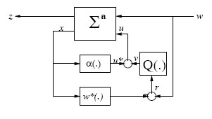
FIGURE 5.2
Controller Parametrization for FI-State-Feedback Nonlinear ${\mathcal{H}}_{\infty }$ -Control

5.1.2    Controller Parametrization

In this subsection, we discuss the state-feedback ${\mathcal{H}}_{\infty }$ controller parametrization problem which deals with the problem of specifying a set (or all the sets) of possible state-feedback controllers that solves the SFBNLHICP for the system (5.1) locally.

The basis for the controller parametrization we discuss is the Youla (or Q)-parametrization for all stabilizing controllers for the linear problem [92, 195, 292] which has been extended to the nonlinear case [188, 215, 214]. Although the original Youla-parametrization uses coprime factorization, the modified version presented in [92] does not use coprime-factorization. The structure of the prametrization is shown in Figure 5.2. Its advantage is that it is given in terms of a free parameter which belongs to a linear space, and the closed-loop map is affine in this free parameter. Thus, this gives an additional degree-of-freedom to further optimize the closed-loop maps in order to achieve other design objectives.

Now, assuming Σ^a is smoothly-stabilizable and the disturbance signal w ∈ ${ℒ}_2$[0, ∞) is fully measurable, also referred to as the full-information (FI) structure, then the following proposition gives a parametrization of a family of full-information controllers that solves the SFBNLHICP for Σ^a.

Proposition 5.1.3 Assume the nonlinear system Σ^a is smoothly stabilizable and zero-state detectable. Suppose further, the disturbance signal is measurable and there exists a smooth (local) solution V ≥ 0 to the HJIE (5.12) or inequality (5.24) such that the SFBNLHICP is (locally) solvable. Let $ℱ\mathcal{G}$ denote the set of finite-gain (in the ${ℒ}_2$ sense) asymptotically-stable (with zero input and disturbances) input-affine nonlinear plants, i.e.,

$ℱ\mathcal{G}\triangleq \left\{{\mathrm{\Sigma }}^a|{\mathrm{\Sigma }}^a\left(u=0,w=0\right)isasymptotically-stableandhas{ℒ}_2-gain\le \gamma \right\}.$

Then, the set

${\mathbf{\text{K}}}_{FI}=\left\{u|u=u^{\star }+Q\left(w-w^{\star }\right),Q\in ℱ\mathcal{G},Q:inputs\mapsto outputs\right\}$

(5.27)

is a paremetrization of all FI-state-feedback controllers that solves (locally) the SFBNLHICP for the system Σ^a.

Proof: Apply u ∈ K_FI to the system Σ^a resulting in the closed-loop system:

${\displaystyle {\sum }_{u^{\star }}^a\left(Q\right):\{\begin{array}{l}\dot{x}=f\left(x\right)+g_1\left(x\right)w+g_2\left(x\right)\left(u^{\star }+Q\left(w-w^{\star }\right)\right);x\left(0\right)=x_0\\ z=\left[\begin{array}{l}{h}_1\left(x\right)\\ u\end{array}\right].\end{array}}$

(5.28)

If Q = 0, then the result follows from Theorem 5.1.2 or 5.1.4. So assume Q ≠ 0, and since $Q\in ℱ\mathcal{G},r\triangleq Q\left(w-w^{\star }\right)\in {ℒ}_2[0,\infty )$. Let V ≥ 0 be a (local) solution of (5.12) or (5.24) in N for some γ > 0. Then, differentiating this along a trajectory of the closed-loop system, completing the squares and using (5.12) or (5.24), we have

$\begin{array}{l}\frac{d}{dt}V=V_x\left[f+g_{1}w-g_2{g}_2^T{V}_x^T+g_{2}r\right]\\ =V_{x}f+\frac{1}{2}{V}_x\left[\frac{1}{{\gamma }^2}{g}_1{g}_1^T-g_2{g}_2^T\right]V_x^T+\frac{1}{2}{\Vert h_1\Vert }^2-\frac{1}{2}{\Vert h_1\Vert }^2-\\ \frac{{\gamma }^2}{2}{\Vert w-\frac{1}{{\gamma }^2}{g}_1^T{V}_x^T\Vert }^2+\frac{1}{2}{\gamma }^2{\Vert w\Vert }^2-\frac{1}{2}{\Vert r-g_2^T{V}_x^T\left(x\right)\Vert }^2+\frac{1}{2}{\Vert r\Vert }^2\\ \le \frac{1}{2}{\gamma }^2{\Vert w\Vert }^2-\frac{1}{2}{\Vert h_1\Vert }^2-\frac{1}{2}{\Vert u\Vert }^2+\frac{1}{2}{\Vert r\Vert }^2-\frac{{\gamma }^2}{2}{\Vert w-\frac{1}{{\gamma }^2}{g}_1^T{V}_x^T\Vert }^2.\end{array}$

(5.29)

Now, integrating the above inequality (5.29) from t = t₀ to t = t₁ > t₀, starting from x(t₀) and using the fact that

${\displaystyle {\int }_{t_0}^{t_1}{\Vert r\Vert }^{2}dt}\le {\gamma }^2{{\displaystyle {\int }_{t_0}^{t_1}\Vert w-w^{\star }\Vert }}^{2}dt\forall t_1\ge t_0,\forall w\in \mathcal{W},$

we get

$V\left(x\left(t_1\right)\right)-V\left(x\left(t_0\right)\right)\le {\displaystyle {\int }_{t_0}^{t_1}\frac{1}{2}\left({\gamma }^2{\Vert w\Vert }^2-{\Vert z\Vert }^2\right)dt,\forall x\left(t_0\right),x\left(t_1\right)\in N.}$

(5.30)

This implies that the closed-loop system (5.28) has ${ℒ}_2$-gain ≤ γ from w to z. Finally, the part dealing with local asymptotic-stability can be proven as in Theorems 5.1.2, 5.1.4. □

Remark 5.1.8 Notice that the set $ℱ\mathcal{G}$ can also be defined as the set of all smooth inputaffine plants Q : r ↦ v with the realization

${\mathrm{\Sigma }}_Q:\le \{\begin{array}{l}\dot{\xi }=a\left(\xi \right)+b\left(\xi \right)r\\ \text{υ}=c\left(\xi \right)\end{array}$

(5.31)

where $\xi \in \mathcal{X},a:\mathcal{X}\to V^{\infty }\left(\mathcal{X}\right),b:\mathcal{X}\to {ℳ}^{n\times p},c:\mathcal{X}\to {\Re }^m$ are smooth functions, with a(0) = 0, c(0) = 0, and such that there exists a positive-definite function $\phi :\mathcal{X}\to {\Re }_{+}$ satisfying the bounded-real condition:

${\phi }_{\xi }\left(\xi \right)a\left(\xi \right)+\frac{1}{2{\gamma }^2}{\phi }_{\xi }\left(\xi \right)b\left(\xi \right)b^T\left(\xi \right){\phi }_{\xi }^T\left(\xi \right)+\frac{1}{2}{c}^T\left(\xi \right)c\left(\xi \right)=0.$

5.2    State-Feedback Nonlinear ${\mathcal{H}}_{\infty }$ Tracking Control

In this section, we consider the traditional state-feedback tracking, model-following or servomechanism problem. This involves the tracking of a given reference signal which may be any one of the classes of reference signals usually encountered in control systems, such as steps, ramps, parabolic or sinusoidal signals. The objective is to keep the error between the system output y and the reference signal arbitrarily small. Thus, the problem can be treated in the general framework discussed in the previous section with the penalty variable z representing the tracking error. However, a more elaborate design scheme may be necessary in order to keep the error as desired above.

The system is represented by the model (5.1) with the penalty variable

$z=\left[\begin{array}{l}{h}_1\left(x\right)\\ u\end{array}\right],$

(5.32)

while the signal to be tracked is generated as the output y_m of a reference model defined by

${\mathrm{\Sigma }}_m:\{\begin{array}{l}{\dot{x}}_m=f_m\left(x_m\right),x_m\left(t_0\right)=x_{m0}\\ y_m=h_m\left(x_m\right)\end{array}$

(5.33)

x_m ∈ ℜ ^l, f_m : ℜ^l → V ^∞(ℜ^l), h_m : ℜ^l → ℜ ^m and we assume that this system is completely observable [212]. The problem can then be defined as follows.

Definition 5.2.1 (State-Feedback Nonlinear ${\mathcal{H}}_{\infty }$ (Suboptimal) Tracking Control Problem (SFBNLHITCP)). Find if possible, a static state-feedback control function of the form

$u={\alpha }_{trk}\left(x,x_m\right),{\alpha }_{trk}:N_O\times N_m\to {\Re }^p$

(5.34)

N_o ⊂ $\mathcal{X}$, N_m ⊂ ℜ^l, for some smooth function α_trk, such that the closed-loop system (5.1), (5.34), (5.33) has, for all initial conditions starting in N_o × N_m neighborhood of (0, 0), locally ${ℒ}_2$-gain from the disturbance signal w to the output z less than or equal to some prescribed number γ^$\star$ > 0 and the tracking error satisfies lim_t→∞{y − y_m} = 0.

To solve the above problem, we follow a two-step procedure:

Step 1: Find a feedforward-control law $u_{\star }=u_{\star }\left(x,x_m\right)$ so that the equilibrium point x = 0 of the closed-loop system

$\dot{x}=f\left(x\right)+g_2\left(x\right)u_{\star }\left(x,0\right)$

(5.35)

is exponentially stable, and there exists a neighborhood U = N_o × N_m of (0, 0) such that for all initial conditions (x₀, x_m0) ∈ U the trajectories (x(t), x_m(t)) of

$\{\begin{array}{l}\dot{x}=f\left(x\right)+g2\left(x\right)u_{\star }\left(x,x_m\right)\\ {\dot{x}}_m=f_m\left(x_m\right)\end{array}$

(5.36)

satisfy

$\underset{t\to \infty }{\lim }\left\{h_1\left(\theta \left(x_m\left(t\right)\right)\right)-h_m\left(x_m\left(t\right)\right)\right\}=0.$

To solve this step, we seek for an invariant-manifold

$M_{\theta }=\left\{x|x=\theta \left(x_m\right)\right\}$

and a control law $u_{\star }={\alpha }_f\left(x,x_m\right)$ such that the submanifold M_θ is invariant under the closed-loop dynamics (5.36) and h₁(θ(x_m(t))) − h_m(x_m(t)) ≡ 0. Fortunately, there is a wealth of literature on how to solve this problem [143]. Under some suitable assumptions, the following equations give necessary and sufficient conditions for the solvability of this problem:

$\frac{\partial \theta }{\partial x_m}\left(x_m\right)(f_m\left(x_m\right)=f\left(\theta \left(x_m\right)\right)+g_2(\theta \left(x_m\right){\overline{u}}_{\star }\left(x_m\right)$

(5.37)

$h_1(\theta \left(x_m\left(t\right)\right)-h_m\left(x_m\left(t\right)\right)=0,$

(5.38)

where ${\overline{u}}_{\star }\left(x_m\right)={\alpha }_f\left(\theta \left(x_m\right),x_m\right)$.

The next step is to design an auxiliary feedback control v so as to drive the system onto the above submanifold and to achieve disturbance-attenuation as well as asymptotic tracking. To formulate this step, we consider the combined system

$\{\begin{array}{l}\dot{x}=f\left(x\right)+g1\left(x\right)w+g2\left(x\right)u\\ {\dot{x}}_m=f_m\left(x_m\right),\end{array}$

(5.39)

and introduce the following change of variables

$\xi =x-\theta \left(x_m\right)$

$\text{υ = }u-{\overline{u}}_{\star }\left(x_m\right).$

Then

$\dot{\xi }=F\left(\xi ,x_m\right)+G_1\left(\xi ,x_m\right)w+G_2\left(\xi ,x_m\right)\text{υ}$

${\dot{x}}_m=f_m\left(x_m\right)$

where

$\begin{array}{l}F\left(\xi ,x_m\right)=f\left(\xi +\theta \left(x_m\right)\right)-\frac{\partial \theta }{\partial x_m}\left(x_m\right)f_m\left(x_m\right)+g_2\left(\xi +\theta \left(x_m\right)\right){\overline{u}}_{\star }\left(x_m\right)\\ G_1\left(\xi ,x_m\right)=g_1\left(\xi +\theta \left(x_m\right)\right)\\ G_2\left(\xi ,x_m\right)=g_2\left(\xi +\theta \left(x_m\right)\right).\end{array}$

Similarly, we redefine the tracking error and the new penalty variable as

$\tilde{z}=\left[\begin{array}{l}{h}_1\left(\xi +\theta \left(x_m\right)\right)-h_m\left(x_m\right)\hfill \\ \text{υ}\hfill \end{array}\right].$

Step 2: Find an auxiliary feedback control ${\upsilon }_{\star }={\upsilon }_{\star }\left(\xi ,x_m\right)$ so that along any trajectory (ξ(t), x_m(t)) of the closed-loop system (5.40), the ${ℒ}_2$-gain condition

$\begin{array}{l}{\displaystyle {\int }_{t_0}^T\Vert \tilde{z}\left(t\right){\Vert }^{2}dt\le {\gamma }^2{\displaystyle {\int }_{t_0}^T\Vert w\left(t\right){\Vert }^{2}dt+\kappa \left(\xi \left(t_0\right),x_{m0}\right)}}\hfill \\ \iff {\displaystyle {\int }_{t_0}^T\left\{\Vert h_1\left(\xi +\theta \left(x_m\right)\right)-h_m\left(x_m\right){\Vert }^2+\Vert \text{υ}{\Vert }^2\right\}dt\le {\gamma }^2{\displaystyle {\int }_{t_0}^T\Vert w\left(t\right){\Vert }^{2}dt+\kappa \left(\xi \left(t_0\right),x_{m0}\right)}}\hfill \end{array}$

is satisfied for some function κ, for all w ∈$\mathcal{W}$, for all T < ∞ and all initial conditions (ξ(t₀), x_m0) in a neighborhood ${\overline{N}}_o$ × N_m of the origin (0, 0). Moreover, if ξ(t₀) = 0 and w(t) ≡ 0, then we may set ${\upsilon }_{\star }\left(t\right)\equiv 0$ to achieve perfect tracking.

Clearly, the above problem is now a standard state-feedback ${\mathcal{H}}_{\infty }$-control problem, and the techniques discussed in the previous sections can be employed to solve it. The following theorem then summarizes the solution to the SFBNLHITCP.

Theorem 5.2.1 Consider the nonlinear system (5.1) and the SFBNLHITCP for this system. Suppose the control law $u_{\star }=u_{\star }\left(x,x_m\right)$ and invariant-manifold M_θ can be found that solve Step 1 of the solution to the tracking problem. Suppose in addition, there exists a smooth solution $\mathrm{\Psi }:{\overline{N}}_o\times N_m\to \Re ,\mathrm{\Psi }\left(\xi ,x_m\right)\ge 0$ to the HJI-inequality

$\begin{array}{l}{\mathrm{\Psi }}_{\xi }\left(\xi ,x_m\right)F\left(\xi ,x_m\right)+{\mathrm{\Psi }}_{x_m}\left(\xi ,x_m\right)f_m\left(x_m\right)+\\ \frac{1}{2}{\mathrm{\Psi }}_{\xi }\left(\xi ,x_m\right)\left[\frac{1}{{\gamma }^2}{G}_1\left(\xi ,x_m\right)G_1^T\left(\xi ,x_m\right)-G_2\left(\xi ,x_m\right)G_2^T\left(\xi ,x_m\right)\right]{\mathrm{\Psi }}_{\xi }^T\left(\xi ,x_m\right)+\\ \frac{1}{2}{\Vert h_1\left(\xi +x_m\right)-h_m\left(x_m\right)\Vert }^2\le 0,x\in {\overline{N}}_o,\xi \in N_m,\mathrm{\Psi }\left(0,0\right)=0.\end{array}$

(5.40)

Then the SFBNLHITCP is locally solvable with the control laws u = ${\overline{u}}_{\star }$ and

${\upsilon }_{\star }=-G_2^T\left(\xi ,x_m\right){\mathrm{\Psi }}_{\xi }^T\left(\xi ,x_m\right).$

Moreover, if Ψ is proper with respect to ξ (i.e., if Ψ(ξ, x_m) → ∞ when $\Vert \xi \Vert$ → ∞) and the system is zero-state detectable, then lim_{t →∞} ξ(t) = 0 also for all initial conditions $\left(\xi \left(t_0\right),x_{m0}\right)\in {\overline{N}}_0\times N_m$.