6

Output-Feedback Nonlinear ${\mathcal{H}}_{\infty }$-Control for Continuous-Time Systems

In this chapter, we discuss the nonlinear ${\mathcal{H}}_{\infty }$ sub-optimal control problem for continuous-time nonlinear systems using output-feedback. This problem arises when the states of the system are not available for feedback, and so have to be estimated in some way and then used for feedback, or the output of the system itself is used for feedback. The estimator is basically an observer that satisfies an ${\mathcal{H}}_{\infty }$ requirement. In the former case, the observer uses the measured output of the system to estimate the states, and the whole arrangement is referred to as an observer-based controller or more generally a dynamic controller. The set-up is depicted in Figure 6.1 in this case. For the most part, this chapter will be devoted to this problem. On the other hand, the latter problem is referred to as a static output-feedback controller and will be discussed in the last section of the chapter.

We derive sufficient conditions for the solvability of the above problem for time-invariant (or autonomous) affine nonlinear systems, as well as for a general class of systems. The parametrization of stabilizing controllers is also discussed. The problem of robust control in the presence of modelling errors and/or parameter variations is also considered, as well as the reliable control of sytems in the event of sensor and/or actuator failure.

6.1    Output Measurement-Feedback ${\mathcal{H}}_{\infty }$-Control for Affine Nonlinear Systems

We begin in this section with the output-measurement feedback problem in which it is desired to synthesize a dynamic observer-based controller using the output measurements. To this effect, we consider first an affine causal state-space system defined on a smooth n-dimensional manifold $\mathcal{X}\subseteq {\Re }^n$in local coordinates x = (x₁,…, x_n):

${\mathrm{\Sigma }}^a:\{\begin{array}{l}\dot{x}=f\left(x\right)+g_1\left(x\right)w+g_2\left(x\right)u;x\left(t_0\right)=x_0\\ z=h_1\left(x\right)+k_{11}\left(x\right)w+k_{12}\left(x\right)u\\ y=h_2\left(x\right)+k_{21}\left(x\right)w\end{array}$

(6.1)

where $x\in \mathcal{X}$ is the state vector, $u\in \mathcal{U}\subseteq {\Re }^p$ is the p-dimensional control input, which belongs to the set of admissible controls $\mathcal{U},w\in \mathcal{W}$ is the disturbance signal, which belongs to the set $\mathcal{W}\subset {\mathcal{L}}_2([t_0,\infty ){\Re }^r)$ of admissible disturbances, the output $y\in \mathcal{Y}\subset {\Re }^m$ is the measured output of the system, and $z\in {\Re }^s$ is the output to be controlled. The functions $f:\mathcal{X}\to V^{\infty }(\mathcal{X}),g_1:\mathcal{X}\to {\mathcal{M}}^{n\times r}(\mathcal{X}),g_2:\mathcal{X}\to {\mathcal{M}}^{n\times p}(\mathcal{X}),h_1:\mathcal{X}\to {\Re }^s,h_2:\mathcal{X}\to {\Re }^m$, and $k_{11}:\mathcal{X}\to {\mathcal{M}}^{s\times r},k_{12}:\mathcal{X}\to {\mathcal{M}}^{s\times p}(\mathcal{X}),k_{21}:\mathcal{X}\to {\mathcal{M}}^{m\times r}(\mathcal{X})$ are real C^∞ functions of x. Furthermore, we assume without any loss of generality that the system (6.1) has a unique equilibrium-point at x = 0 such that f(0) = 0, h₁(0) = h₂(0) = 0, and for simplicity we have the following assumptions which are the nonlinear versions of the standing assumptions in [92]:

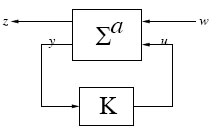
FIGURE 6.1
Configuration for Nonlinear ${\mathcal{H}}_{\infty }$-Control with Measurement-Feedback

Assumption 6.1.1 The system matrices are such that

$\begin{array}{l}{k}_{11}\left(x\right)=0\\ h_1^T\left(x\right)k_{12}\left(x\right)=0\\ k_{12}^T\left(x\right)k_{12}\left(x\right)=I\\ k_{21}\left(x\right)g_1^T\left(x\right)=0\\ k_{21}\left(x\right)k_{21}^T\left(x\right)=I.\end{array}\}.$

(6.2)

Remark 6.1.1 The first of these assumptions corresponds to the case in which there is no direct feed-through between w and z; while the second and third ones mean that there are no cross-product terms and the control weighting matrix is identity in the norm function for z respectively. Lastly, the fourth and fifth ones are dual to the second and third ones.

We begin with the following definition.

Definition 6.1.1 (Measurement-Feedback (Sub-Optimal) ${\mathcal{H}}_{\infty }$-Control Problem (MFBNLHICP)). Find (if possible!) a dynamic feedback-controller of the form:

${\displaystyle {\sum }_{dyn}^c:}\{\begin{array}{l}\dot{\text{ξ}}\text{=}\eta \left(\xi ,y\right)\\ u=\theta \left(\xi ,y\right),\end{array}$

(6.3)

where $\xi \in \text{Ξ}\subset \mathcal{X}$ a neighborhood of the origin, and $\eta :\text{Ξ}\times {\Re }^m\to V^{\infty }\left(\text{Ξ}\right),\eta \left(0,0\right)=0,\theta :\text{Ξ}\times {\Re }^m\to {\Re }^p,\theta \left(0,0\right)=0$, are some smooth functions, which processes the measured variable y of the plant (6.1) and generates the appropriate control action u, such that the closed-loop system (6.1), (6.3) has locally ${\mathcal{L}}_2$-gain from the disturbance signal w to the output z less than or equal to some prescribed number γ^⋆ > 0 with internal stability, or equivalently, the closed-loop system achieves local disturbance-attenuation less than or equal to γ^⋆ with internal-stability.

Since the state information is not available for measurement in contrast with the previous chapter, the simplest thing to do is to estimate the states with an observer, and then use this estimate for feedback. From previous experience on the classical theory of state observation, the “estimator” usually comprises of an exact copy of the dynamics of x, corrected by a term proportional to the error between the actual output y of the plant (6.1) and an estimated output ŷ. Such a system can be described by the equations:

${\displaystyle {\sum }_e^c:\{\begin{array}{l}\dot{\text{ξ}}\text{=}f\left(\xi \right)+g_1\left(\xi \right)w+g_2\left(\xi \right)u+G\left(\xi \right)\left(y-\widehat{y}\right)\\ \widehat{y}=h_2\left(\xi \right)+k_{21}\left(\xi \right)w,\end{array}}$

(6.4)

where G(.) is the output-injection gain matrix which is to be determined. A state-feedback control law can then be imposed on the system based on this estimated state (and the results from Chapter 5) as:

$u:={\alpha }_2\left(\xi \right)=-g_2^T\left(\xi \right)V_{\xi }^T\left(\xi \right),$

(6.5)

where V solves the HJIE (5.12). The combination of (6.4) and (6.5) will then represent our postulated dynamic-controller (6.3). With the above feedback, the estimator (6.4) becomes

$\dot{\xi }=f\left(\xi \right)+g_1\left(\xi \right)w+g_2\left(\xi \right){\alpha }_2\left(\xi \right)+G\left(\xi \right)\left(y-\widehat{y}\right).$

(6.6)

Besides the fact that we still have to determine an appropriate value for G(.), we also require an explicit knowledge of the disturbance w. Since the knowledge of w is generally not available, it is reasonable to replace its actual value by the “worst-case” value, which is given (from Chapter 5) by

$w^{\star }:={\alpha }_1\left(x\right)=\frac{1}{{\gamma }^2}{g}_1^T\left(x\right)V_x^T\left(x\right)$

for some γ > 0. Substituting this expression in (6.6) and replacing x by ξ, results in the following certainty-equivalence worst-case estimator

$\dot{\xi }=f\left(\xi \right)+g_1\left(\xi \right){\alpha }_1\left(\xi \right)+g_2\left(\xi \right){\alpha }_2\left(\xi \right)+G\left(\xi \right)\left(y-h_2\left(\xi \right)-k_{21}\left(\xi \right){\alpha }_1\left(\xi \right)\right).$

(6.7)

Next, we return to the problem of selecting an appropriate gain matrix G(.), which is another of our design parameters, to achieve the objectives stated in Definition 6.1.1. It will be shown in the following that, if some appropriate sufficient conditions are fulfilled, then the matrix G(.) can be chosen to achieve this.

We begin with the closed-loop system describing the dynamics of the plant (6.1) and the dynamic-feedback controller (6.7), (6.5) which has the form

${\displaystyle \sum }_{clp}^{ac}:\{\begin{array}{l}\dot{x}=f\left(x\right)+g_1\left(x\right)w+g_2\left(x\right){\alpha }_2\left(\xi \right);x\left(t_0\right)=x_0\hfill \\ \dot{\xi }=\tilde{f}\left(\xi \right)+g_2\left(\xi \right)+G\left(\xi \right)\left(h_2\left(x\right)+k_{21}\left(x\right)w-{\tilde{h}}_2\left(\xi \right)\right)\hfill \\ z=h_1\left(x\right)+k_{12}\left(x\right){\alpha }_2\left(\xi \right)\hfill \end{array}$

(6.8)

where

$\begin{array}{l}\tilde{f}\left(\xi \right)=f\left(\xi \right)+g_1\left(\xi \right){\alpha }_1\left(\xi \right)\\ {\tilde{h}}_2\left(\xi \right)=h_2\left(\xi \right)+k_{21}\left(\xi \right){\alpha }_1\left(\xi \right).\end{array}$

If we can choose G(.) such that the above closed-loop system (6.8) is dissipative with a C¹ storage-function, with respect to the supply-rate $s\left(w,z\right)=\frac{1}{2}\left({\gamma }^2{\Vert w\Vert }^2-{\Vert z\Vert }^2\right)$ and is locally asymptotically-stable about (x, ξ) = (0, 0), then we would have solved the MFBNLHICP for (6.1).

To proceed, let us further combine the x and ξ dynamics in the dynamics x^e as follows.

${\dot{x}}^e=f^e\left(x^e\right)+g^e\left(x^e\right)\left(w-{\alpha }_1\left(x\right)\right)$

(6.9)

where

$\begin{array}{l}{x}^e=\left(\begin{array}{l}x\\ \xi \end{array}\right),f^e\left(x^e\right)=\left(\begin{array}{l}\tilde{f}\left(x\right)+g_2\left(x\right){\alpha }_2\left(\xi \right)\\ \tilde{f}\left(x\right)+g_2\left(x\right){\alpha }_2\left(\xi \right)+G\left(\xi \right)\left(h_2\left(x\right)-{\tilde{h}}_2\left(\xi \right)\right)\end{array}\right),\\ g^e\left(x^e\right)=\left(\begin{array}{l}{g}_1\left(x\right)\\ G\left(\xi \right){\kappa }_{21}\left(x\right)\end{array}\right),\end{array}$

and let

$h^e\left(x^e\right)={\alpha }_2\left(x\right)-{\alpha }_2\left(\xi \right).$

Apply now the change of input variable r = w − α₁(x) in (6.9) and set the output to v obtaining the following equivalent system:

$\{\begin{array}{l}{\dot{x}}^e=f^e\left(x^e\right)+g^e\left(x^e\right)r\\ v=h^e\left(x^e\right).\end{array}$

(6.10)

The problem would then be solved if we can choose G(.) such that the above system (6.10) is dissipative with respect to the supply-rate $s\left(r,v\right)=\frac{1}{2}\left({\gamma }^2{\Vert r\Vert }^2-{\Vert v\Vert }^2\right)$ and internally-stable. A necessary and sufficient condition for this to happen is if the following bounded-real condition [139] is satisfied:

$W_{x^e}\left(x^e\right)f^e\left(x^e\right)+\frac{1}{2{\gamma }^2}{W}_{x^e}\left(x^e\right)g^e\left(x^e\right)g^e{}^T\left(x^e\right)W_{x^e}^T\left(x^e\right)+\frac{1}{2}{h}^{eT}\left(x^e\right)h^e\left(x^e\right)\le 0$

(6.11)

for some C¹ nonnegative function $W:N\times N\to \Re$

locally defined in a neighborhood $N\subset \mathcal{X}$ of x^e = 0, and which vanishes at x^e = 0. The above inequality further implies that

$W_{x^e}\left(x^e\right)\left(f^e\left(x^e\right)+g^e\left(x^e\right)r\right)\le \frac{1}{2}\left({\gamma }^2{\Vert r\Vert }^2-{\Vert v\Vert }^2\right)\forall r\in W,$

(6.12)

which means, W is a storage-function for the equivalent system with respect to the supply-rate $s\left(r,v\right)=\frac{1}{2}\left({\gamma }^2{\Vert r\Vert }^2-{\Vert v\Vert }^2\right).$ Now assuming that W exists, then it can be seen that the closed-loop system (6.8) is locally dissipative, with the storage-function

$\mathrm{\Psi }\left(x^e\right)=V\left(x\right)+W\left(x^e\right),$

with respect to the supply-rate $s\left(w,z\right)=\frac{1}{2}\left({\gamma }^2{\Vert w\Vert }^2-{\Vert z\Vert }^2\right),$, where V (.) solves the HJIE(5.12). Indeed,

$\begin{array}{l}\frac{d\mathrm{\Psi }\left(x^e\left(t\right)\right)}{dt}+\frac{1}{2}\left({\Vert z\Vert }^2-{\gamma }^2{\Vert w\Vert }^2\right)={\mathrm{\Psi }}_{x^e}\left(f^e\left(x^e\right)+g^e\left(x^e\right)\left(w-{\alpha }_1\left(x\right)\right)\right)+\frac{1}{2}\left({\Vert z\Vert }^2-{\gamma }^2{\Vert w\Vert }^2\right)\\ =V_x\left(x\right)\left(f\left(x\right)+g_1\left(x\right)w+g_2\left(x\right){\alpha }_2\left(\xi \right)\right)+\\ W_{x^e}\left(f^e\left(x^e\right)+g^e\left(x^e\right)r\right)+\frac{1}{2}{\Vert h_1\left(x\right)+k_{12}\left(x\right){\alpha }_2\left(\xi \right)\Vert }^2\\ -\frac{1}{2}{\gamma }^2{\Vert w\Vert }^2\\ \le \frac{1}{2}\left\{{\Vert {\alpha }_2\left(\xi \right)-{\alpha }_2\left(x\right)\Vert }^2-{\gamma }^2{\Vert w-{\alpha }_1\left(x\right)\Vert }^2+{\gamma }^2{\Vert r\Vert }^2-{\Vert v\Vert }^2\right\}\\ \le 0,\end{array}$

which proves dissipativity. The next step is to show that the closed-loop system (6.9) has a locally asymptotically-stable equilibrium-point at (x, ξ) = (0, 0). For this, we need additional assumptions on the system (6.1).

Assumption 6.1.2 Any bounded trajectory x(t) of the system

$\dot{x}\left(t\right)=f\left(x\left(t\right)\right)+g_2\left(x\left(t\right)\right)u\left(t\right)$

satisfying

$h_1\left(x\left(t\right)\right)+k_{12}\left(x\left(t\right)\right)u\left(t\right))=0$

for all t≥t_s, is such that ${\lim }_{t\to \infty }x\left(t\right)=0.$

Assumption 6.1.3 The equilibrium-point ξ = 0 of the system

$\dot{\xi }=\tilde{f}\left(\xi \right)-G\left(\xi \right){\tilde{h}}_2\left(\xi \right)$

(6.13)

is locally asymptotically-stable.

Then from above, with w = 0,

$\begin{array}{l}\frac{d\mathrm{\Psi }\left(x^e\left(t\right)\right)}{dt}={\mathrm{\Psi }}_{x^e}\left(f^e\left(x^e\right)+g^e\left(x^e\right)\left(-{\alpha }_1\left(x\right)\right)\right)\\ \le -\frac{1}{2}{\Vert h{}_1\left(x\left(t\right)\right)+k_{12}\left(x\left(t\right)\right){\alpha }_2\left(\xi \left(t\right)\right)\Vert }^2\end{array}$

(6.14)

along any trajectory (x(.), ξ(.)) of the closed-loop system. This proves that the equilibrium-point (x(.), ξ(.)) = (0, 0) is stable. To prove asymptotic-stability, observe that any trajectory x^e(t) such that

$\frac{d\mathrm{\Psi }\left(x^e\left(t\right)\right)}{dt}\equiv 0,\forall t\ge t_s,$

is necessarily a trajectory of

$\dot{x}=f\left(x\right)+g_2\left(x\right){\alpha }_2\left(\xi \right)$

such that x(t) is bounded and

$h_1\left(x\left(t\right)\right)+k_{12}\left(x\left(t\right)\right){\alpha }_2\left(\xi \left(t\right)\right)\equiv 0$

for all t≥t_s. By Assumption 6.1.2, this implies lim_t→∞ x(t) = 0. Moreover, since k₁₂(x) has full column rank, the above also implies that lim_t→∞ α₂(ξ(t)) = 0. Thus, the ω-limit set of such a trajectory is a subset of

${\mathrm{\Omega }}_0=\left\{\left(x,\xi \right)|x=0,{\alpha }_2\left(\xi \right)=0\right\}.$

Any initial condition on this limit-set yields a trajectory

$x\left(t\right)\equiv 0$

for all t≥t_s, which corresponds to the trajectory ξ(t) of

$\dot{\xi }=\tilde{f}\left(\xi \right)-G\left(\xi \right){\tilde{h}}_2\left(\xi \right).$

By Assumption 6.1.3, this implies lim_t→∞ ξ(t) = 0, and local asymptotic-stability follows from the invariance-principle.

The above result can now be summarized in the following lemma.

Theorem 6.1.1 Consider the nonlinear system (6.1) and suppose Assumptions 6.1.1, 6.1.2 hold. Suppose also there exists a C¹ positive-(semi)definite function $V:N\to {\Re }_{+}$ locally defined in a neighborhood N of x = 0, vanishing at x = 0 and satisfying the HJIE (5.12). Further, suppose there exists also a C¹ real-valued function $W:N_1\times N_1\to \Re$ locally defined in a neighborhood N₁ × N₁ of x^e = 0, vanishing at x^e = 0 and is such that W (x^e) > 0 for all x ≠ ξ, together with an n × m smooth matrix function $G(\xi ):N_2\to {\mathcal{M}}^{n\times m}$, locally defined in a neighborhood N₂ of ξ = 0, such that

(i)	the HJIE (6.11) holds;
(ii)	Assumption 6.1.3 holds;
(iii)	N ∩ N1 ∩ N2 = ∅.

Then the MFBNLHICP for the system (6.1) is locally solvable.

A modified result to the above Theorem 6.1.1 as given in [141, 147] can also be proven along the same lines as the above. We first have the following definition.

Definition 6.1.2 Suppose f(0) = 0, h(0) = 0, then the pair {f, h} is locally zero-state detectable, if there exists a neighborhood O of x = 0 such that, if x(t) is a trajectory of the free-system $\dot{x}$ = f(x) with x(t₀) ∈ O, then h(x(t)) is defined for all t ≥ 0 and h(x(t)) ≡ 0 for all t ≥ t₀, implies lim_t→∞ x(t) = 0

Theorem 6.1.2 Consider the nonlinear system (6.1) and assume that $k_{21}(x)k_{21}^T(x)=I$ in (6.2). Assume also the following:

(i)  The pair {f, h₁} is locally zero-state detectable.

(ii)  There exists a smooth positive-(semi)definite function V locally defined in a neighborhood N of the origin x = 0 with V (0) = 0 and satisfying the HJIE (5.12).

(iii)  There exists an n × m smooth matrix function G(ξ) such that the equilibrium-point ξ = 0 of the system

$\dot{\xi }=f\left(\xi \right)-g_1\left(\xi \right){\alpha }_1\left(\xi \right)-G\left(\xi \right)h_2\left(\xi \right).$

(6.15)

is locally asymptotically-stable.

(iv)   There exists a smooth positive-semidefinite function W (x, ξ) locally defined in a neighborhood $N_1\times N_1\subset \mathcal{X}\times \mathcal{X}$ of the origin such that W (0, ξ) > 0 for each ξ ≠ 0, and satisfying the HJIE :

$\begin{array}{l}\left[W_x\left(x,\xi \right)W_{\xi }\left(x,\xi \right)\right]f_e\left(x,\xi \right)+\\ \frac{1}{2{\gamma }^2}\left[W_x\left(x,\xi \right)W_{\xi }\left(x,\xi \right)\right]\left[\begin{array}{cc}{g}_1\left(x\right)g_1^T\left(x\right)& 0\\ 0& G\left(\xi \right)G^T\left(\xi \right)\end{array}\right]\left[\begin{array}{l}{W}_x^T\left(x,\xi \right)\\ W_{\xi }^T\left(x,\xi \right)\end{array}\right]+\\ \frac{1}{2}{h}_e^T\left(x,\xi \right)h_e\left(x,\xi \right)=0,W\left(0,0\right)=0,\left(x,\xi \right)\in N_1\times N_1.\end{array}$

(6.16)

Then, the MFBNLHICP for the system is solved by the output-feedback controller:

${\displaystyle {\sum }_2^c:\{\begin{array}{l}\dot{\xi }=f\left(\xi \right)+g_1\left(\xi \right){\alpha }_1\left(\xi \right)+g_2\left(\xi \right){\alpha }_2\left(\xi \right)+G\left(\xi \right)\left(y-h_2\left(\xi \right)\right)\\ u={\alpha }_2\left(\xi \right),\end{array}}$

(6.17)

where f_e(x, ξ), h_e(x, ξ), are given by:

$\begin{array}{l}{f}_e\left(x,\xi \right)=\left(\begin{array}{l}f\left(x\right)+g_1\left(x\right){\alpha }_1\left(x\right)+g_2\left(x\right){\alpha }_2\left(\xi \right)\\ f\left(\xi \right)+g_1\left(\xi \right){\alpha }_1\left(\xi \right)+g_2\left(\xi \right)+G\left(\xi \right)\left(h_2\left(x\right)-h_2\left(\xi \right)\right)\end{array}\right)\\ h_e\left(x,\xi \right)={\alpha }_2\left(\xi \right)-{\alpha }_2\left(x\right).\end{array}$

Example 6.1.1 We specialize the result of Theorem 6.1.2 to linear systems and compare it with some standard results obtained in other references, e.g., [92] (see also [101, 292]). Consider the linear time-invariant system (LTI):

${\mathrm{\Sigma }}^l\text{}:\{\begin{array}{l}\dot{x}=Fx+G_{1}w+G_{2}u\\ z=H_{1}x+K_{12}u\\ y=H_{2}x+K_{21}w\end{array}$

(6.18)

for constant matrices $F\in {\Re }^{n\times n},G_1\in {\Re }^{n\times r},G_2\in {\Re }^{n\times p},H_1\in {\Re }^{s\times n},H_2\in {\Re }^{m\times n}$ $K_{12}\in {\Re }^{s\times p}$ and $K_{21}\in {\Re }^{m\times r}$ satisfying Assumption 6.1.1. Then, we have the following result.

Proposition 6.1.1 Consider the linear system (6.18) and suppose the following hold:

(a)  the pair (F, G₁) is stabilizable;

(b)  the pair (F, H₁) is detectable;

(c)  there exist positive-definite symmetric solutions X, Y of the AREs:

$F^{T}X+XF+X\left[\frac{1}{{\gamma }^2}{G}_1{G}_1^T-G_2{G}_2^T\right]+H_1^T{H}_1=\mathrm{0,}$

(6.19)

${\text{Y F}}^T+FY+Y\left[\frac{1}{{\gamma }^2}{H}_1{H}_1^T-H_2{H}_2^T\right]+G_1^T{G}_T=0;$

(6.20)

(d)  $\rho (XY)<{\gamma }^2$

Then, the hypotheses (i)-(iv) in Theorem 6.1.2 also hold, with

$\begin{array}{l}G=Z{H}_2^T\\ V(x)=\frac{1}{2}{x}^T{X}_x\\ \text{W(}x,\xi \text{)}\text{= }\frac{1}{2}{\gamma }^2(x-\xi )Z^{-1}(x-\xi ),\end{array}$

where

$Z=Y{\left(I-\frac{1}{{\gamma }^2}XY\right)}^{-1}$

Proof: (i) is identical to (b). To show (ii) holds, we note that, if X is a solution of the ARE (6.19), then the positive-definite function $V(x)=\frac{1}{2}{x}^{T}Xx$ is a solution of the HJIE (6.16). To show that (iii) holds, observe that, if X is a solution of ARE (6.19) and Y a solution of ARE (6.20), then the matrix

$Z=Y{\left(I-\frac{1}{{\gamma }^2}XY\right)}^{-1}$

is a solution of the ARE [292]:

$Z{\left(F+G_1{F}_1\right)}^T+\left(F+G_1{F}_1\right)Z+Z\left(\frac{1}{{\gamma }^2}{F}_2^T{F}_2-H_2^T{H}_2\right)Z+G_1{G}_1^T=0,$

(6.21)

where $F_1=\frac{1}{{\gamma }^2}{G}_1^{T}X$ and $F_2=G_2^{T}X$. Moreover, Z is symmetric and by hypothesis (d) Z is positive-definite. Hence we can take V (ξ) = ξ^T Z ξ as a Lyapunov-function for the system

$\dot{\xi }={\left(F+G_1{F}_1-G{H}_2\right)}^T\xi ,$

(6.22)

which is the linear equivalent of (6.15). Using the ARE (6.21), it can be shown that

$\dot{L}=-\left({\Vert G^T\xi \Vert }^2+\Vert G_1^T\xi \Vert +\frac{1}{{\gamma }^2}{\Vert F_{2}Z\xi \Vert }^2\right),$

which implies that the equilibrium-point ξ = 0 for the system (6.22) is stable. Furthermore, the condition $\dot{L}(\xi (t))=0$ implies G₁ξ(t) = 0 and G ξ(t) = 0, which results in

$\stackrel{\text{.}}{\text{ξ}}\left(t\right)=F^T\xi \left(t\right).$

Finally, since (A, G₁) is stabilizable, together with the fact that G₁ξ(t) = 0, and the standard invariance-principle, we conclude that lim_t→∞ ξ(t) = 0 or asymptotic-stability of the system (6.22). Thus, (iii) also holds.

Lastly, it remains to show that (iv) also holds. Choosing

$W\left(x,\xi \right)=\frac{1}{2}{\gamma }^2{\left(x-\xi \right)}^T{Z}^{-1}\left(x-\xi \right)$

and substituting in the HJIE (6.16), we get four AREs which are all identical to the ARE (6.21), and the result follows. □

Remark 6.1.2 Based on the result of the above proposition, it follows that the linear dynamic-controller

$\begin{array}{l}\dot{\xi }=\left(F+G_1{F}_1+G_2{F}_2-G{H}_2\right)\xi +Gy\\ u=F_2\xi \end{array}$

with $F_1=\frac{1}{{\gamma }^2}{G}_1^{T}X,F_2=-G_2^{T}X$ and $G=Z{H}_2^T$ solves the linear MFBNLHICP for the system (6.18)

The preceding results, Theorems 6.1.1, 6.1.2, establish sufficient conditions for the solvability of the output measurement-feedback problem. However, they are not satisfactory in that, firstly, they do not give any hint on how to select the output-injection gain-matrix G(.) such that the HJIE (6.11) or (6.16) is satisfied and the closed-loop system (6.13) is locally asymptotically-stable. Secondly, the HJIEs (6.11), (6.16) have twice as many independent variables as the HJIE (5.12). Thus, a final step in the above design procedure would be to partially address these concerns.

Accordingly, an alternative set of sufficient conditions can be provided which involve an additional HJI-inequality having the same number of independent variables as the dimension of the plant and not involving the gain matrix G(.). For this, we begin with the following lemma.

Lemma 6.1.1 Suppose V is a C³ solution of the HJIE (5.12) and $Q:O\to \Re$ is a C³ positive-definite function locally defined in a neighborhood of x = 0, vanishing at x = 0 and satisfying

$S\left(x\right)<0$

where

$S\left(x\right)=Q_x\left(x\right)\left(\tilde{f}\left(x\right)-G\left(x\right){\tilde{h}}_2\left(x\right)\right)+\frac{1}{2{\gamma }^2}{Q}_x\left(x\right)\left(g_1\left(x\right)-G\left(x\right)k_{21}\left(x\right)\right){\left(g_1\left(x\right)-G\left(x\right)k_{21}\left(x\right)\right)}^T{Q}_x^T\left(x\right)+\frac{1}{2}{\alpha }_2^T\left(x\right){\alpha }_2\left(x\right),$

for each x ≠ 0 and such that the Hessian matrix $\frac{{\partial }^{2}s}{\partial x^2}$ is nonsingular at x = 0. Then the function

$W\left(x^e\right)=Q\left(x-\xi \right)$

satisfies the conditions (i), (ii) of Theorem 6.1.1.

Proof: Let$W\left(x^e\right)=Q\left(x-\xi \right)$ and let

$\text{ϒ}\left(x,\xi \right)=W_{x^e}\left(x^e\right)f^e\left(x^e\right)+\frac{1}{2{\gamma }^2}{W}_{x^e}\left(x^e\right)g^e\left(x^e\right)g^{eT}\left(x^e\right)W_{x^e}^T(\left(x^e\right)+\frac{1}{2}{h}^{eT}\left(x^e\right)h^e\left(x^e\right).$

Thus, to show that W(.) as defined above satisfies condition (i) of Theorem 6.1.1, is to show that ϒ is nonpositive. For this, set

$e=x-\xi$

and let

$\text{Π}\left(e,\xi \right)={\left[\text{ϒ}\left(x,\xi \right)\right]}_{x=\xi +e^{}}.$

It can then be shown by simple calculations that

$\text{Π}\left(0,\xi \right)=0,{\frac{\partial \prod \left(e,\xi \right)}{\partial e}|}_{e=0}=0,$

which means Π(x, ξ) can be expressed in the form

$\text{Π}\left(e,\xi \right)=e^T\mathrm{\Lambda }\left(e,\xi \right)e$

for some C⁰ matrix function Λ(., .). Moreover, it can also be verified that

$\mathrm{\Lambda }\left(0,0\right)={\frac{{\partial }^{2}S\left(x\right)}{\partial x^2}|}_{x=0}<0$

by assumption. Thus, Π(e, ξ) is nonpositive in the neighborhood of (x, ξ) = (0, 0) and (i) follows.

To establish (ii), note that by hypothesis S(x) < 0 implies

$Q_x\left(x\right)\left(\tilde{f}\left(x\right)-G\left(x\right){\tilde{h}}_2\left(x\right)\right)<0.$

Therefore, Q(x) > 0 is a Lyapunov-function for the system (6.13), and the equilibrium-point ξ = 0 of this system is locally asymptotically-stable. Hence the result. □

As a consequence of the above lemma, we can now present alternative sufficient conditions for the solvability of the MFBNLHICP. We begin with the following assumption.

Assumption 6.1.4 The matrix

$R_1\left(x\right)=k_{21}^T\left(x\right)k_{21}\left(x\right)$

is nonsingular (and positive-definite) for each x.

Theorem 6.1.3 Consider the nonlinear system (6.1) and suppose Assumptions 6.1.1, 6.1.2 and 6.1.4 hold. Suppose also the following hold:

(i)  there exists a C³ positive-definite function V, locally defined in a neighborhood N of x = 0 and satisfying the HJIE (5.12);

(ii)  there exists a C³ positive-definite function $Q:N_1\subset \mathcal{X}\to {\Re }_{+}$ locally defined in a neighborhood N₁ of x = 0, vanishing at x = 0, and satisfying the HJ-inequality

$Q_x\left(x\right)f^{\#}\left(x\right)+\frac{1}{2{\gamma }^2}{Q}_x\left(x\right)g_1^{\#}\left(x\right)g_1^{\#T}\left(x\right)Q_x^T\left(x\right)+\frac{1}{2}{H}^{\#}\left(x\right)<0$

(6.23)

together with the coupling condition

$Q_x\left(x\right)L\left(x\right)={\tilde{h}}_2^T\left(x\right)$

(6.24)

for some n × m smooth C² matrix function L(x), where

$\begin{array}{l}{f}^{\#}\left(x\right)=\tilde{f}\left(x\right)-g_1\left(x\right)k_{21}^T\left(x\right)R_1^{-1}\left(x\right){\tilde{h}}_2\left(x\right),\\ g_1^{\#}\left(x\right)=g_1\left(x\right)\left[I-k_{12}^T\left(x\right)R_1^{-1}\left(x\right)k_{21}\left(x\right)\right],\\ H^{\#}\left(x\right)=\left({\alpha }_2^T\left(x\right){\alpha }_2\left(x\right)-{\gamma }^2\tilde{h}\left(x\right)R_1^{-1}\left(x\right){\tilde{h}}_2\left(x\right)\right),\end{array}$

and such that the Hessian matrix of the right-hand-side of (6.23) is nonsingular for all x ∈ N₁.

Then the MFBNLHICP for the system is solvable with the controller (6.7), (6.5) if G(.) is selected as

$G\left(x\right)=\left({\gamma }^{2}L\left(x\right)+g_1\left(x\right)k_{21}^T\left(x\right)\right)R_1^{-1}\left(x\right).$

(6.25)

Proof: (Sketch, see [139] for details). By standard completion of squares arguments, it can be shown that the function S(x) satisfies the inequality

$\begin{array}{l}S\left(x\right)\ge Q_x\left(x\right)\left(\tilde{f}\left(x\right)-g_1\left(x\right)k_{21}^T\left(x\right)R_1^{-1}\left(x\right){\tilde{h}}_2\left(x\right)\right)+\frac{1}{2}\left[{\alpha }_2^T\left(x\right){\alpha }_2\left(x\right)-{\gamma }^2{\tilde{h}}_2^T\left(x\right){\tilde{h}}_2\left(x\right)\right]+\\ \frac{1}{2{\gamma }^2}Q\left(x\right)g_1\left(x\right)\left[I-K_{21}^T\left(x\right)R_1^{-1}\left(x\right)k_{21}\left(x\right)\right]g_1^T\left(x\right)Q_x^T\left(x\right),\end{array}$

and equality holds if and only if

$Q_x\left(x\right)G\left(x\right)=\left({\gamma }^2{\tilde{h}}_2\left(x\right)+Q_x{g}_1\left(x\right)k_{21}\left(x\right)\right)R_1^{-1}\left(x\right).$

Therefore, in order to make S(x) < 0, it is sufficient for the new HJ-inequality (6.23) to hold for each x and G(x) to be chosen as in (6.25). In this event, the matrix G(x) exists if and only if Q(x) satisfies (6.24). Finally, application of the results of Theorem 6.1.1, Lemma 6.1.1 yield the result. □

Example 6.1.2 We consider the case of the linear system (6.18) in which case the simplifying assumptions (6.2) reduce to:

$K_{12}^T{K}_{12}=I,H_1^T{K}_{12}=0,K_{21}{G}_1^T=0,K_{21}^T{K}_{21}=R_1>0.$

The existence of a C³ positive-definite function Q satisfying the strict HJ-inequality (6.23) is equivalent to the existence of a symmetric positive-definite matrix Z satisfying the bounded-real inequality

$F^{\#T}Z+Z{F}^{\#}+\frac{1}{{\gamma }^2}Z{G}_1^{\#}{G}_1^{\#T}Z+H^{\#}<0$

(6.26)

where

$F^{\#}=\tilde{F}-G_1{K}_{21}^T{R}_1^{-1}{\tilde{H}}_2,G_1^{\#}=G_1\left(I-K_{21}^T{R}_1^{-1}{K}_{21}\right),H^{\#}=F_2^T{F}_2-{\gamma }^2{\tilde{H}}_2^T{R}_1^{-1}{\tilde{H}}_2$

and

$\begin{array}{l}\tilde{F}=F+G_1{F}_{1,}{\tilde{H}}_2=H_2+K_{21}{F}_1\\ F_1=\frac{1}{{\gamma }^2}{G}_1^{T}P,F_2=-G_2^{T}P\end{array}$

with P a symmetric positive-definite solution of the ARE (5.22). Moreover, if Z satisfies the bounded-real inequality (6.26), then the output-injection gain G is given by

$G=\left({\gamma }^2{Z}^{-1}{\tilde{H}}_2^T+G_1{K}_{21}^T\right)R_1^{-1},$

with $L=\frac{1}{2}{Z}^{-1}{\tilde{H}}_2^T.$

Remark 6.1.3 From the discussion in [264] regarding the necessary conditions for the existence of smooth solutions to the HJE (inequalities) characterizing the solution to the state-feedback nonlinear ${\mathcal{H}}_{\infty }$-control problem, it is reasonable to expect that, if the linear MFBNLHICP corresponding to the linearization of the system (6.1) at x = 0 is solvable, then the nonlinear problem should be locally solvable. As a consequence, the linear approximation of the plant (6.1) at x = 0 must satisfy any necessary conditions for the existence of a stabilizing linear controller which solves the linear MFBNLHICP.

Remark 6.1.4 Notice that the controller derived in Theorem 6.1.3 involves the solution of two uncoupled HJ-inequalities and a coupling-condition. This is quite in agreement with the linear results as derived in [92], [101], [292].

In the next subsection, we discuss the problem of controller parametrization.

6.1.1    Controller Parameterization

In this subsection, we discuss the parametrization of a set of stabilizing controllers that locally solves the MFBNLHICP. As seen in the case of the state-feedback problem, this set is a linear set, parametrized by a free parameter system, Q, which varies over the set of all finite-gain asymptotically-stable input-affine systems. However, unlike the linear case, the closed-loop map is not affine in this free parameter.

Following the results in [92] for the linear case, the nonlinear case has also been discussed extensively in references [188, 190, 215]. While the References [188, 190] employ direct state-space tools, the Reference [215] employs coprime factorizations. In this subsection we give a state-space characterization.

The problem at hand is the following. Suppose a controller Σ^c (herein-after referred to as the “central controller”) of the form (6.3) solves the MFBNLHICP for the nonlinear system (6.1). Find the set of all controllers (or a subset), that solves the MFBNLHICP for the system.

As in the state-feedback case, this problem can be solved by an affine parametrization of the central controller with a system $Q\in \mathcal{F}\mathcal{G}$ having the realization

${\displaystyle {\sum }_Q:}\{\begin{array}{l}\dot{q}=a\left(q\right)+b\left(q\right)r,a\left(0\right)=0,\\ \upsilon =c\left(q\right),c\left(0\right)=0\end{array}$

(6.27)

where $q\in \mathcal{X}$ and $a:\mathcal{X}\to V^{\infty }\mathcal{X},b:\mathcal{X}\to {\mathcal{M}}^{n\times p},c:\mathcal{X}\to {\Re }^m$ are smooth functions. Then the family of controllers

${\displaystyle \sum {}_Q^C:}\{\begin{array}{l}\dot{\xi }=\eta \left(\xi ,y\right)\\ \dot{q}=a\left(q\right)+b\left(q\right)\left(y-\widehat{y}\right)\\ u=\theta \left(\xi ,y\right)+c\left(q\right)\end{array}$

(6.28)

where Σ_Q varies over all $Q\in \mathcal{F}\mathcal{G}$ and ŷ is the estimated output, also solves the MFBNLHICP for the system (6.1). The structure of this parametrization is also shown on Figure 6.2, and we have the following result.

Proposition 6.1.2 Assume Σ^a is locally smoothly-stabilizable and locally zero-state detectable. Suppose there exists a controller of the form Σ^c that locally solves the MFBNLHICP for the system, then the family of controllers ${\mathrm{\Sigma }}_Q^c$ given by (6.28), where $Q\in \mathcal{F}\mathcal{G}$ is a parametrization of the set of all input-affine controllers that locally solves the problem for Σ^a.

Proof: We defer the proof of this proposition to the next theorem, where we give an explicit form for the controller ${\mathrm{\Sigma }}_Q^c$.

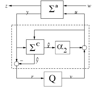
FIGURE 6.2
Parametrization of Nonlinear ${\mathcal{H}}_{\infty }$-Controllers with Measurement-Feedback; Adopted from IEEE Transactions on Automatic Control, vol. 40, no. 9, © 1995, “A state-space approach to parametrization of stabilizing controllers for nonlinear systems,” by Lu W.-M.

Theorem 6.1.4 Suppose all the hypotheses (i)-(iv) of Theorem 6.1.2 hold, and $k_{21}(x)k_{21}^T(x)=I$. In addition, assume the following hypothesis also holds:

(v) There exists an input-affine system ∑_Q as defined above, whose equilibrium-point q = 0 is locally asymptotically-stable, and is such that there exists a smooth positive-definite function U : N₄ → ℜ₊, locally defined in a neighborhood of q = 0 in $\mathcal{X}$ satisfying the HJE:

$U_q\left(q\right)a\left(q\right)+\frac{1}{2{\gamma }^2}{U}_q\left(q\right)b\left(q\right)b^T\left(q\right)U_q^T\left(q\right)+\frac{1}{2}{c}^T\left(q\right)c\left(q\right)=0.$

(6.29)

Then the family of controllers

${\displaystyle \sum {}_Q^c:}\{\begin{array}{l}\dot{\xi }=f^b\left(\xi \right)+G\left(y-h_2\left(\xi \right)\right)+\mathrm{\Gamma }\left(\xi \right)\upsilon \\ \dot{q}=a\left(q\right)+b\left(q\right)r\\ \upsilon =c\left(q\right)\\ r=y-\widehat{y}\\ u={\alpha }_2\left(\xi \right)+\upsilon \end{array}$

(6.30)

where

$f^b\left(\xi \right)=f\left(\xi \right)+g_1\left(\xi \right){\alpha }_1\left(\xi \right)+g_2\left(\xi \right){\alpha }_2\left(\xi \right),\widehat{y}={\tilde{h}}_2\left(\xi \right)=h_2\left(\xi \right)+k_{21}\left(\xi \right){\alpha }_1\left(\xi \right)$

solves the MFBNLHICP locally.

Proof: First observe that the controller (6.30) is exactly the controller given in (6.28) with explicit state-space realization for Σ^c. Thus, proving the result of this theorem also proves the result of Proposition 6.1.2.

Accordingly, we divide the proof into several steps:

(a) Consider the Hamiltonian function defined in Chapter 5:

$H\left(x,w,u\right)=V_x\left(x\right)\left(f\left(x\right)+g_1\left(x\right)w+g_2\left(x\right)u\right)+\frac{1}{2}\parallel h_1^T{\parallel }^2+\frac{1}{2}\parallel u{\parallel }^2-\frac{1}{2}{\gamma }^2\parallel w{\parallel }^2$

which is quadratic in (w, u). Observe that

${\left(\frac{\partial H}{\partial u}\right)}_{w={\alpha }_1\left(x\right)}=0,{\left(\frac{\partial H}{\partial u}\right)}_{u={\alpha }_2\left(x\right)}=0.$

Therefore for every (w, u) we have

$\begin{array}{l}{V}_x\left(x\right)\left(f\left(x\right)+g_1\left(x\right)w+g_2\left(x\right)u\right)=\frac{1}{2}[{\Vert u-{\alpha }_2\left(x\right)\Vert }^2-{\gamma }^2{\Vert w-{\alpha }_1\left(x\right)\Vert }^2-\\ {\Vert u\Vert }^2+{\gamma }^2{\Vert w\Vert }^2-{\Vert h_1\Vert }^2].\end{array}$

(b) Consider now the closed-loop system:

$\begin{array}{l}\dot{x}=f\left(x\right)+g_1\left(x\right)w+g_2\left(x\right)\left({\alpha }_2\left(\xi \right)+\upsilon \right)\\ \dot{\xi }=f^b\left(\xi \right)+G\left(\xi \right)\left(y-h_2\left(\xi \right)\right)+\mathrm{\Gamma }\left(\xi \right)\upsilon \end{array}\}$

(6.31)

and the augmented pseudo-Hamiltonian function

$\begin{array}{l}{H}^b\left(x,\xi ,\upsilon ,w,\lambda ,\mu \right)={\lambda }^T\left[f\left(x\right)+g_1\left(x\right)w+g_2\left(x\right)\left({\alpha }_2\left(\xi \right)+\upsilon \right)\right]+\\ {\mu }^T\left[f^b\left(\xi \right)+G\left(\xi \right)\left(y-h_2\left(\xi \right)\right)+\mathrm{\Gamma }\left(\xi \right)\upsilon \right]+\\ \frac{1}{2}\parallel {\alpha }_2\left(\xi \right)+\upsilon -{\alpha }_2\left(x\right){\parallel }^2-\frac{1}{2}{\gamma }^2\parallel w-{\alpha }_1\left(x\right){\parallel }^2.\end{array}$

By settings $(\tilde{v},\tilde{w})$ such that

${\left(\frac{\partial H^b}{\partial \upsilon }\right)}_{\upsilon =\tilde{\upsilon }}=0,{\left(\frac{\partial H^b}{\partial w}\right)}_{w=\tilde{w}}=0,$

then for every (v, w)we have

$H^b\left(x,\xi ,\upsilon ,w\right)=H_{\star }^b\left(x,\xi ,\upsilon ,w\right)+\frac{1}{2}{\Vert \upsilon -\tilde{\upsilon }\Vert }^2-\frac{1}{2}{\gamma }^2{\Vert w-\tilde{w}\Vert }^2,$

where

$H_{\star }^b\left(z,\xi ,\upsilon ,w\right)=H^b\left(x,\xi ,\tilde{\upsilon },\tilde{w},W_x^T,W_{\xi }^T\right)\le 0.$

Furthermore, along any trajectory of the closed-loop system (6.31),

$\begin{array}{l}\dot{W}=W_x\dot{x}+W_{\xi }\dot{\xi }=H_{\star }^b\left(x,\xi ,\upsilon ,w\right)+\frac{1}{2}{\Vert \upsilon -\tilde{\upsilon }\Vert }^2-\frac{1}{2}{\gamma }^2{\Vert w-\tilde{w}\Vert }^2-\\ \frac{1}{2}{\Vert {\alpha }_2\left(\xi \right)+\upsilon -{\alpha }_2\left(x\right)\Vert }^2-\frac{1}{2}{\gamma }^2{\Vert w-{\alpha }_1\left(x\right)\Vert }^2.\end{array}$

(c) Similarly, consider now the system (6.27). By hypothesis (v), we have

$U_q\left(q\right)\left(a\left(q\right)+b\left(q\right)r\right)=\frac{1}{2}\left[-{\gamma }^2{\Vert r-r^{\star }\Vert }^2-{\Vert \upsilon \Vert }^2+{\gamma }^2{\Vert r\Vert }^2\right]$

where $r^{*}=\frac{1}{{\gamma }^2}{b}^T\left(q\right)U_q^T\left(q\right).$

(d) Then, consider the Lyapunov-function candidate

$\mathrm{\Omega }\left(x,\xi ,q\right)=V\left(x\right)+W\left(x,\xi \right)+U\left(q\right),$

which is locally positive-definite by construction. Differentiating Ω along the trajectories of the closed-loop system (6.31), (6.27), we get

$\begin{array}{l}\dot{\mathrm{\Omega }}=V_x\left(x\right)\dot{x}+W_x\left(x,\xi \right)\dot{x}+W_{\xi }\left(x,\xi \right)\dot{\xi }+U_q\left(q\right)\dot{q}\\ =H_{\star }^b\left(x,\xi ,\upsilon ,w\right)+\frac{1}{2}\{[{\Vert u-{\alpha }_2\left(x\right)\Vert }^2-{\gamma }^2{\Vert w-{\alpha }_1\left(x\right)\Vert }^2-{\Vert u\Vert }^2+\\ {\gamma }^2{\Vert w\Vert }^2-{\Vert h_1\left(x\right)\Vert }^2+[{\Vert \upsilon -\tilde{\upsilon }\Vert }^2-{\gamma }^2{\Vert w-\tilde{w}\Vert }^2-{\Vert u-{\alpha }_2\left(x\right)\Vert }^2+\\ {\gamma }^2{\Vert w-{\alpha }_1\left(x\right)\Vert }^2]+\left[-{\gamma }^2{\Vert r-r^{\star }\Vert }^2-{\Vert \upsilon \Vert }^2+{\gamma }^2{\Vert r\Vert }^2\right]\}.\end{array}$

Notice that

${\Vert \upsilon -\tilde{\upsilon }\Vert }^2\le {\gamma }^2{\Vert r-r^{\star }\Vert }^2$

since ${\Vert Q\Vert }_{{\mathcal{H}}_{\infty }}\le \gamma$. Therefore

$\dot{\mathrm{\Omega }}\le \frac{1}{2}\left[{\gamma }^2{\Vert r\Vert }^2+{\Vert w\Vert }^2)-{\Vert \upsilon \Vert }^2-{\Vert z\Vert }^2\right].$

(6.32)

Integrating now the above inequality from t = t₀ to t = T, we have

$\mathrm{\Omega }\left(x\left(T\right),T\right)-\mathrm{\Omega }\left(x\left(t_0\right),t_0\right)\le \frac{1}{2}{\displaystyle {\int }_{t_0}^T\left[{\gamma }^2{\Vert r\Vert }^2+{\Vert w\Vert }^2-{\Vert \upsilon \Vert }^2-{\Vert z\Vert }^2\right]}dt.$

Which implies that the closed-loop system has ${\mathcal{L}}_2$-gain ≤ γ from $\left[\begin{array}{l}r\\ w\end{array}\right]$ as $\left[\begin{array}{l}v\\ z\end{array}\right]$ as desrired.

(e) To show closed-loop stability, set w = 0, r = 0, in (6.32) to get

$\dot{\mathrm{\Omega }}\le \text{\hspace{0.17em}-}\frac{1}{2}\left({\Vert z\Vert }^2+{\Vert \upsilon \Vert }^2\right).$

This proves that the equilibrium-point (x, ξ, q) = (0, 0, 0) is stable. Further, the condition that $\dot{\mathrm{\Omega }}=0$ implies that w = 0, r = 0, z = 0, v = 0 ⇒ u = 0, h₁(x) = 0, α₂(ξ) = 0.Thus, any trajectory of the system (x^o(t), ξ^o(t), q^o(t)) satisfying the above conditions, is necessarily a trajectory of the system

$\begin{array}{l}\dot{x}=f\left(x\right)\\ \dot{\xi }=f\left(\xi \right)+g_1\left(\xi \right){\alpha }_1\left(\xi \right)+G\left(\xi \right)\left(h_2\left(x\right)-h_2\left(\xi \right)\right)\\ \dot{q}=a\left(q\right).\end{array}$

Therefore, by Assumption (i) and the fact that $\dot{q}$ = a(q) is locally asymptotically-stable about q = 0, we have lim_t→∞(x(t), q(t)) = 0. Similarly, by Assumption (iii) and a well known stability property of cascade systems, we also have lim_t→∞ ξ(t) = 0. Finally, by LaSalle’s invariance-principle we conclude that the closed-loop system is locally asymptotically-stable. □

6.2    Output Measurement-Feedback Nonlinear ${\mathcal{H}}_{\infty }$ Tracking Control

In this section, we discuss the output measurement-feedback tracking problem which was discussed in Section 5.2 for the state-feedback problem. The objective is to design an output-feedback controller for the system (6.1) to track a reference signal which is generated as the output y_m of a reference model defined by

${\mathrm{\Sigma }}_{{}_m}:\{\begin{array}{l}\dot{x}=f_{m\left(x_m\right)},x_{m\left(t_0\right)}=x_{{}_{m0}}\\ y_m=h_m\left(x_m\right)\end{array}$

6.33

$x_m\in {\Re }^l,f_m:{\Re }^l\to {\Re }^l$. We assume also for simplicity that this system is completely observable (see References [268, 212]). The problem can then be defined as follows.

Definition 6.2.1 (Measurement-Feedback Nonlinear ${\mathcal{H}}_{\infty }$ (Suboptimal) Tracking Control Problem (MFBNLHITCP)). Find (if possible!) a dynamic output-feedback controller of the form

$\{\begin{array}{l}{\dot{x}}_c={\dot{\eta }}_c\left(x,x_m\right),x_c\left(t_0\right)=x_{c0}\\ u={\alpha }_{dyntrk}\left(x_c,x_m\right),{\alpha }_{dyntrk}:N_1\times {\tilde{N}}_m\to {\Re }^p\end{array}$

6.34

$x_c\subset {\Re }^n,N_c\subset \mathcal{X},{\tilde{N}}_m\subset {\Re }^l$, for some smooth function α_dyntrk, such that the closed-loop system (6.1), (6.34), (6.33) is exponentially stable about (x, x_c, x_m) = (0, 0, 0), and has for all initial conditions starting in $N_1\times {\tilde{N}}_m$ neighborhood of (0, 0), locally ${\mathcal{L}}_2$-gain from the disturbance signal w to the output z less than or equal to some prescribed number γ^⋆ > 0, as well as the tracking error satisfies lim_t→∞{y − y_m} = 0.

To solve the above problem, we consider the system (6.1) with

$z=\left[\begin{array}{l}{h}_1\left(x\right)\\ u\end{array}\right]$

and follow as in Section 5.2 a two-step design procedure.

$\underset{\_}{\text{Step}\text{1:}}$ We seek a feedforward dynamic-controller of the form

$\{\begin{array}{l}{\dot{x}}_c=a\left(x_c\right)+b\left(x_c\right)y\\ u=c\left(x_{c,}{x}_m\right)\end{array}$

6.35

where $x_c\in {\Re }^n$, so that the equilibrium point (x, x_c) = (0, 0) of the closed-loop system with w = 0,

$\begin{array}{l}\dot{x}=f\left(x\right)+g_2\left(x\right)c\left(x_{c,}{x}_m\right)\\ {\dot{x}}_c=a\left(x_c\right)+b\left(x_c\right)h_2\left(x\right)\end{array}$

is exponentially stable and there exists a neighborhood $\tilde{U}\subset \mathcal{X}\times {\Re }^n\times {\Re }^l$ of (0, 0, 0) such that, for all initial conditions $(x_0,x_{c0},x_{m0})\in \tilde{U}$, the solution (x(t), x_c(t), x_m(t)) of

$\{\begin{array}{l}\dot{x}=f\left(x\right)+g_2\left(x\right)c\left(x_{c,}{x}_m\right)\\ {\dot{x}}_c=a\left(x_c\right)+b\left(x_c\right)h_2\left(x\right)\\ {\dot{x}}_m=f_m\left(x_m\right)\end{array}$

satisfies

$\underset{t\to \infty }{\lim }{h}_1\left(\theta \left(x\left(t\right)\right)\right)-h_m\left(x_m\left(t\right)\right)=0.$

To solve this step, we similarly seek an invariant-manifold

${\tilde{M}}_{\theta ,\sigma }=\left\{x|x=\text{θ}\left(x_m\right),x_c=\sigma \left(x_m\right)\right\}$

which is invariant under the closed-loop dynamics (6.36) and is such that the error e = h₁(x(t)) − h_m(x_m(t)) vanishes identically on this submanifold. Again, this requires that the following necessary conditions are satisfied by the control law $u={\overline{u}}_{\star }(x_m)$:

$\begin{array}{l}\frac{\partial \theta }{\partial x_m}\left(x_m\right)f_m\left(x_m\right)=f\left(\theta \left(x_m\right)\right)+g_2\left(\theta \left(x_m\right){\overline{u}}_{\star }\left(x_m\right)\right)\\ \frac{\partial \sigma }{\partial x_m}\left(x_m\right)f\left(x_m\right)=a\left(\sigma \left(x_m\right)\right)+b\left(\sigma \left(x_m\right)\right)y_{\star }\left(x_m\right)\\ h_1\left(\theta \left(x\left(t\right)\right)\right)-h_m\left(x_m\left(t\right)\right)=0,\end{array}$

where ${\overline{u}}_{\star }(x_m)=c(\sigma (x_m),x_m),y_{\star }(x_m)=h_2(\theta (x_m))$.

Now, assuming the submanifold ${\tilde{M}}_{\theta ,\sigma }$ is found and the control law ${\overline{u}}_{\star }(x_m)$ has been designed to maintain the system on this submanifold, the next step is to design a feedback control v so as to drive the system onto the above submanifold and to achieve disturbance-attenuation and asymptotic-tracking. To formulate this step, we reconsider the combined system with the disturbances

$\{\begin{array}{l}\dot{x}=f\left(x\right)+g_1\left(x\right)w+g_2\left(x\right)u\\ \dot{x}=a\left(x_c\right)+b\left(x_c\right)h_2\left(x\right)+b\left(x_c\right)k_{21}\left(x\right)w\\ {\dot{x}}_m=f_m\left(x_m\right)\\ y=h_2\left(x\right)+k_{21}\left(x\right)w,\end{array}$

(6.36)

and introduce the following change of variables

$\begin{array}{l}{\xi }_1=x-\theta \left(x_m\right)\\ {\xi }_2=x_c-\sigma \left(x_m\right)\\ \upsilon =u-{\tilde{u}}_{\star }\left(x_m\right)\end{array}$

Then

$\begin{array}{l}{\dot{\xi }}_1={\tilde{F}}_1\left({\xi }_1,{\xi }_2,x_m\right)+\tilde{G}{}_{11}\left({\xi }_1,x_m\right)w+{\tilde{G}}_{12}\left({\xi }_1,x_m\right)\upsilon \\ {\dot{\xi }}_2=\tilde{F}\left({\xi }_1,{\xi }_2,x_m\right)+{\tilde{G}}_{21}\left({\xi }_2,x_m\right)w\\ {\dot{x}}_m=f_m\left(x_m\right)\\ y=\left[\begin{array}{l}{h}_2\left({\xi }_1{x}_m\right)+k_{21}\left({\xi }_1,x_m\right)w\\ h_m\left(x_m\right)\end{array}\right]\end{array}$

where

$\begin{array}{l}{\tilde{F}}_1\left({\xi }_1,x_m\right)=f\left({\xi }_1+\theta \left(x_m\right)\right)-\frac{\partial \theta }{\partial x_m}\left(x_m\right)f_m\left(x_m\right)+g_2\left({\xi }_1+\theta \left(x_m\right)\right){\overline{u}}_{\star }\left(x_m\right)\\ {\tilde{F}}_2\left({\xi }_2,x_m\right)=a\left({\xi }_2+\sigma \left(x_m\right)\right)+b\left({\xi }_2+\sigma \left(x_m\right)\right)h_2\left({\xi }_1+\theta \left(x_m\right)\right)-\frac{\partial \sigma }{\partial x_m}\left(x_m\right)f_m\left(x_m\right)\\ {\tilde{G}}_{11}\left({\xi }_1,x_m\right)=g_1\left({\xi }_1+\theta \left(x_m\right)\right)\\ {\tilde{G}}_{12}\left({\xi }_1,x_m\right)=g_2\left({\xi }_1+\theta \left(x_m\right)\right)\\ {\tilde{G}}_{21}\left({\xi }_2,x_m\right)=b\left({\xi }_2+\sigma \left(x_m\right)\right)k_{21}\left({\xi }_1+\theta \left(x_m\right)\right).\end{array}$

Similarly, we redefine the tracking error and the new penalty variable as

$\tilde{z}=\left[\begin{array}{l}{h}_1\left(\xi +\theta \left(x_m\right)\right)-h_m\left(x_m\right)\\ \upsilon \end{array}\right].$

$\underset{\_}{\text{Step}\text{2:}}$ Find a dynamic feedback compensator of the form (6.35) with an auxiliary output $v_{*}=v_{*}(\xi ,x_m)$ so that the closed-loop system (6.35), (6.36) is exponentially stable and along any trajectory (ξ(t), x_m(t)) of the closed-loop system, the ${\mathcal{L}}_2$-gain condition

$\begin{array}{l}{\displaystyle \underset{0}{\overset{T}{\int }}\left|\right|\tilde{z}\left(t\right)|{|}^2\le {\gamma }^2{\displaystyle \underset{0}{\overset{T}{\int }}\left|\right|w\left(t\right)|{|}^{2}dt+\tilde{\beta }\left(\xi \left(t_0\right),x_{m0}\right)}}\\ \iff {\displaystyle \underset{0}{\overset{T}{\int }}\left\{\left|\right|h_1\left(\xi +\theta \left(x_m\right)\right)-h_m\left(x_m\right)|{|}^2+|\left|\upsilon \right|{|}^2\right\}\le {\gamma }^2{\displaystyle \underset{0}{\overset{T}{\int }}\left|\right|w\left(t\right)|{|}^{2}dt+}}\beta \left(\xi \left(t_0\right),x_{m0}\right)\end{array}$

is satisfied for some function $\tilde{\beta }$, for all $w\in \mathcal{W}$, for all T < ∞ and all initial conditions (ξ₁(t₀), ξ₂(t₀), x_m0) in a sufficiently small neighborhood of the origin (0, 0).

The above problem is now a standard measurement-feedback ${\mathcal{H}}_{\infty }$ control problem, and can be solved using the techniques developed in the previous section.

6.3    Robust Output Measurement-Feedback Nonlinear ${\mathcal{H}}_{\infty }$-Control

In this section, we consider the robust output measurement-feedback nonlinear ${\mathcal{H}}_{\infty }$-control problem for the affine nonlinear system (6.1) in the presence of unmodelled dynamics and/or parameter variations. This problem has been considered in many references [34, 208, 223, 265, 284], and the set-up is shown in Figure 6.3. The approach presented here is based on [208]. For this purpose, the system is represented by the model:

${\displaystyle {\sum }_{△}^a:}\{\begin{array}{l}x=f\left(x\right)+\text{Δ}f\left(x,\theta ,t\right)+g_1\left(x\right)w+\left[g_2\left(x\right)+\text{Δ}{g}_2\left(x,\theta ,t\right)\right]u;\\ x\left(0\right)=x_0\\ z=h_1\left(x\right)=k_{12}\left(x\right)\text{u}\\ y=\left[h_2\left(x\right)+\text{Δ}{h}_2\left(x,\theta ,t\right)\right]+k_{21}\left(x\right)w\end{array}$

(6.37)

where all the variables and functions have their previous meanings and in addition $\mathcal{X}\to V^{\infty }(\mathcal{X}),\text{Δ}{g}_2:\mathcal{X}\to {\mathcal{M}}^{n\times p}(\mathcal{X})$, and $\text{Δ}{h}_2:\mathcal{X}\to {\Re }^m$ are unknown functions which belong to the set Ξ₁ of admissible uncertainties, and $\theta \in \mathrm{\Theta }\subset {\Re }^m$ are the system parameters which may vary over time within the set Θ.

Definition 6.3.1 (Robust Output Measurement-Feedback Nonlinear “_∞-Control Problem (RMFBNLHICP)). Find (if possible!) a dynamic controller of the form (6.3) such that the closed-loop system (6.37), (6.3) has locally ${\mathcal{L}}_2$-gain from the disturbance signal w to the output z less than or equal to some prescribed number γ^⋆ > 0 with internal stability, for all admissible uncertainties Δf, Δg₂, Δh₂, ∈ Ξ₁ and all parameter variations in Θ.

We begin by first characterizing the sets of admissible uncertainties of the system Ξ₁ and Θ₁ as

Assumption 6.3.1 The sets of admissible uncertainties of the system are characterized as for some known matrices H₁(.), F (., .), E₁(.), E₂(.), H₃(.), E₃ of appropriate dimensions.

$\begin{array}{l}{\text{Ξ}}_1=\{\text{Δ}f,\text{Δ}{g}_2,\text{Δ}{h}_2|\text{Δ}f\left(x,\theta ,t\right)=H_1\left(x\right)F\left(x,\theta ,t\right)E_1\left(x\right),\\ \text{Δ}{g}_2\left(x,\theta ,t\right)=g_2\left(x\right)F\left(x,\theta ,t\right)E_2\left(x\right),\text{Δ}{h}_2=H_3\left(x\right)F\left(x,\theta ,t\right)E_3\left(x\right),\left|\right|F\left(x,\theta ,t\right)|{|}^2\le 1,\\ \forall x\in \mathcal{X},\theta \in \mathrm{\Theta },t\in \Re \},\\ {\mathrm{\Theta }}_1=\left\{\theta |0\le {\theta }_u,|\left|\theta \right||\le \kappa <\infty \right\},\end{array}$

FIGURE 6.3
Configuration for Robust Nonlinear ${\mathcal{H}}_{\infty }$-Control with Measurement-Feedback

for some known matrices H₁(.), F (., .), E₁(.), E₂(.), H₃(.), E₃ of appropriate dimensions.

Then, to solve the RMFBNLHICP, we clearly only have to modify the solution to the nominal MFBNLHICP given in Theorems 6.1.1, 6.1.2, 6.1.3, and in particular, modify the HJIEs (inequalities) (6.39), (6.23), (5.12) to account for the uncertainties in Δf, Δg₂ and Δh₂.

The HJI-inequality (5.24) has already been modified in the form of the HJI-inequality (5.46) to obtain the solution to the RSFBNLHICP for all admissible uncertainties Δf, Δg₂ in Ξ. Therefore, it only remains to modify the HJI-inequality (6.23), or equation (6.16) to account for the uncertainties Δf, Δg₂, and Δh₂ in Ξ₁, Θ. If we choose to modify HJIE (6.16) to accomodate the uncertainties, then the result can be stated as a corollary to Theorem 6.1.3 as follows.

Corollary 6.3.1 Consider the nonlinear system (6.37) and assume that $k_{21}(x)k_{21}^T(x)=I$ in (6.2). Suppose also the following hold:

(i) The pair{f, h₁} is locally detectable.

(ii) There exists a smooth positive-definite function $\tilde{V}$ locally defined about the origin with $\tilde{V}(0)=0$ and satisfying the HJIE (5.46).

(iii) There exists an n × m matrix $G_{\text{Δ}}:\mathcal{X}\to {\mathcal{M}}^{n\times m}$ such that the equilibrium ξ = 0 of the system

$\dot{\xi }=f(\xi )+H_1(\xi )E_1(\xi )+g_1(\xi ){\alpha }_1(\xi )-G_{\text{Δ}}(\xi )(h_2(\xi )+H_3(\xi )E_3(\xi ))$

(6.38)

is locally asymptotically-stable.

(iv) There exists a smooth positive-semidefinite function $\tilde{W}\left(x,\xi \right)$ locally defined in a neighborhood ${\tilde{N}}_1\times {\tilde{N}}_1\subset \mathcal{X}\times \mathcal{X}$ of the origin (x, ξ) = (0, 0) such that $\tilde{W}(0,\xi )>0$ for each ξ ≠ 0, and satisfying the HJIE

$\begin{array}{l}\left[{\tilde{W}}_x\left(x,\xi \right)\tilde{W}\xi \left(x,\xi \right)\right]f_e\left(x,\xi \right)+\\ \frac{1}{2{\gamma }^2}\left[{\tilde{W}}_x\left(x,\xi \right){\tilde{W}}_{\xi }\left(x,\xi \right)\right]\left[\begin{array}{cc}{g}_1^T{g}_1^T\left(x\right)+H_1^T\left(x\right)H_1\left(x\right)& 0\\ 0& G\left(\xi \right)G^T\left(\xi \right){+}^0{H}_1^T\left(\xi \right)H_1\left(\xi \right)\end{array}\right]\times \\ \left[\begin{array}{l}{\tilde{W}}_x^T\left(x,\xi \right)\\ {\tilde{W}}_{\xi }^T\left(x,\xi \right)\end{array}\right]+\frac{1}{2{}^{\mathrm{}}}\left(h_e^T\left(x,\xi \right)h_e\left(x,\xi \right)+E_1^T\left(x\right)E_1\left(x\right)+E_3^T\left(\xi \right)E_3\left(\xi \right)\right)=0,\\ \tilde{W}\left(0,0\right)=0\left(x,\xi \right)\in {\tilde{N}}_1\times {\tilde{N}}_1,\end{array}$

(6.39)

where f_e(x, ξ), h_e(x, ξ) are as defined previously.

Then, the R MFBNLHICP for the system is solved by the output-feedback controller:

${\tilde{\mathrm{\Sigma }}}_2^c:\{\begin{array}{l}\dot{\xi }=f\left(\xi \right)+H_1\left(\xi \right)E_1\left(\xi \right)+g_1\left(\xi \right){\alpha }_1\left(\xi \right)+g_2\left(\xi \right){\alpha }_2\left(\xi \right)+G_{\text{Δ}}\left(\xi \right)[y-\\ h_2\left(\xi \right)-H_3\left(\xi \right)E_3\left(\xi \right)]\\ u={\alpha }_2\left(\xi \right),\end{array}$

(6.40)

Proof: The proof can be pursued along the same lines as Theorem 6.1.3. □

In the next section we discuss another aspect of robust control known as reliable control.

6.3.1    Reliable Robust Output-Feedback Nonlinear ${\mathcal{H}}_{\infty }$-Control

In this subsection, we discuss reliable control which is another aspect of robust control. The aim however in this case is to maintain control and stability in the event of a set of actuator or sensor failures. Failure detection is also another aspect of reliable control.

For the purpose of elucidating the scheme, let us represent the system on $\mathcal{X}\subset {\Re }^n$ in the form

${\mathrm{\Sigma }}^{ar}:\{\begin{array}{l}\dot{x}=f\left(x\right)+g_1\left(x\right)w_0+{\mathrm{\Sigma }}_{j=1}^p{g}_{\mathrm{2j}}\left(x\right)u_j;x\left(0\right)=x_0,\\ y_i=h_{2i}\left(x\right)+w_i,i=1,\mathrm{\dots },m,\\ z=\left[\begin{array}{l}{h}_1\left(x\right)\\ u_1\\ ⋮\\ u_p\end{array}\right],\end{array}$

(6.41)

where all the variables have their usual meanings and dimensions, and in addition $w={\left[\begin{array}{cccc}{w}_0^T& w_1^T& \dots & w_m^T\end{array}\right]}^T\in {\Re }^s$ is the overall disturbance input vector,

$\begin{array}{l}{g}_2\left(x\right)=\left[g_{21}\left(x\right)g_{22}\left(x\right)\mathrm{\dots }{g}_{2p}\left(x\right)\right],\\ h_2\left(x\right)={\left[h_{21}\left(x\right)h_{22}\left(x\right)\mathrm{\dots }{h}_{2m}\left(x\right)\right]}^T.\end{array}$

Without any loss of generality, we can also assume that f(0) = 0, h₁(0) = 0 and h_2i(0) = 0, i = 1, …, m. The problem is the following.

Definition 6.3.2 (Reliable Measurement-Feedback Nonlinear “_∞-Control Problem (RLMFBNLHICP)). Suppose Ƶ_a ⊂ {1, …, p} and Ƶ_s ⊂ {1, …, m} are the subsets of actuators and sensors respectively that are prone to failure. Find (if possible!) a dynamic controller of the form:

${\mathrm{\Sigma }}^{rc}:\{\begin{array}{l}\dot{\zeta }=a(\zeta )+b\left(\zeta \right)y\\ u=c\left(\zeta \right)\end{array}$

(6.42)

where $\zeta \in {\Re }^{\mathcal{V}}$, such that the closed-loop system denoted by Σ^ar ◦Σ^rc is locally asymptotically-stable and has locally ${\mathcal{L}}_2$-gain ≤ γ for all initial conditions in $N\subset \mathcal{X}$ and for all actuator and sensor failures in ${\mathcal{Z}}_a$ and ${\mathcal{Z}}_s$ respectively.

To solve the above problem, let $i_a\in {\mathcal{Z}}_a,{i^{\prime }}_a\in {\overline{\mathcal{Z}}}_a,j_s\in {\mathcal{Z}}_s,{j^{\prime }}_s\in {\overline{\mathcal{Z}}}_s$ denote the indices of the elements in ${\mathcal{Z}}_a,{\overline{\mathcal{Z}}}_a,{\mathcal{Z}}_s$ and ${\overline{\mathcal{Z}}}_s$ respectively, where the “bar” denotes “set complement.” Accordingly, introduce the following decomposition

$\begin{array}{l}{g}_2\left(x\right)=g_{2ia}\left(x\right)\oplus g_{2{i^{\prime }}_a}\left(x\right)\\ u=u_{ia}\oplus u_{i^{\prime }a}\\ h_2\left(x\right)=h_{2i_s}\left(x\right)\oplus h_{2{i^{\prime }}_s}\left(x\right)\\ y=y_{i_s}\oplus y_{i^{\prime }s}\\ w={\left[w_1\mathrm{\dots }{w}_m\right]}^T=w_{i_s}\oplus w_{{i^{\prime }}_s}\\ b\left(x\right)=\left[b_1\left(x\right)b_2\left(x\right)\mathrm{\dots }{b}_m\left(x\right)\right]=b_{i_s}\left(x\right)\oplus b_{{i^{\prime }}_s}\left(x\right)\end{array}$

where

$\begin{array}{l}{g}_{2i_a}\left(x\right)=\left[{\delta }_{ia}\left(1\right)g_{21}\left(x\right){\delta }_{ia}\left(2\right)g_{22}\left(x\right)\mathrm{\dots }{\delta }_{ia}\left(p\right)g_{2p}\left(x\right)\right]\\ u_{ia}\left(x\right)={\left[{\delta }_{ia}\left(1\right)u_1\left(x\right){\delta }_{ia}\left(2\right)u_2\left(x\right)\mathrm{\dots }{\delta }_{ia}\left(p\right)u_p\left(x\right)\right]}^T\\ h_{2i_s}\left(x\right)={\left[{\delta }_{is}\left(1\right)h_{21}\left(x\right){\delta }_{i_s}\left(2\right)h_{22}\left(x\right)\mathrm{\dots }{\delta }_{i_s}\left(m\right)h_{2m}\left(x\right)\right]}^T\\ y{i}_s\left(x\right)={\left[{\delta }_{i_s}\left(1\right)y_1{\delta }_{i_s}\left(2\right)y_2\mathrm{\dots }{\delta }_{i_s}\left(m\right)y_m\right]}^T\\ w_{i_s}\left(x\right)={\left[{\delta }_{i_s}\left(1\right)w_1{\delta }_{i_s}\left(2\right)w_2\mathrm{\dots }{\delta }_{i_s}\left(m\right)w_m\right]}^T\\ b_{i{}_s}\left(x\right)={\left[{\delta }_{i_s}\left(1\right)b_1\left(x\right){\delta }_{i_s}\left(2\right)b_2\left(x\right)\mathrm{\dots }{\delta }_{i_s}\left(m\right)b_m\left(x\right)\right]}^T\end{array}$

and

$\begin{array}{l}{\delta }_{i_a}\left(i\right)=\{\begin{array}{l}1ifi\in {\mathcal{Z}}_a\\ 0ifi\notin {\mathcal{Z}}_a\end{array}\\ \text{}\text{}\text{}\text{}\text{}\text{}\text{}\text{}\text{}\text{}\text{}\text{}\text{}\text{}\text{}\text{}\text{}\text{}{\delta }_{i_s}\left(j\right)=\{\begin{array}{l}1ifj\in {\mathcal{Z}}_s\\ 0ifj\notin {\mathcal{Z}}_s.\end{array}\end{array}$

Applying the controller Σ^rc to the system when actuator and/or sensor failures corresponding to the indices $i_a\in {\mathcal{Z}}_a$ and $i_s\in {\mathcal{Z}}_s$ occur, results in the closed-loop system ${\mathrm{\Sigma }}^{ar}\left({\mathcal{Z}}_s\right)\circ {\mathrm{\Sigma }}^{rs}\left({\mathcal{Z}}_a\right):$

$\{\begin{array}{l}\dot{x}=f(x)+g_1(x)w_0+g_{2i_a{}^{\prime }}(x)c_{{i^{\prime }}_a}(\zeta );x(0)=x_0\\ \dot{\zeta }=a(\zeta )+b_{{i^{\prime }}_s}(\zeta )y_{{i^{\prime }}_s}\\ =a(\zeta )+b_{{i^{\prime }}_s}(\zeta )h_{2i_s{}^{\prime }}(x)+b_{{i^{\prime }}_s}(\zeta )w_{{i^{\prime }}_s}\\ z_{{}_{{i^{\prime }}_a}}=\left[\begin{array}{l}{h}_1(x)\\ c_{{i^{\prime }}_a}(\zeta )\end{array}\right].\end{array}$

(6.43)

The aim now is to find the controller parameters a(.), b(.) and c(.), such that in the event of any actuator or sensor failure for any $i_a\in {\mathcal{Z}}_a$ and $i_s\in {\mathcal{Z}}_s$ respectively, the resulting closed-loop system above still has locally ${\mathcal{L}}_2$-gain ≤ γ from w_i'_s to z_i'_a and is locally asymptotically-stable. In this regard, define the Hamiltonian functions in the local coordinates (x, p) on $T^{\ast }\mathcal{X}$ by

$\begin{array}{l}{H}_s\left(x,p\right)=p^{T}f\left(x\right)+\frac{1}{2}{p}^T\left[\frac{1}{{\gamma }^2}{g}_1\left(x\right)g_1^T\left(x\right)-g_{2{\overline{\mathcal{Z}}}_a}\left(x\right)g_{2{\overline{\mathcal{Z}}}_a}^T\left(x\right)\right]p+\\ \frac{1}{2}{h}_1^T\left(x\right)h_1\left(x\right)+\frac{1}{2}{\gamma }^2{h}_{2\mathcal{Z}}^T\left(x\right)h_{2{\mathcal{Z}}_s}\left(x\right),\\ H_0\left(x,p\right)=p^{T}f\left(x\right)+\frac{1}{2{\gamma }^2}{p}^T{g}_1\left(x\right)g_1^T\left(x\right)p+\frac{1}{2}{p}^T{g}_{2{\mathcal{Z}}_a}\left(x\right)g_{2{\mathcal{Z}}_a}^T\left(x\right)p+\\ \frac{1}{2}{h}_1^T\left(x\right)h_1\left(x\right)-\frac{1}{2}{\gamma }^2{h}_{2{\tilde{\mathcal{Z}}}_s}^T\left(x\right)h_{2{\overline{\mathcal{Z}}}_s}\left(x\right).\end{array}$

Then, the following theorem gives a sufficient condition for the solvability of the reliable control problem.

Theorem 6.3.1 Consider the nonlinear system (6.41) and assume the following hold:

(i) The pair {f, h₁} is locally zero-state detectable.

(ii) There exists a smooth C² function ψ ≥ 0, ψ(0) = 0 and a C³ positive-definite function $\tilde{V}$ locally defined in a neighborhood N₀ of x = 0 with $\tilde{V}(0)=0$ and satisfying the HJIE:

$H_s\left(x,{\tilde{V}}_x^T\right)+\psi \left(x\right)=0.$

(6.44)

(iii) There exists a C³ positive-definite function $\tilde{U}$ locally defined in a neighborhood N₁ of x = 0 with $\tilde{U}(0)=0$ and satisfying the HJI-inequality:

$H_0\left(x,{\tilde{U}}_x^T\right)+\psi \left(x\right)\le 0,$

(6.45)

and such that $N_0\cap N_1\ne \cancel{0},H_0(x,{\tilde{U}}_x^T)+\psi (x)$ has nonsingular Hessian matrix at x = 0.

(iv) $\tilde{U}(x)-\tilde{V}(x)$ is positive definite, and there exists an n × m matrix function L(.) that satisfies the equation

$\left({\tilde{U}}_x-{\tilde{V}}_x\right)\left(x\right)L\left(x\right)={\gamma }^2{h}_2^T\left(x\right).$

(6.46)

Then, the controller Σ^rc solves the RLMFBNLHICP for the system Σ^ar with

$\begin{array}{l}a\left(\zeta \right)=f\left(\zeta \right)+\frac{1}{{\gamma }^2}{g}_1\left(\zeta \right)g_1^T\left(\zeta \right){\tilde{V}}_x^T\left(\zeta \right)-g_{2{\tilde{\mathcal{Z}}}_a}\left(\zeta \right)g_{2{\tilde{\mathcal{Z}}}_a}^T\left(\zeta \right){\tilde{V}}_x^T\left(\zeta \right)-L\left(\zeta \right)h_2\left(\zeta \right)\\ b\left(\zeta \right)=L\left(\zeta \right)\\ c\left(\zeta \right)=-g_2^T\left(\zeta \right){\tilde{V}}_x^T\left(\zeta \right).\end{array}$

Proof: The proof is lengthy, but can be found in Reference [285]. □

Remark 6.3.1 Theorem 6.3.1 provides a sufficient condition for the solvability of reliable controller design problem for the case of the primary contingency problem, where the set of sensors and actuators that are susceptible to failure is known a priori. Nevertheless by enlarging the sets ${\mathcal{Z}}_a,{\mathcal{Z}}_s$ to {1, …, p} and {1, …, m} respectively, the scheme can be extended to include all actuators and sensors.

We consider now an example.

Example 6.3.1 [285]. Consider the following second-order system.

$\left[\begin{array}{l}{\dot{x}}_1\\ {\dot{x}}_2\end{array}\right]=\left[\begin{array}{l}-2x_1+x_1{x}_2^2\\ x_2^3\end{array}\right]+\left[\begin{array}{l}1\\ x_1\end{array}\right]w_0+\left[\begin{array}{l}01\\ 11\end{array}\right]\left[\begin{array}{l}{u}_1\\ u_2\end{array}\right]$

(6.47)

$y=2x_1+2x_2+w_1$

(6.48)

$z={\left[x_1{x}_2^4{u}_1{u}_2\right]}^T.$

(6.49)

The index sets are given by ${\mathcal{Z}}_a=\left\{2\right\},{\mathcal{Z}}_s=\left\{\cancel{0}\right\}$, and the system is locally zero-state detectable. With γ = 0.81 and

$\psi \left(x\right)=\frac{1}{2}{x}_1^2+\frac{8{\gamma }^2}{{\gamma }^2-x_1^2}{x}_2^6,$

approximate solutions to the HJI-inequalities (6.44), (6.45) can be obtained as

$\tilde{V}\left(x\right)=0.4533x_1^2+0.3463x_1^2{x}_2^2+\frac{2{\gamma }^2}{{\gamma }^2-x_1^2}{x}_2^4$

(6.50)

$\tilde{U}\left(x\right)=1.5938x_1^2+0.3496x_1{x}_2+1.2667x_2^2$

(6.51)

respectively. Finally, equation (6.46) is solved to get

$L\left(x\right)={\left[1.01320.8961\right]}^T.$

The controller can then be realized by computing the values of a(x), b(x) and c(x) accordingly.