8

Nonlinear ${\mathcal{H}}_{\infty }$-Filtering

In this chapter, we discuss the nonlinear ${\mathcal{H}}_{\infty }$ sub-optimal filtering problem. This problem arises when the states of the system are not available for direct measurement, and so have to be estimated in some way, which in this case is to satisfy an ${\mathcal{H}}_{\infty }$-norm requirement. The states information may be required for feedback or other purposes, and the estimator is basically an observer [35] that uses the information on the measured output of the system and sometimes the input, to estimate the states.

It would be seen that the underlying structure of the ${\mathcal{H}}_{\infty }$ nonlinear filter is that of the Kalman-filter [35, 48, 119], but differs from it in the fact that (i) the plant is nonlinear; (ii) basic assumptions on the nature of the noise signal (which in the case of the Kalman-filter is Gaussian white noise); and (iii) the cost function to optimize. While the Kalman-filter [35] is a minimum-variance estimator, and is the best unbiased linear optimal filter [35, 48, 119], the ${\mathcal{H}}_{\infty }$ filter is derived from a completely deterministic setting, and is the optimal worst-case filter for all L₂-bounded noise signals.

The performance of the Kalman-filter for linear systems has been unmatched, and is still widely applied when the spectra of the noise signal is known. However, in the case when the statistics of the noise or disturbances are not known well, the Kalman-filter can only perform averagely. In addition, the nonlinear enhancement of the Kalman-filter or the “extended Kalman-filter” suffers from the usual problem with linearization, i.e., it can only perform well locally around a certain operating point for a nonlinear system, and under the same basic assumptions that the noise inputs are white.

It is therefore reasonable to expect that a filter that is inherently nonlinear and does not make any a priori assumptions on the spectra of the noise input, except that they have bounded energies, would perform better for a nonlinear system. Moreover, previous statistical nonlinear filtering techniques developed using minimum-variance [172] as well as maximum-likelihood [203] criteria are infinite-dimensional and too complicated to solve the filter differential equations. On the other hand, the nonlinear ${\mathcal{H}}_{\infty }$ filter is easy to derive, and relies on finding a smooth solution to a HJI-PDE which can be found using polynomial approximations.

The linear ${\mathcal{H}}_{\infty }$ filtering problem has been considered by many authors [207, 243, 281]. In [207], a fairly complete theory of linear ${\mathcal{H}}_{\infty }$ filtering and smoothing for finite and infinitehorizon problems is given. It is thus the purpose of this chapter to present the nonlinear counterparts of the filtering results. We begin with the continuous-time problem and then the discrete-time problem. Moreover, we also present results on the robust filtering problems.

8.1    Continuous-Time Nonlinear ${\mathcal{H}}_{\infty }$-Filtering

The general set-up for this problem is shown in Figure 8.1, where the plant is represented by an affine nonlinear system Σ^a, while F is the filter. The filter processes the measurement output y from the plant which is also corrupted by the noise signal w, and generates an estimate $\widehat{z}$ of the desired variable z. The plant can be represented by an affine causal state-space system defined on a smooth n-dimensional manifold $\mathcal{X}$ ⊆ ℜⁿ in coordinates x = (x₁,…, x_n) with zero-input:

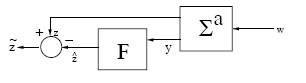
FIGURE 8.1
Configuration for Nonlinear ${\mathcal{H}}_{\infty }$-Filtering

${\sum }^a:\{\begin{array}{l}\dot{x}=f\left(x\right)+g_1\left(x\right)w;x\left(t_0\right)=x_0\\ z=h_1\left(x\right)\\ y=h_2\left(x\right)+k_{21}\left(x\right)w\end{array}$

(8.1)

where x ∈ $\mathcal{X}$ is the state vector, w ∈ W is an unknown disturbance (or noise) signal, which belongs to the set W ⊂ L₂([0, ∞), ℜ^r of admissible disturbances, the output y ∈ Y ⊂ ℜ^m is the measured output (or observation) of the system, and belongs to Y, the set of admissible outputs, and z ∈ ℜ^s is the output to be estimated.

The functions f : $\mathcal{X}$ → V ^∞($\mathcal{X}$), g₁ : $\mathcal{X}$ → M^n×r($\mathcal{X}$), h₁ : $\mathcal{X}$ → ℜ^s, h₂ : $\mathcal{X}$ → ℜ^m, and k₂₁ : $\mathcal{X}$ → M^m×r($\mathcal{X}$) are real C^∞ functions of x. Furthermore, we assume without any loss of generality that the system (8.1) has a unique equilibrium-point at x = 0 such that f(0) = 0, h₁(0) = h₂(0) = 0, and we also assume that there exists a unique solution x(t) for the system for all initial conditions x₀ and all w ∈ W.

The objective is to synthesize a causal filter, F, for estimating the state x(t) (or a function of it z = h₁(x)) from observations of y(τ) up to time t, over a time horizon [t₀, T ], i.e., from

${\text{Y}}_t\triangleq \left\{y\left(\tau \right):\tau \le t\right\},t\in \left[t_0,T\right],$

such that the L₂-gain from w to $\tilde{z}$ (the estimation error, to be defined later) is less than or equal to a given number γ > 0 for all w ∈ W, for all initial conditions in some subspace O ⊂ $\mathcal{X}$, i.e., we require that for a given γ > 0,

${\displaystyle {\int }_{t_0}^T{\Vert \tilde{z}\left(\tau \right)\Vert }^{2}d\tau }\le {\displaystyle {\int }_{t_0}^T{\Vert w\left(\tau \right)\Vert }^{2}d\tau ,T>t_0,}$

(8.2)

for all w ∈ W, and for all x₀ ∈ O. In addition, it is also required that with w ≡ 0, the penalty variable or estimation error satisfies $\underset{t\to \infty }{\lim }\tilde{z}\left(t\right)=0$

More formally, we define the local nonlinear ${\mathcal{H}}_{\infty }$ suboptimal filtering or state estimation problem as follows.

Definition 8.1.1 (Nonlinear ${\mathcal{H}}_{\infty }$ (Suboptimal) Filtering Problem (NLHIFP)). Given the plant Σ^a and a number γ^⋆ > 0. Find a causal filter $\mathcal{F}$ : $\mathcal{Y}$ → $\mathcal{X}$ which estimates x as $\widehat{x}$, such that

$\widehat{x}\left(t\right)=\mathcal{F}\left({\text{Y}}_t\right)$

and (8.2) is satisfied for all γ ≥ ${\gamma }^{\star }$, for all w ∈ W, and for all x₀ ∈ O. In addition, with w ≡ 0, we have $\underset{t\to \infty }{\lim }\tilde{z}\left(t\right)=0$

Moreover, if the above conditions are satisfied for all x(t₀) ∈ $\mathcal{X}$, we say that F solves the N L H I F P globally.

Remark 8.1.1 The problem defined above is the finite-horizon filtering problem. We have the infinite-horizon problem if we let T → ∞.

To solve the above problem, a structure is chosen for the filter $\mathcal{F}$. Based on our experience with linear systems, a “Kalman” structure is selected as:

$\begin{array}{l}\dot{\widehat{x}}=f\left(\widehat{x}\right)+L\left(\widehat{x},t\right)\left(y\left(t\right)-h_2\left(\widehat{x}\right)\right),\widehat{x}\left(t_0\right)={\widehat{x}}_0\\ \widehat{z}=h_1\left(\widehat{x}\right)\end{array}\}$

(8.3)

where $\widehat{x}$∈ $\mathcal{X}$ is the estimated state, L(., .) ∈ ℜ^n×m × ℜ is the error-gain matrix which has to be determined, and $\widehat{z}$ ∈ ℜ^s is the estimated output function. We can then define the output estimation error as

$\tilde{z}=z-\widehat{z}=h_1\left(x\right)-h_1\left(\widehat{x}\right),$

and the problem can be formulated as a two-person zero-sum differential game as discussed in Chapter 2. The cost functional is defined as

$\widehat{J}\left(w,L\right)\triangleq \frac{1}{2}{\displaystyle {\int }_{t_0}^T\left({\Vert z\left(t\right)\Vert }^2-{\text{γ}}^2{\Vert w\left(t\right)\Vert }^2\right)dt,}$

(8.4)

and we consider the problem of finding $L^{\star }$(.) such that Ĵ(w, L) is minimized subject to the dynamics (8.1), (8.3), for all w ∈ L₂[t₀, T], and for all x₀ ∈ $\mathcal{X}$. To proceed, we augment the system equations (8.1) and (8.3) into the following system:

$\{\begin{array}{l}{\dot{x}}^e=f^e\left(x^e\right)+g^e\left(x^e\right)w\\ \tilde{z}=h_1\left(x\right)-h_2\left(\widehat{x}\right)\end{array}$

(8.5)

where

$\begin{array}{l}{x}^e=\left(\begin{array}{l}x\\ \widehat{x}\end{array}\right),f^e{\left(x\right)}^e=\left(\begin{array}{l}f\left(x\right)\\ f\left(\widehat{x}\right)+L\left(\widehat{x}\right)\left(h_2\left(x\right)-h_2\left(x\right)\right)\end{array}\right),\\ g^e\left(x^e\right)=\left(\begin{array}{l}{g}_1\left(x\right)\\ L_1\left(\widehat{x}\right)k_{21}\left(x\right)\end{array}\right).\end{array}$

We then make the following assumption:

Assumption 8.1.1 The system matrices are such that

$\begin{array}{l}{k}_{21}\left(x\right)g_1^T\left(x\right)=0\\ k_{21}\left(x\right)k_{21}^T\left(x\right)=I\end{array}$

Remark 8.1.2 The first of the above assumptions means that the measurement-noise and the system-noise are independent; while the second is a normalization to simplify the problem.

To solve the above problem, we can apply the sufficient conditions given by Theorem 2.3.2 from Chapter 2, i.e., we consider the following HJIE:

$-Y_t\left(x^e,t\right)=\underset{L}{\inf }\underset{w}{\sup }\left\{Y_{x^e}\left(x^e,t\right)\left(f^e\left(x^e\right)+g^e\left(x^e\right)w\right)-\frac{1}{2}{\text{γ}}^2{w}^{T}w+\frac{1}{2}{z}^{T}z\right\},Y\left(x^e,T\right)=0$

(8.6)

for some smooth C¹ (with respect to both its arguments) function $Y:\widehat{N}\times \widehat{N}\times \Re \to \Re$ locally defined in a neighborhood $\widehat{N}$ of the origin x^e = 0. We then have the following lemma which is a restatement of Theorem 5.1.1.

Lemma 8.1.1 Suppose there exists a pair of strategies (w, L) = (w^⋆, L^⋆) for which there exists a positive-definite C¹ function $Y:\widehat{N}\times \widehat{N}\times \Re \to {\Re }_{+}$, locally defined in a neighborhood $\widehat{N}\times \widehat{N}\subset \mathcal{X}\times \mathcal{X}$ of x^e = 0 satisfying the HJIE (8.6). Then the pair (w^⋆, L^⋆) provides a saddle-point solution for the differential game.

To find the pair (w^⋆, L^⋆) that satisfies the HJIE, we proceed as in Chapter 5, by forming the Hamiltonian function Λ : T^⋆ ($\mathcal{X}$× $\mathcal{X}$) × $\mathcal{W}$ × $\mathcal{M}$^n×m → ℜ for the differential game:

$\Lambda \left(x^e,w,L,Y_{x^e}\right)=Y_{x^e}\left(x^e,t\right)\left(f^e\left(x^e\right)+g^e\left(x^e\right)w\right)-\frac{1}{2}{\text{γ}}^2{\Vert w\Vert }^2+\frac{1}{2}{\Vert z\Vert }^2.$

(8.7)

Then we apply the necessary conditions for the unconstrained optimization problem:

$\left(w^{\star },L^{\star }\right)=\text{arg}\left\{\underset{w}{\sup }\underset{L}{\min }\Lambda \left(x^e,w,L,Y_x\right)\right\}.$

We summarize the result in the following proposition.

Theorem 8.1.1 Consider the system (8.5), and suppose there exists a C¹(with respect to all its arguments) positive-definite function $Y:\widehat{N}\times \widehat{N}\times \Re \to {\Re }_{+}$ satisfying the HJIE:

$\begin{array}{l}{Y}_t\left(x^e,t\right)+Y_x\left(x^e,t\right)f\left(x\right)+Y_{\widehat{x}}\left(x^e,t\right)f\left(\widehat{x}\right)+\frac{1}{2{\text{γ}}^2}{Y}_x\left(x^e,t\right)g_1\left(x\right)g_1^T\left(x\right)Y_x^T\left(x^e,t\right)-\\ \text{}\text{}\text{}\frac{{\text{γ}}^2}{2}{\left(h_2\left(x\right)-h_2\left(\widehat{x}\right)\right)}^T\left(h_2\left(x\right)-h_2\left(\widehat{x}\right)\right)+\\ \frac{1}{2}{\left(h_1\left(x\right)-h_1\left(\widehat{x}\right)\right)}^T{\left(h_1\left(x\right)-h_1\left(\widehat{x}\right)\right)}^T=0,Y\left(x^e,T\right)=0,\end{array}$

(8.8)

together with the coupling condition

$Y_{\widehat{x}}\left(x^e,t\right)L\left(\widehat{x},t\right)=-{\text{γ}}^2{\left(h_2\left(x\right)-h_2\left(\widehat{x}\right)\right)}^T.$

(8.9)

Then the matrix $L(\widehat{x},t)$ satisfying (8.9) solves the finite horizon NLHIFP locally in $\widehat{N}$.

Proof: Consider the Hamiltonian function Λ(x^e, w, L, Y ^e_x). Since it is quadratic in w, we can apply the necessary condition for optimality, i.e.,

${\frac{\partial \Lambda }{\partial w}|}_{w=w^{\star }}=0$

to get

$w^{\star }:=\frac{1}{{\text{γ}}^2}\left(g_1^T\left(x\right)Y_x^T\left(x^e,t\right)+k_{21}^T\left(x\right)L^T\left(\widehat{x},t\right)Y_{\widehat{x}}^T\left(x^e,t\right)\right).$

Moreover, it can be checked that the Hessian matrix of Λ(x^e, w^⋆ , L, Y ^e_x) is negative-definite, and hence

$\Lambda \left(x^e,w^{\star },L,Y_x^e\right)\ge \Lambda \left(x^e,w^{},L,Y_x^e\right)\forall w\in \mathcal{W}.$

However, Λ is linear in L, so we cannot apply the above technique to obtain L^⋆. Instead, we use a completion of the squares method. Accordingly, substituting w^⋆ in (8.7), we get

$\begin{array}{l}\Lambda \left(x^e,w^{\star },L,Y_x^e\right)=\left(Y_x\left(x^e,t\right)f\left(x\right)+Y_{\widehat{x}}\left(x^e,t\right)f\left(\widehat{x}\right)\right)+Y_{\widehat{x}}\left(x^e,t\right)L\left(\widehat{x},t\right)\left(h_2\left(x\right)-h_2\left(\widehat{x}\right)\right)+\\ \frac{1}{2{\text{γ}}^2}{Y}_x\left(x^e,t\right)g_1\left(x\right)g_1^T\left(x\right)Y_x^T\left(x^e,t\right)+\frac{1}{2}{z}^{T}z+\\ \frac{1}{2{\text{γ}}^2}{Y}_{\widehat{x}}\left(x^e,t\right)L\left(\widehat{x},t\right)\left(x\right)L^T\left(\widehat{x},t\right)Y_{\widehat{x}}^T\left(x^e,t\right).\end{array}$

Now, completing the squares for L in the above expression, we get

$\begin{array}{l}\Lambda \left(x^e,w^{\star },L,Y_x^e\right)=Y_x\left(x^e,t\right)f\left(x\right)+Y_{\widehat{x}}\left(x^e,t\right)f\left(\widehat{x}\right)-\frac{1}{2}{\text{γ}}^2{\Vert \left(h_2\left(x\right)-h_2\left(\widehat{x}\right)\right)\Vert }^2+\\ \frac{1}{2{\text{γ}}^2}{\Vert L^T\left(\widehat{x},t\right)Y_{\widehat{x}}^T\left(x^e,t\right)+{\text{γ}}^2\left(h_2\left(x\right)-h_2\left(\widehat{x}\right)\right)\Vert }^2+\frac{1}{2}{z}^{T}z+\\ \frac{1}{2{\text{γ}}^2}{Y}_x\left(x^e,t\right)g_1\left(x\right)g_1^T\left(x\right)Y_x^T\left(x^e,t\right).\end{array}$

Thus, taking L^⋆ as in (8.9) renders the saddle-point conditions

$\Lambda \left(w,L^{\star }\right)\le \Lambda \left(w^{\star },L^{\star }\right)\le \left(w^{\star },L\right)$

satisfied for all (w, L) ∈ W × ℜ^n×m × ℜ, and the HJIE (8.6) reduces to (8.8). By Lemma 8.1.1, we conclude that (w^⋆ , L^⋆ ) is indeed a saddle-point solution for the game. Finally, it is very easy to show from the HJIE (8.8) that the L₂-gain condition (8.2) is also satisfied. □

Remark 8.1.3 By virtue of the side-condition (8.9), the HJIE (8.8) can be represented as

$\begin{array}{l}{Y}_t\left(x^e,t\right)+Y_x\left(x^e,t\right)f\left(x\right)+Y_{\widehat{x}}\left(x^e,t\right)f\left(\widehat{x}\right)+\frac{1}{2{\text{γ}}^2}{Y}_x\left(x^e,t\right)g_1\left(x\right)g_1^T\left(x\right)Y_x^T\left(x^e,t\right)\\ -\frac{1}{2{\text{γ}}^2}{Y}_x\left(x^e,t\right)L\left(\widehat{x},t\right)\left(x\right)L^T\left(\widehat{x},t\right)Y_{\widehat{x}}^T\left(x^e,t\right)+\frac{1}{2}{\left(h_1\left(x\right)-h_1\left(\widehat{x}\right)\right)}^T\left(h_1\left(x\right)-h_1\left(\widehat{x}\right)\right)=0,\\ Y\left(x^e,T\right)=0,\end{array}$

(8.10)

Remark 8.1.4 The above result, Theorem 8.1.1, can also be obtained from a dissipative systems perspective. Indeed, it can be checked that a function Y (., .) satisfying the HJIE (8.8) renders the dissipation-inequality

$Y\left(x^e\left(T\right),T\right)-Y\left(x^e\left(t_0\right),t_0\right)\le \frac{1}{2}{\displaystyle {\int }_{t_0}^T\left({\text{γ}}^2{\Vert w\left(t\right)\Vert }^2-{\Vert \tilde{z}\left(t\right)\Vert }^2\right)dt}$

(8.11)

satisfied for all x^e(t₀) and all w ∈ W. Conversely, it can also be shown (as it has been shown in the previous chapters), that a function Y (., .) satisfying the dissipation-inequality (8.11) also satisfies in more general terms the HJI-inequality (8.8) with “=” replaced by “≤”. Thus, this observation allows us to solve a HJI-inequality which is substantially easier and more advantageous to solve.

For the case of the LTI system

${\sum }^l:\{\begin{array}{l}\dot{x}=Ax+B_{1}w,x\left(t_0\right)=x_0\\ \tilde{z}=C_1\left(x-\widehat{x}\right)\\ y=C_{2}x+D_{21}w,\end{array}$

(8.12)

we have the following corollary.

Corollary 8.1.1 Consider the LTI system Σ^l (8.12) and the filtering problem for this system. Suppose there exists a symmetric positive-definite solution P to the Riccati-ODE:

$\dot{P}\left(t\right)=A^{T}P\left(t\right)+P\left(t\right)A+P\left(t\right)\left[\frac{1}{{\gamma }^2}{C}_1^T{C}_1-C_2^T{C}_2\right]P\left(t\right)+B_1{B}_1^T,p\left(T\right)=0.$

(8.13)

Then, the filter

$\dot{\widehat{x}}=A\widehat{x}+L\left(t\right)\left(y-C_2\widehat{x}\right)$

solves the finite-horizon linear ℋ_∞ filtering problem if the gain-matrix L(t) is taken as

$L\left(t\right)=P\left(t\right)C_2^T.$

Proof: Assume D₂₁D^T₂₁ = I, D₂₁B₁ = 0, t₀ = 0. Let P (t₀) > 0, and consider the positive-definite function

$Y\left(x,\widehat{x},t\right)=\frac{1}{2}{\text{γ}}^2{\left(x-\widehat{x}\right)}^T{P}^{-1}\left(t\right)\left(x-\widehat{x}\right),P\left(t\right)>0.$

(8.14)

Taking partial-derivatives and substituting in (8.8), we obtain

$\begin{array}{l}-\frac{1}{2}{\text{γ}}^2{\left(x-\widehat{x}\right)}^T{P}^{-1}\left(t\right)\dot{P}\left(t\right)P^{-1}\left(x-\widehat{x}\right)+{\text{γ}}^2{\left(x-\widehat{x}\right)}^T{P}^{-1}\left(t\right)A\left(x-\widehat{x}\right)+\\ \frac{{\text{γ}}^2}{2}{\left(x-\widehat{x}\right)}^T{P}^{-1}\left(t\right)B_1{B}_1^T{P}^{-1}\left(t\right)\left(x-\widehat{x}\right)-\frac{{\text{γ}}^2}{2}{\left(x-\widehat{x}\right)}^T{C}_1^T{C}_2\left(x-\widehat{x}\right)+\\ \frac{1}{2}{\left(x-\widehat{x}\right)}^T{C}_1^T{C}_1\left(x-\widehat{x}\right)=0.\end{array}$

(8.15)

Splitting the second term in the left-hand-side into two (since it is a scalar):

$\begin{array}{l}{\text{γ}}^2{\left(x-\widehat{x}\right)}^T{P}^{-1}\left(t\right)A\left(x-\widehat{x}\right)=\frac{1}{2}{\text{γ}}^2{\left(x-\widehat{x}\right)}^T{P}^{-1}\left(t\right)A\left(x-\widehat{x}\right)+\\ \frac{1}{2}{\text{γ}}^2{\left(x-\widehat{x}\right)}^T{P}^{-1}\left(t\right)A\left(x-\widehat{x}\right),\end{array}$

and substituting in the above equation, we get upon cancellation,

$\begin{array}{l}{P}^{-1}\left(t\right)\dot{P}\left(t\right)P^{-1}\left(t\right)=P^{-1}\left(t\right)A+A^T{P}^{-1}\left(t\right)+P^{-1}\left(t\right)B_1{B}_1^T{P}^{-1}\left(t\right)-\\ C_2^T{C}_2+{\text{γ}}^{-2}{C}_1^T{C}_1.\end{array}$

(8.16)

Finally, multiplying the above equation from the left and from the right by P (t), we get the Riccati ODE (8.13). The terminal condition is obtained by setting t = T in (8.14) and equating to zero.

Furthermore, substituting in (8.9) we get after cancellation

$P^{-1}\left(t\right)L\left(t\right)=C_2^T\text{or}\text{L}\left(t\right)=P\left(t\right)C_2^T.\square$

Remark 8.1.5 Note that, if we used the HJIE (8.10) instead, or by substituting C₂ = P ⁻¹(t)L(t) in (8.16), we get the following Riccati ODE after simplification:

$\dot{P}\left(t\right)=A^{T}P\left(t\right)+P\left(t\right)A+P\left(t\right)\left[\frac{1}{{\text{γ}}^2}{C}_1^T{C}_1-L^T\left(t\right)L\left(t\right)\right]p\left(t\right)+B_1{B}_1^T,P\left(T\right)=0$

This result is the same as in reference [207]. In addition, cancelling (x− $\widehat{x}$) from (8.15), and then multipling both sides by P (t), followed by the factorization, will result in the following alternative filter Riccati ODE

$\dot{P}\left(t\right)=P\left(t\right)A^T+AP\left(t\right)+P\left(t\right)\left[\frac{1}{{\text{γ}}^2}{C}_1^T{C}_1-C_2^T{C}_2\right]p\left(t\right)+B_1{B}_1^T,P\left(T\right)=0.$

(8.17)

8.1.1    Infinite-Horizon Continuous-Time Nonlinear ${\mathcal{H}}_{\infty }$-Filtering

In this subsection, we discuss the infinite-horizon filter in which case we let T → ∞. Since we are interested in finding time-invariant gains for the filter, we seek a time-independent function: $Y:{\widehat{N}}_1\times {\widehat{N}}_1\to {\Re }_{+}$ such that the HJIE:

$\begin{array}{l}{Y}_x\left(x^e\right)f\left(x\right)+Y_{\widehat{x}}\left(x^e\right)f\left(\widehat{x}\right)+\frac{1}{2{\text{γ}}^2}{Y}_x\left(x^e,t\right)g_1\left(x\right)g_1^T\left(x\right)Y_x^T\left(x^e\right)-\\ \frac{{\text{γ}}^2}{2}{\left(h_2\left(x\right)-h_2\left(\widehat{x}\right)\right)}^T\left(h_2\left(x\right)-h_2\left(\widehat{x}\right)\right)+\\ \frac{1}{2}{\left(h_1\left(x\right)-h_1\left(\widehat{x}\right)\right)}^T\left(h_1\left(x\right)-h_1\left(\widehat{x}\right)\right)=0,Y\left(0\right)=0,x,\widehat{x}\in {\widehat{N}}_1\end{array}$

(8.18)

is satisfied, together with the coupling condition

$Y_{\widehat{x}}\left(x^e\right)L\left(\widehat{x}\right)=-{\text{γ}}^2{\left(h_2\left(x\right)-h_2\left(\widehat{x}\right)\right)}^{T}x,\widehat{x}\in {\widehat{N}}_1.$

(8.19)

Or equivalently, the HJIE:

$\begin{array}{l}{Y}_x\left(x^e\right)f\left(x\right)+Y_{\widehat{x}}\left(x^e\right)f\left(\widehat{x}\right)+\frac{1}{2{\text{γ}}^2}{Y}_x\left(x^e\right)g_1\left(x\right)g_1^T\left(x\right)Y_x^T\left(x^e\right)-\\ \frac{1}{2{\text{γ}}^2}{Y}_x\left(x^e\right)L\left(\widehat{x}\right)\left(x\right)L^T\left(\widehat{x}\right)Y_{\widehat{x}}^T\left(x^e\right)+\\ \frac{1}{2}{\left(h_1\left(x\right)-h_1\left(\widehat{x}\right)\right)}^T\left(h_1\left(x\right)-h_1\left(\widehat{x}\right)\right)=0,Y\left(0\right)=0,x,\widehat{x}\in {\widehat{N}}_1\end{array}$

(8.20)

However here, since the estimation is carried over an infinite-horizon, it is necessary to ensure that the interconnected system (8.5) is stable with w = 0. This will in turn guarantee that we can find a smooth function Y(.) which satisfies the HJIE (8.18) and provides an optimal gain for the filter. One additional assumption is however required: the system (8.1) must be locally asymptotically-stable. The following theorem summarizes this development.

Proposition 8.1.1 Consider the nonlinear system (8.1) and the infinite-horizon N L H I F P for it. Suppose the system is locally asymptotically-stable, and there exists a C¹-positive-definite function $Y:{\widehat{N}}_1\times {\widehat{N}}_1\to {\Re }_{+}$ locally defined in a neighborhood of (x, $\widehat{x}$) = (0, 0) and satisfying the HJIE (8.18) together with the coupling condition (8.19), or equivalently the HJIE (8.20) for some matrix function L(.) ∈ $\mathcal{M}$^n×m. Then, the infinite-horizon N L H I F P is locally solvable in ${\widehat{N}}_1$ and the interconnected system is locally asymptotically-stable.

Proof: By Remark 8.1.4, any function Y satisfying (8.18)-(8.19) or (8.20) also satisfies the dissipation-inequality

$Y\left(x^e\left(t\right)\right)-Y\left(x^e\left(t_0\right)\right)\le \frac{1}{2}{\displaystyle {\int }_{t_0}^t\left({\text{γ}}^2{\Vert w\left(t\right)\Vert }^2-{\Vert \tilde{z}\left(t\right)\Vert }^2\right)dt}$

(8.21)

for all t and all w ∈ W. Differentiating this inequality along the trajectories of the interconnected system with w = 0, we get

$\dot{Y}\left(x^e\left(t\right)\right)=-\frac{1}{2}{\Vert z\Vert }^2.$

Thus, the interconnected system is stable. In addition, any trajectory x^e(t) of the system starting in ${\widehat{N}}_1$ neighborhood of the origin x^e = 0 such that $\dot{Y}(t)\equiv 0\forall t\ge t_s$, is such that h₁(x(t)) = h₁($\widehat{x}$(t)) and x(t) = $\widehat{x}$(t) ∀t ≥ t_s. This further implies that h₂(x(t)) = h₂($\widehat{x}$(t)), and therefore, it must be a trajectory of the free-system

${\dot{x}}^e=f\left(x\right)\text{=}\left(\begin{array}{l}f\left(x\right)\\ f\left(\widehat{x}\right)\end{array}\right).$

By local asymptotic-stability of the free-system $\dot{x}=f(x)$, we have local asymptotic-stability of the interconnected system. □

Remark 8.1.6 Note that, in the above proposition, it is not necessary to have a stable system for ${\mathcal{H}}_{\infty }$ estimation. However, estimating the states of an unstable system is of no practical benefit.

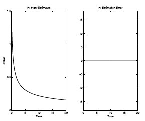
FIGURE 8.2
Nonlinear ${\mathcal{H}}_{\infty }$-Filter Performance with Known Initial Condition

Example 8.1.1 Consider a simple scalar example

$\begin{array}{l}\dot{x}=-x^3\\ y=x+w\\ \widehat{z}=x-\widehat{x}.\end{array}$

We consider the infinite-horizon problem and the HJIE (8.18) together with (8.19). Substituting in these equations we get

$\begin{array}{l}-x^3{Y}_x-x^3{Y}_{\widehat{x}}-\frac{{\text{γ}}^2}{2}{\left(x-\widehat{x}\right)}^2+\frac{1}{2}{\left(x-\widehat{x}\right)}^2=0,Y\left(0,0\right)=0\\ Y_{\widehat{x}}{l}_{\infty }=-2{\text{γ}}^2\left(x-\widehat{x}\right).\end{array}$

If we let γ = 1, then

$-x^3{Y}_x-\widehat{x}{Y}_{\widehat{x}}=0$

and it can be checked that

$Y_x=x,Y_{\widehat{x}}=\widehat{x}$

solve the HJI-inequality, and result in

$Y=\left(x,\widehat{x}\right)=\frac{1}{2}\left(x^2+{\widehat{x}}^2\right)\Rightarrow l_{\infty }^{\star }=\frac{-2\left(x-\widehat{x}\right)}{\widehat{x}}.$

The results of simulation of the system with this filter are shown on Figures 8.2 and 8.3. A noise signal

$w\left(t\right)=w_0+0.1\sin \left(t\right)$

where w₀ is a zero-mean Gaussian white-noise with unit variance, is also added to the output.

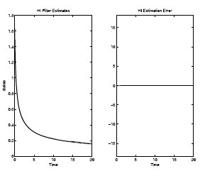
FIGURE 8.3
Nonlinear ${\mathcal{H}}_{\infty }$-Filter Performance with Unknown Initial Condition

8.1.2    The Linearized Filter

Because of the difficulty of solving the HJIE in implementation issues, it is sometimes useful to consider the linearized filter and solve the associated Riccati equation. Such a filter will be a variant of the extended-Kalman filter, but is different from it in the sense that, in the extended-Kalman filter, the finite-horizon Riccati equation is solved at every instant, while for this filter, we solve an infinite-horizon Riccati equation. Accordingly, let

$F=\frac{\partial f}{\partial x}\left(0\right),G_1=g_1(0),H_1=\frac{\partial h_1}{\partial x}\left(0\right),H_2=\frac{\partial h_2}{\partial x}\left(0\right)$

(8.22)

be a linearization of the system about x = 0. Then the following result follows trivially.

Proposition 8.1.2 Consider the nonlinear system (8.1) and its linearization (8.22). Suppose for some γ > 0 there exists a real positive-definite symmetric solution to the filter algebraic-Riccati equation (FARE):

$P{F}^T+FP+P\left[\frac{1}{{\text{γ}}^2}{H}_1^T{H}_1-H_2^T{H}_2\right]P+G_1{G}_1^T=0,$

(8.23)

or

$P{F}^T+FP+P\left[\frac{1}{{\text{γ}}^2}{H}_1^T{H}_1-L^{T}L\right]P+G_1{G}_1^T=0,$

(8.24)

for some matrix ${\mathrm{L = PH}}_2^T$. Then, the filter

$\dot{\widehat{x}}=F\widehat{x}+L\left(y-H_2\widehat{x}\right)$

solves the infinite-horizon N L H I F P for the system (8.1) locally on a small neighborhood O of x = 0 if the gain matrix L is taken as specified above.

Proof: Proof follows trivially from linearization. It can be checked that the function $V(x)=\frac{1}{2}{\gamma }^2(x-\widehat{x})P^{-1}(x-\widehat{x})$, P a solution of (8.23) or (8.24) satisfies the HJIE (8.8) together with (8.9) or equivalently the HJIE (8.10) for the linearized system.

Remark 8.1.7 To guarantee that there exists a positive-definite solution to the ARE (8.23) or (8.24), it is necessary for the linearized system (8.22) or [F, H₁] to be detectable (see [292]).

8.2    Continuous-Time Robust Nonlinear ${\mathcal{H}}_{\infty }$-Filtering

In this section we discuss the continuous-time robust nonlinear ${\mathcal{H}}_{\infty }$-filtering problem (R N L H I F) in the presence of structured uncertainties in the system. This situation is shown in Figure 8.4 below, and arises when the system model is not known exactly, as is usually the case in practice. For this purpose, we consider the following model of the system with uncertainties:

${\sum }^{a,\mathrm{\Delta }}:\{\begin{array}{l}\dot{x}=f\left(x\right)+\mathrm{\Delta }f\left(x,t\right)+g_1\left(x\right)w;x\left(0\right)=0\\ z=h_1\left(x\right)\\ y=h_2\left(x\right)+\mathrm{\Delta }{h}_2\left(x,t\right)+k_{21}\left(x\right)w\end{array}$

(8.25)

where all the variables have their previous meanings. In addition, Δf : X × ℜ → V ^∞X, Δf(0, t) = 0, Δh₂ : X × ℜ → ℜ^m, Δh₂(0, t) = 0 are the uncertainties of the system which belong to the set of admissible uncertainties Ξ_Δ and is defined as follows.

Assumption 8.2.1 The admissible uncertainties of the system are structured and matched, and they belong to the following set:

$\begin{array}{l}{\Xi }_{\mathrm{\Delta }}=\{\mathrm{\Delta }f,\mathrm{\Delta }{h}_2|\mathrm{\Delta }f\left(x,t\right)=H_1\left(x\right)F\left(x,t\right)E\left(x\right),\mathrm{\Delta }{h}_2\left(x,t\right)=H_2\left(x\right)F\left(x,t\right)E\left(x\right),\\ E\left(0\right)=0,{\displaystyle {\int }_0^{\infty }\left({\Vert E\left(x\right)\Vert }^2-{\Vert F\left(x,t\right)E\left(x\right)\Vert }^2\right)dt\ge 0,and}\\ \left[k_{21}\left(x\right)H_2\left(x\right)\right]{\left[k_{21}\left(x\right)H_2\left(x\right)\right]}^T>0\forall x\in \mathcal{X},t\in \Re \}\end{array}$

where H₁(.), H₂(.), F (., .), E(.) have appropriate dimensions.

The problem is the following.

Definition 8.2.1 (Robust Nonlinear ${\mathcal{H}}_{\infty }$-Filtering Problem (RNLHIFP)). Find a filter of the form

${\sum }^f:\{\begin{array}{l}\dot{\xi }=a\left(\xi \right)+b\left(\xi \right)y,\xi \left(0\right)=0\\ \widehat{z}=c\left(\xi \right)\end{array}$

(8.26)

where ξ ∈ $\mathcal{X}$ is the state estimate, y ∈ ℜ^m is the system output, $\widehat{z}$ is the estimated variable, and the functions a : $\mathcal{X}$ → V ^∞$\mathcal{X}$, a(0) = 0, b : $\mathcal{X}$ → M^n×m, c : $\mathcal{X}$ → ℜ^s, c(0) = 0 are smooth C² functions, such that the L₂-gain from w to the estimation error $\tilde{z}=z-\widehat{z}$ is less than or equal to a given number γ > 0, i.e.,

${\displaystyle {\int }_0^T{\Vert \tilde{z}\Vert }^{2}dt\le {\text{γ}}^2{\displaystyle {\int }_0^T{\Vert w\left(t\right)\Vert }^{2}dt}}$

(8.27)

for all T > 0, all w ∈ $\mathcal{L}$₂[0, T ], and all admissible uncertainties. In addition with w ≡ 0, we have lim_t→∞ $\tilde{z}$(t) = 0.

To solve the above problem, we first recall the following result [210] which gives sufficient conditions for the solvability of the N L H I F P for the nominal system (i.e., without the uncertainties Δf(x, t) and Δh₂(x, t)). Without any loss of generality, we shall also assume for the remainder of this section that $\underset{\_}{\text{γ}=1}$ henceforth.

Theorem 8.2.1 Consider the nominal system (8.25) without the uncertainties Δf(x, t) and Δh₂(x, t) and the N L H I F P for this system. Suppose there exists a positive-semidefinite function $\psi :\tilde{N}\times \tilde{N}\to \Re$ locally defined in a neighborhood $\tilde{N}\times \tilde{N}$ of the origin (x, ξ) = 0 such that the following HJIE is satisfied

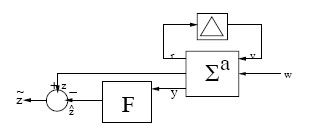
FIGURE 8.4
Configuration for Robust Nonlinear ${\mathcal{H}}_{\infty }$-Filtering

$HJI\left(x,\xi \right)+{\tilde{b}}^T\left(x,\xi \right)R\left(x\right)\tilde{b}\left(x,\xi \right)\le 0$

(8.28)

for all x, ξ ∈ $\tilde{N}\times \tilde{N}$, where

$\begin{array}{l}HJI\left(x,\xi \right)\triangleq \left[{\text{ψ}}_x\left(x,\xi \right){\text{ψ}}_{\xi }\left(x,\xi \right)\right]\left[\tilde{f}\left(x,\xi \right)+\tilde{g}\left(x,\xi \right){\Psi }_x^T\left(\xi ,\xi \right)\right]+\\ \frac{1}{4}\left[{\Psi }_x\left(x,\xi \right){\Psi }_{\xi }\left(x,\xi \right)\right]\tilde{k}\left(x,\xi \right){\tilde{k}}^T\left(x,\xi \right)\left[\begin{array}{l}{\Psi }_x^T\left(x,\xi \right)\\ {\Psi }_{\xi }^T\left(x,\xi \right)\end{array}\right]-\\ \frac{1}{4}{\Psi }_x\left(\xi ,\xi \right)g_1\left(\xi \right)k_{21}^T\left(\xi \right)R^{-1}\left(x\right)k_{21}\left(\xi \right)g_1^T\left(\xi \right){\Psi }_x^T\left(\xi ,\xi \right)-\\ {\tilde{h}}_2\left(x,\xi \right)R^{-1}\left(x\right){\tilde{h}}_2\left(x,\xi \right)+{\tilde{h}}_1^T\left(x,\xi \right){\tilde{h}}_1\left(x,\xi \right)+\\ \frac{1}{2}{\Psi }_x\left(\xi ,\xi \right)g_1\left(\xi \right)k_{21}^T\left(\xi \right)R^{-1}\left(x\right){\tilde{h}}_2\left(x,\xi \right)\\ \tilde{b}\left(x,\xi \right)=\frac{1}{2}{b}^T\left(\xi \right){\Psi }_{\xi }^T\left(x,\xi \right)+R^{-1}\left(x\right)\left[\frac{1}{2}{k}_{21}\left(x\right)g_1^T\left(x\right){\Psi }_x^T\left(x,\xi \right)+{\tilde{h}}_2\left(x,\xi \right)\right],\end{array}$

and

$\begin{array}{l}\tilde{f}\left(x,\xi \right)=\left[\begin{array}{l}f\left(x\right)-g_1\left(x\right)k_{21}^T\left(x\right)R^{-1}\left(x\right){\tilde{h}}_2\left(x,\xi \right)\\ f\left(\xi \right)\end{array}\right],\\ \tilde{g}\left(x,\xi \right)=\left[\begin{array}{l}\frac{1}{2}{g}_1\left(\xi \right)k_{21}^T\left(\xi \right)R^{-1}\left(x\right)k_{21}\left(\xi \right)g_1^T\left(\xi \right)\\ \frac{1}{2}{g}_1\left(\xi \right)g^T\left(\xi \right)\end{array}\right],\\ {\tilde{k}}^T\left(x,\xi \right)=\left[g_1\left(x\right){\left(I-k_{21}^T\left(x\right)R^{-1}\left(x\right)k_{21}\left(x\right)\right)}^{\frac{1}{2}}0\right],\\ {\tilde{h}}_1\left(x,\xi \right)=h_1\left(x\right)-h_1\left(\xi \right),\\ {\tilde{h}}_2\left(x,\xi \right)=h_2\left(x\right)-h_2\left(\xi \right),\\ R\left(x\right)=k_{21}\left(x\right)k_{21}^T\left(x\right).\end{array}$

Then, the filter (8.26) with

$\begin{array}{l}a\left(\xi \right)=f\left(\xi \right)-b\left(\xi \right)h_2\left(\xi \right)\\ c\left(\xi \right)=h_1\left(\xi \right)\end{array}$

solves the N L H I F P for the system (8.25).

Proof: The proof of this theorem can be found in [210].

Remark 8.2.1 Note that Theorem 8.2.1 provides alternative sufficient conditions for the solvability of the N L H I F P discussed in Section 8.1.

Next, before we can present a solution to the R N L H I F P, which is a refinement of Theorem 8.2.1, we transform the uncertain system (8.25) into a scaled or auxiliary system (see also [226]) using the matching properties of the uncertainties in Ξ_Δ:

${\displaystyle \sum {}^{as,\mathrm{\Delta }}}:\{\begin{array}{l}{\dot{x}}_s=f(x_s)+[g_1(x_s)\frac{1}{\tau }{H}_1(x_s)]{\omega }_{s;}{x}_s(0)=0\\ z_s=\left[\begin{array}{l}{h}_1(x_s)\\ \tau E(x_s)\end{array}\right]\\ y_s=h_2(x_s)+[k_{21}(x_s)\frac{1}{\tau }{H}_2(x_s)]{\omega }_s\end{array}$

(8.29)

where x_s ∈ $\mathcal{X}$ is the state-vector of the scaled system, w_s ∈ W ⊂ L₂([0, ∞), ℜ^r+v) is the noise input, τ > 0 is a scaling constant, z_s is the new controlled (or estimated) output and has a fictitious component coming from the uncertainties. To estimate z_s, we employ the filter structure (8.26) with an extended output:

${\Sigma }^f:\{\begin{array}{l}\dot{\xi }=a\left(\xi \right)+b\left(\xi \right)y_s,\xi \left(0\right)=0\\ {\widehat{z}}_s=\left[\begin{array}{l}c(\xi )\\ 0\end{array}\right],\end{array}$

(8.30)

where all the variables have their previous meanings. We then have the following preliminary result which establishes the equivalence between the system (8.25) and the scaled system (8.29).

Theorem 8.2.2 Consider the nonlinear uncertain system (8.25) and the R N L H I F P for this system. There exists a filter of the form (8.26) which solves the problem for this system for all admissible uncertainties if, and only if, there exists a τ > 0 such that the same filter (8.30) solves the problem for the scaled system (8.29).

Proof: The proof of this theorem can be found in Appendix B.

We can now present a solution to the R N L H I F P in the following theorem which gives sufficient conditions for the solvability of the problem.

Theorem 8.2.3 Consider the uncertain system (8.29) and the R N L H I F P for this system. Given a scaling factor τ > 0, suppose there exists a positive-semidefinite function Φ :${\tilde{N}}_1\times {\tilde{N}}_1\to \Re$ locally defined in a neighborhood ${\tilde{N}}_1\times {\tilde{N}}_1$ of the origin (x_s, ξ) = (0,0) such that the following HJIE is satisfied:

$\widetilde{HJI}\left(x_S,\xi \right)+{\widehat{b}}^T\left(x_s,\xi \right)\widehat{R}\left(x\right)\widehat{b}\left(x_s,\xi \right)\le 0$

(8.31)

for all x_s, ξ ∈ ${\tilde{N}}_1\times {\tilde{N}}_1$, where

$\begin{array}{l}\widetilde{HJI}\left(x_S,\xi \right)\triangleq \left[{\Phi }_{x_s}\left(x_s,\xi \right){\Phi }_{\xi }\left(x_s,\xi \right)\right]\left[\widehat{f}\left(x_s,\xi \right)+\widehat{g}\left(x_s,\xi \right){\Psi }_{x_s}^T\left(\xi ,\xi \right)\right]+\\ \frac{1}{4}\left[{\Phi }_{x_s}\left(x_s,\xi \right){\Phi }_{\xi }\left(x_s,\xi \right)\right]\widehat{k}\left(x_s,\xi \right){\widehat{k}}^T\left(x_s,\xi \right)\left[\begin{array}{l}{\Phi }_{x_s}\left(x_s,\xi \right)\\ {\Psi }_{\xi }\left(x_s,\xi \right)\end{array}\right]\\ -\frac{1}{4}{\Phi }_{x_s}\left(\xi ,\xi \right){\widehat{g}}_1\left(\xi \right){\widehat{k}}_{21}\left(\xi \right){\widehat{R}}^{-1}\left(x_s\right){\widehat{k}}_{21}^T\left(\xi \right){\widehat{g}}_1^T\left(\xi \right){\Phi }_{x_s}^T\left(\xi ,\xi \right)-\\ {\widehat{h}}_2^T\left(x_s,\xi \right){\widehat{R}}^{-1}\left(x_s\right){\widehat{h}}_2\left(x_s,\xi \right)+{\widehat{h}}_1^T\left(x_s,\xi \right){\widehat{h}}_1\left(x_s,\xi \right)+\\ \frac{1}{2}{\Phi }_{x_s}\left(\xi ,\xi \right){\widehat{g}}_1\left(\xi \right){\widehat{k}}_{21}^T\left(\xi \right){\widehat{\mathrm{R;}}}^{-1}\left(x_s\right){\widehat{h}}_2\left(x_s,\xi \right)+{\tau }^2{E}^T\left(x_s\right)E\left(x_s\right)\\ \widehat{b}\left(x_s,\xi \right)=\frac{1}{2}{b}^T\left(\xi \right){\Psi }_{\xi }^T\left(x_s,\xi \right)+R^{-1}\left(x_s\right)[\frac{1}{2}{k}_{21}\left(x_s\right)g_1^T\left(x_s\right){\Psi }_{x_s}^T\left(x,\xi \right)-\\ \frac{1}{2}{k}_{21}\left(\xi \right)g_1^T\left(\xi \right){\Psi }_{x_s}^T\left(\xi ,\xi \right)+{\widehat{h}}_2\left(x_s,\xi \right)],\\ \end{array}$

and

$\begin{array}{l}\widehat{f}\left(x_s,\xi \right)=\left[\begin{array}{l}f\left(x_s\right)-{\widehat{g}}_1\left(x\right){\widehat{k}}_{21}^T\left(xs\right){\widehat{R}}^{-1}\left(x\right){\widehat{h}}_2\left(x_s,\xi \right)\\ f\left(\xi \right)\end{array}\right],\\ \widehat{g}\left(x,\xi \right)=\left[\begin{array}{l}\frac{1}{2}{\widehat{g}}_1\left(\xi \right){\widehat{k}}_{21}^T\left(\xi \right)R^{-1}\left(x\right){\widehat{k}}_{21}\left(\xi \right){\widehat{g}}_1^T\left(\xi \right){\Phi }_{x_s}^T\left(\xi ,\xi \right)\\ \frac{1}{2}{\widehat{g}}_1\left(\xi \right){\widehat{g}}^T\left(\xi \right){\Phi }_{x_s}^T\left(\xi ,\xi \right)\end{array}\right]\\ {\widehat{k}}^T\left(x_s,\xi \right)=\left[{\widehat{g}}_1\left(x_s\right){\left(I-{\widehat{k}}_{21}^T\left(x\right)R^{-1}\left(x_s\right){\widehat{k}}_{21}\left(x\right)\right)}^{\frac{1}{2}}0\right]\\ {\widehat{k}}_{21}\left(x_s\right)=\left[k_{21}\left(x_s\right)\frac{1}{\tau }{H}_2\left(x_s\right)\right]\\ {\widehat{g}}_1\left(x_s\right)=\left[g_1\left(x_s\right)\frac{1}{\tau }{H}_1\left(x_s\right)\right]\\ {\widehat{h}}_1\left(x_s,\xi \right)=h_1\left(x_s\right)-h_1\left(\xi \right)\\ {\widehat{h}}_2\left(x_s,\xi \right)=h_2\left(x_s\right)-h_2\left(\xi \right)\\ \widehat{R}\left(x_s\right)=k_{21}\left(x_s\right){\widehat{k}}_{21}^T\left(x_s\right).\end{array}$

Then the filter (8.30) with

$\begin{array}{l}a\left(\xi \right)=f\left(\xi \right)+\frac{1}{2}{\widehat{g}}_1\left(x\right){\widehat{g}}_1^T\left(x\right){\Phi }_x^T\left(\xi ,\xi \right)-b\left(\xi \right)[h_2\left(\xi \right)+\frac{1}{2}{\widehat{k}}_{21}\left(x\right)g_1^T\left(x\right){\Phi }_x^T\left(\xi ,\xi \right)\\ c\left(\xi \right)=h_1\left(\xi \right)\end{array}$

solves the R N L H I F P for the system (8.25).

Proof: The result follows by applying Theorem 8.2.2 for the scaled system (8.25). □

It should be observed in the previous two Sections 8.1, 8.2, that the filters constructed can hardly be implemented in practice, because the gain matrices are functions of the original state of the system, which is to be estimated. Thus, except for the linear case, such filters will be of little practical interest. Based on this observation, in the next section, we present another class of filters which can be implemented in practice.