Determinacy of equilibria in a model of intertemporal equilibrium with capital goods

Domenico Tosato*

1 Introduction

In the history of economic thought, the theory of value with fixed capital goods and capital formation is essentially linked to the names of Wicksell and Walras. Two different analytical roads were pursued. While Wicksell’s theoretical construction builds on the notion of aggregate capital measured in value terms, Walras’s model of general economic equilibrium is based on the assumption of heterogeneous capital goods available in arbitrarily given initial quantities. Piero Sraffa’s discovery of the possibility of reswitching of techniques — and, subsequently, of more general phenomena of capital deepening reversal — represents an insuperable critique of the notion of an aggregate measure of capital and of the related tool of the aggregate production function. This critique has, accordingly, determined the abandonment of the Wicksellian¹ approach as a foundation for an internally consistent theory of value.

The debate remains open, on the contrary, with regard to Walras’s theory and the developments of the general equilibrium approach in the intertemporal dimension. This circumstance justifies the interest for a re-examination of some of the themes of the debate on the consistency and the properties of the general equilibrium model, especially in the context of a formulation of the theory of capital formation more clearly and closely derived from Walras’s analytical construction.

In Arrow—Debreu’s (1954) and Debreu’s (1959) canonical approach, the issues concerning the production of new capital goods are, to some extent, ‘concealed’ inside an extremely general formulation of the production sets, which sidesteps the distinction between fixed capital goods and other factors of production, and of consumers’ choices, which obscures the aspects con cerning the saving decision.² The distinctive feature of capital goods, namely of being commodities that are currently produced, but subject to the constraint that their rates of return be equal to the market rate, risks thereby to be lost. In other words, in the canonical intertemporal equilibrium approach, the fact that the capital goods available in the periods following the initial one are endogenously determined by households’ saving decisions and firms’ production decisions, as well as the role that the condition of the uniformity of the rates of return plays in shaping such decisions, cannot be clearly perceived.

In the Arrow—Debreu economy, every commodity — be it a capital good or not — can be the object of a loan contract, so that every commodity becomes a potential asset. The own rates of return are accordingly defined in a form quite different from that used by Walras. In Walras’s theory, the own rate of return is the ratio of the rental rate to the purchase price of the capital good, while in the Arrow—Debreu model it is the ratio of the discounted purchase prices of two successive periods. Own rates are consequently defined with reference to capital goods only in the first instance, to all commodities in the second. It is in this sense that the specific nature of capital goods and of what determines their rates of return is lost sight of.

On the other hand, the distinction operated in the Arrow—Debreu inter temporal approach between commodities available in different periods and the subsequent possibility that relative prices may change over time pave the way for a solution to the difficulty that Walras had met with the condition of the equality of the rates of return. In the Arrow—Debreu model, own rates of interest are distinguished from rates of return: whereas the former may diverge, the latter are necessarily equal in equilibrium, due to the role played by the appreciation, or depreciation, of capital values.

The belief that there is a gain in clarity to be achieved by recasting the theory of intertemporal equilibrium in the setting of the Walrasian tradition, taking account of the correct formulation of the equality condition on the rates of return of capital goods, is at the origin of this paper. The plan of the work is as follows. Section 2 offers a review of the literature on the problems of capital formation in general equilibrium models, from Walras’s effort to formulate a theory that eliminates the role of time to the subsequent constructions that refer to the Hicksian methods of temporary and intertemporal equilibrium; the focus of the presentation is on the main critiques moved to the analytical structure of the models and to the nature of their equilibrium solutions. The model of capital formation here examined is presented in Section 3; a proof of the existence of generically isolated equilibria, using Kehoe’s (1980) approach, follows in Sections 4 and 5. Mandler’s (1995, 1999a, 1999b) result on the possibility of sequential indeterminacy of the equilibrium solution in an intertemporal model, in which, as envisaged here, the quantities of some of the factors of production are endogenously determined, is examined in Section 6; a qualification emerges to the general validity of this result. In Section 7 the possibility of paradoxical behaviour argued by Garegnani (2000) and Schefold (1997, 2000) is considered; a critical evaluation of their result is offered. A brief summing up concludes the paper in Section 8.

2 The theory of capital formation in models of general equilibrium: a review of the literature

2.1 Walras and the critique of Sraffian origin

In the introductory paragraph of his 1929 paper, The place of capital in the theory of price, Lindahl (1939) writes that the aim of his work is to offer a contribution to the study of the complexities arising for the theory of value from ‘the existence of a time factor in production, i.e. to the complex of problems where the theory of capital and interest and the general theory of price meet’ (Lindahl, 1939, p. 271, emphasis added). Most economists would certainly agree with Lindahl’s assertion that time is intimately related to capital and interest, both in the sense that the central issue of economic dynamics is represented by the theory of capital accumulation and that the proper setting for the study of such problems is that of an economy in which agents have a multi-period time horizon.

Yet, perhaps paradoxically, the first systematic analysis of the problems of capital formation in a general equilibrium framework is carried out by Walras from a point de vue statique. This does not mean that Walras’s economy is stationary. On the contrary, his economy is progressive. In Lesson 36,³ Walras defines economic progress as a situation in which the quantity of consumption goods grows so as to lead to a ‘diminution in the intensities of last wants satisfied […] in a country with an increasing population’ (Walras, 1954, p. 383). Thus, the current production of capital goods proper is in no way confined to the mere replacement of those used up during the period. Walras envisages in fact a growth path for his economy in which capital accumulation has to proceed at a pace faster than population, so as to make possible the substitution of the services of capital goods proper for those of the irreproducible land.

In order to enact his static approach, Walras basically relies on two assumptions: the first concerns households’ behaviour, the second financial calculations. Walras assumes that households offer the services of the productive factors they possess and, among them, the services of the capital goods that represent the initial endowment of the economy. With the income thus received, households consume and save. Walras actually adopts the fiction that households demand not only the currently produced consumption goods, but also a particular commodity that produces a flow of perpetual income and whose price is the inverse of the rate of interest, a sort of consol named commodity E. With this fiction Walras avoids the problem of modelling households’ decisions in terms of a true intertemporal consumption programme and eliminates the time factor from consumers’ choices. The introduction of commodity E has the further implication that consumers’ demand for a complex of heterogeneous capital goods is reduced to the demand for a homogenous income-yielding commodity; this means that we should think of portfolio decisions as being taken by a not better-specified financial sector, which invests the savings of the households.

The demand for commodity E is satisfied by those goods that are capable of producing a perpetual income flow: these are the capital goods, which are the only assets considered in the economy. The current demand for perpetual income is therefore, through the intermediation of the financial sector, a demand for the newly produced capital goods: in equilibrium this demand in value terms must be equal to the value of the supply of investment goods.

It is, however, clear that capital goods qualify for satisfying the demand of perpetual income only insofar as they succeed in offering a return — a rate of net income in Walras’s terms — equal to the market rate. The rates of return of the various capital goods must therefore meet the competitive non arbitrage condition of being uniform. It is in the definition of this condition that the second of Walras’s two fundamental assumptions is introduced.

The percentage return of a capital good is, in general, the sum of two components: the first is the rental rate for the use of the service, net of depreciation, expressed in terms of the purchase price; the second is the capital gain or loss, due to the percentage variation of the purchase price between the beginning and the end of the period. The time factor is obviously present in the second component, but could be involved also in the first if the purchase price is made to coincide with the value of the capital good at the beginning of the period. Walras assumes, at this point, that the beginning of the period purchase prices of capital goods are equal to their end of period prices, which under competitive conditions must in turn be equal to the costs of production of additional quantities of the same goods (ibid., p. 309). With this assumption, any possible change in the purchase price of capital goods is, by definition, excluded. The rate of return on the asset is thus made up of the sole component represented by the ratio of the current rental price to the current purchase price; it is, in other words, identified with the own rate of interest. The model of general equilibrium with capital formation is thereby closed without having to consider the time factor.

It is convenient, for ease of subsequent reference, to have a simplified version of this model. Consider, therefore, an economy of pure production of capital goods by means of capital goods only, i.e. using as factors of production the services of the initially available quantities of the same commodities, in the proportion of one unit of service per unit of stock, and no other input. Assume, furthermore, a linear technology without any choice of techniques; the coefficients a_ij indicate the quantity of commodity i needed to produce one unit of commodity j. Letting K_i be the initial endowments of capital goods and of the corresponding services, ΔK_i the quantities of the newly produced capital goods, Q_i their purchase prices, W_i the rental rates, and r the rate of interest, the basic Walrasian model of capital formation is described by the following system of equations:

(2.1)
(2.2)
(2.3)
(2.4)

with i, j = 1, … M. Equations (2.1) state that the demand for the services of the available capital goods due to the new productions must be equal to their supply, which is inelastically determined by the arbitrarily given initial quantities of the different capital goods. The equality between cost of production and price in equations (2.2) represents the competitive condition of absence of extra profits. The non arbitrage condition of uniformity of the rates of return is introduced through equations (2.3), with the simplifying hypothesis that depreciation may be neglected. Finally, the equality (2.4) between savings — which, in the absence of any consumption activity, coincide with the entire income distributed in the form of rental rates to the owners of capital goods — and investment completes the model, that is thus composed of 3M + 1 equations in an equal number of unknowns. Because of the Walras Law, one of the equations is linearly dependent on the others; it is thus possible to determine only the relative prices of commodities. It is worth noticing that Q_i represents both the value of the capital good K_i available at the beginning of the period considered — which belongs to the data of the problem — and the value of the same capital good available at the end of the period — which is, instead, part of the unknowns of the problem, being the sum of the initial quantity K_i and of the new production ΔK_i. Notice, also, that le point de vue statique adopted by Walras makes it unnecessary to introduce a time index for the variables.

It has been observed, resuming a line of critique formulated in the 1930s to Cassel’s version of Walras’s general equilibrium theory, that the model (2.1)–(2.4) may not possess economically meaningful solutions; and particularly that the condition (2.3) of equality of the rates of returns on all capital goods may fail to be satisfied.⁴ Leaving this specific point for subsequent discussion, it is worth remarking here that linear programming and activity analysis techniques, developed some twenty years later in the early 1950s, have shown that an equilibrium solution can be proved to exist, provided that the strict equality signs adopted in the specification of equations (2.1)–(2.3) are substituted with ‘less than or equal’ signs and that the formulation of the model is accompanied by the appropriate slack conditions. The equilibrium solution resulting from these amendments to the original formulation of the theory may exhibit: (i) an excess supply of some of the arbitrarily given capital goods, with the consequence that for these goods the rental rates will be nil; and (ii) a cost of production of some capital goods in excess of the equilibrium price, with the consequence that the production of these goods will be not be undertaken. On account of either of these situations, conditions (2.3) may fail to hold as strict equalities. The need of a reformulation of equations (2.3) as weak inequalities now becomes apparent. If, on account of its double role, Q_i is identified with the end of period price and in particular — as in the original formulation of the model — with the cost of production (supply price) of the newly produced capital good i, the inequalities are necessary to guarantee the internal consistency of the model. Specifically, they take care of the possibility that some capital goods may be unable to offer the market rate of return, either because the rental rate is nil or because the cost of production exceeds the price required for the rate of return to be equal to the market rate.

The main criticism of Walras’s theory of capital comes from economists working in the classical and Sraffian tradition. Garegnani (1990), in particular, has objected to the reformulation of the general equilibrium model with capital formation in terms of inequality constraints. He has argued that, if differences in the rates of return were to occur — as the theory so reformulated admits — there would be a tendency among maximising investors to concentrate their demand exclusively on those newly produced capital goods that ensure the highest rate of return. The composition of the initial stock would, therefore, turn out to be modified, with subsequent effects on equilibrium prices and quantities.

From these elements, Garegnani draws the conclusion that the modifications to be made to the Walrasian model of capital accumulation, in order to make sure that there will exist a solution, cause a departure from the notion of equilibrium that Walras had in common with all previous theory — the classical school and Marshall. Such a notion is centred on the identification of ‘normal’ or long-period values for prices and quantities, which are the result of the action of all persisting forces of the system and therefore able to represent centres of gravitation for the observed values of the economic variables. Among the persisting forces are naturally to be included those resulting from the rational behaviour of investors aiming at maximising the return on their assets. It is then argued that, since it is not possible to rule out the existence of meaningful equilibrium solutions to the Walrasian model (as modified by substituting inequality for equality constraints) in which the condition of a uniform rate of return may obtain only with reference to a subset of capital goods, the model itself is in general capable of identifying only a short-period equilibrium, contrary not only to the traditional tenets of economic theorising, but also and foremost to Walras’s own intentions.

Walras’s theory of capital formation would then be affected by an internal inconsistency between the choice of representing capital as a set of heterogeneous goods available in arbitrarily given quantities and the need to meet the competitive condition that the rates of return on all capital goods, determined with respect to the reproduction costs, be equal. The impossibility of realising the latter condition should thus be attributed to the fact that ‘the composition of the capital stock is not adjusted to the equilibrium outputs and methods of production’ (Garegnani, 1990, p. 21). The implications Garegnani draws from these considerations are very severe for the neoclassical general equilibrium theory of value. The only way in which it would be possible to determine a long-run position by means of a supply and demand analysis would be to conceive of capital, not as a set of heterogeneous goods, but as a single value magnitude, free to assume the form of any physical 35 capital good as required by the fulfilment of the condition of equality of the rates of return. The critique of the Wicksellian approach would then apply, thus leading to a complete dismissal of the demand and supply analysis of price formation.

In conclusion, Garegnani claims that a contradiction emerges between the alleged scope of the theory, namely to define a long-period position, and a consistent formulation of it, which is confined to yielding only a short-period equilibrium.

Walras, as if anticipating this line of critique, is in fact quite aware of the difficulties that may arise in meeting the condition of uniformity of the rates of return and, apparently, ready to abandon it, as it results from a passage in which he dwells on the order in which the different capital goods are produced as a means of eliminating the internal inconsistency of his model. ‘In an economy like the one we have imagined [namely with given quantities of capital goods], which establishes its economic equilibrium ab ovo, it is probable that there would be no equality of the rates of net income’ (Walras, 1954, p. 308). In that case, not all capital goods would be produced. There would be an obvious order: the first capital goods to be manufactured would be those yielding the highest rate of net income, while the production of the other capital goods yielding a lower rate of return would be nil. In terms that have by now become familiar, Walras is here clearly hinting at the possibility of a ‘corner’ solution, as opposed to an ‘internal’ solution, to the investors’ optimisation problem.

Is this to be considered an ‘unobtrusive’ admission conveying the ‘meaning of retraction’, as Garegnani (ibid., p. 20) maintains, or the recognition of the primacy of analytical rigour, when linear programming techniques had yet to be discovered?

According to Currie and Steedman (1990, p. 58), ‘it is hardly credible that Walras [faced with Garegnani’s objection] would have accepted [Garegnani’s proposed] reformulation of his approach’. I am inclined to take side with them and opt for a generous reading, that privileges analytical rigour as Walras’s foremost preoccupation and aim.

2.2 Taking account of Lindahl’s time factor

There clearly is a different and analytically more convincing way to recover the internal consistency of a general equilibrium model of capital formation. I observed elsewhere (Tosato, 1997) that the inconsistency of the Walrasian theory is not to be attributed to the assumption that the initial capital goods are arbitrarily given, but rather to the assumption that the beginning of the period purchase price of capital goods is set equal to the end of the period price, and in particular equal to the cost of production of the newly produced capital goods.⁵ With this assumption, the rate of return on every asset is identified with only one of its two components, namely with the own rate of interest. Markets, however, generally assign different prices to capital goods available at the beginning and at the end of the period. It is then the variation in relative prices thus allowed for that makes it possible to verify the condition of uniformity of the rates of return, no matter what the composition of the initial endowment of capital goods may be. Arbitrage opportunities would, otherwise, exist, which are not compatible with a situation of competitive equilibrium.

This consideration has a twofold implication. It shows, first of all, that the supply price of the newly produced capital goods — which is necessarily the end of period price of the complex of all capital goods, both inherited from the past and newly produced — cannot be, in general, the equilibrium price of the initially available endowments.⁶ Second, and more fundamentally, it leads to the observation that a correct formulation of the condition of uniformity of the rates of return requires that commodities, in particular capital goods, available in different periods be considered as distinct commodities, to which different prices ought to be assigned. This shows that Lindahl’s time factor, mentioned at the beginning of the section, truly lies at the heart of the problem and cannot be dismissed: the problems of capital formation are inexorably linked to the time factor and must accordingly be analysed in the context of a time horizon made up of a sequence of periods.

There are two roads available at this stage. They consist in setting, and therefore in reinterpreting, Walras’s theory of capital formation in the context of the methods of dynamic analysis proposed by Hicks (1939, pp. 115–40): the method of temporary equilibrium and the method of intertemporal equilibrium. Both methods generally envisage the time horizon of the economy as made up of a finite number of periods of equal length.

The temporary equilibrium method builds on the idea that, in the absence of generalised forward markets, it may be possible to take account of the time factor by considering the price expectations relative to the future time periods. In other words, the realistic assumption is made that agents replace the missing prices for future deliveries, which ought to result from transactions in the forward markets, with corresponding price expectations formulated on the basis of past experience and current prices. Current and expected future prices enable agents to define complete programmes relating to consumption and production, saving and investment, indebtedness and portfolio composition. A temporary equilibrium is then a situation in which there exist: (i) market clearing prices for all goods and services currently produced and exchanged; and (ii) a rate of interest that clears the asset market, namely makes consumers’ demand for assets to hold equal to the corresponding supply. Equilibrium prices and interest rate thus determined hold only for the current period; new temporary equilibrium prices and interest rates will rule in each of the following periods; only by chance will previous price expectations prove to be confirmed by subsequent equilibrium prices and interest rates.

With the temporary equilibrium method the economy is, therefore, described not only as ‘a network of interdependent markets, but as a process in time’ (Hicks, 1939, p. 116), namely as a sequence of temporary equilibria. The efficiency of the resulting process of intertemporary allocation of resources will depend, coeteris paribus, on the validity of agents’ expectations, that is on the degree to which expectations will approximate the prices that will subsequently turn out to be market clearing. The cost of the absence of complete forward markets is thus represented by the inefficiency of the overall allocative process; a sequence of temporary equilibria does not constitute an equilibrium in time.

The intertemporal equilibrium method is based on the notion of a ‘pure futures economy’ (ibid., p. 140). In other words, the assumption is made that in the economy there are complete forward markets so that agents, on the basis of the prices obtaining in those markets, can objectively evaluate their consumption and production programmes for the entire horizon. An intertemporal equilibrium is represented by a system of present value prices for all dated commodities that are market clearing in each of the time periods considered. In a pure futures economy, the entire horizon is telescoped into the present. In the present, i.e. in the current period, agents not only carry out contracts and exchanges concerning goods and services currently demanded and produced, but also specify all the obligations that they assume to deliver and receive goods and services in each of the future periods. There are thus no incentives to revise plans, to reopen the markets, to transact in asset markets. The economy ‘as a process in time’ is reduced to the mere execution of contracts, as all decisions have already been taken ab initio.

There are two interpretations of the intertemporal equilibrium model, which represent an alternative to the usual assumption of complete forward markets. The first, advanced by Lindahl in the 1929 paper, is based on the assumption of perfect foresight by the agents: ‘individuals in every concrete instance have such a knowledge of the conditions determining prices that they can let their sales and their demand be governed by the prices that are the result of these conditions’ (Lindahl, 1939, pp. 273–4). Hicks (1939, p. 140) believes that this approach meets with ‘awkward logical difficulties’. Currie and Steedman (1990, p. 115) think that these difficulties may be the same that had concerned Lindahl himself, ‘namely, [the difficulty] of reconciling the assumption that individuals know what future prices will be with the idea that future prices will be the result of the actions of those individuals’.

The second interpretation consists in supposing that there are spot markets in each of the periods considered and forward markets only for the numeraire commodity.⁷ In this instance, the price system is made up of two logically distinct components: (i) a system of forward prices, namely the prices — obviously in terms of the numeraire — to be paid in the initial period for the delivery of one unit of the same numeraire commodity in the various successive periods; and (ii) a system of prices for current delivery and consumption, in terms of the numeraire, in each of the periods considered. The first of these components plays the role of operating the intertemporal redistribution of incomes desired by the consumers, the second of attending to the clearing of the markets in the different periods. The usual indication of this latter component of the price system as a system of ‘spot prices’ ought not to deceive and lead one into thinking that the determination of those prices actually takes place in each of the periods to which they refer. If this were true, the agents would not be in a position to determine their consumption and production programmes. The agents must, in fact, know the entire price system in order to be able to decide, in particular, their behaviour in the forward markets of the numeraire. It is accordingly necessary to assume that agents have, from the very beginning, a unanimously shared expectation of the equilibrium spot prices that will obtain in each of the future periods. This second line of interpretation thus ends with joining the first and consequently faces the same type of critique.

The link with Lindahl’s ideas becomes even closer when Radner’s (1972) approach of equilibrium of plans, prices and price expectations in a sequence of markets is considered. Radner’s theory is based on a definition of perfect foresight that is more elaborate and more stringent than Lindahl’s: perfect foresight is defined as a situation in which agents’ behaviour is such as to determine a unique sequence of equilibrium prices in each of the different periods. The expectations, on the basis of which every agent formulates his plans, are represented by a function that determines a complete system of prices for every date in the horizon. Consumers’ and producers’ plans are mutually consistent if planned excess demands are nil on each date. An equilibrium of plans and price expectations is therefore defined by a common price expectation function and by a set of mutually consistent plans, such that each agent’s plan may be optimal for him, conditioned on an appropriate sequence of budget constraints. Radner’s approach is of particular interest in this context, as Mandler refers directly to it for his proposition of indeterminacy of sequential equilibria, which will be considered in Section 6.

It is clear that a pure futures economy, in which ‘everything is fixed in advance for a considerable period ahead’ (Hicks, 1939, p. 140), cannot offer the basis for an understanding of the behaviour of real economies in time. So, if the model of intertemporal equilibrium cannot avoid — from this point of view — a critique of sterility, it continues nonetheless to represent an unreplaceable benchmark for considerations of normative economics, as Hicks had pointed out, and an analytical reference for research in a general equilibrium context.

2.3 Walras’s theory of capital formation in a temporary equilibrium setting

Diewert (1977) offers an interpretation of Walras’s theory of capital formation in the context of the temporary equilibrium approach. In effect, he believes that Walras’s own theoretical construction can be read in this context: ‘Walras seems to have been the first to work out a relatively complete model of the temporary equilibrium in his model of capital formation and credit’ (p. 74). The element on which such an interpretation seems to be based is Walras’s assumption that the price of initially available capital goods is the same as the price of the newly produced ones. This statement is considered as expressing an assumption of static expectations, namely that the stock price of capital goods ruling in the subsequent period is the same as the current price. The reformulation proposed by Diewert raises, however, several queries with regard to the logical structure of the model and a more fundamental concern as to the appropriateness of the temporary equilibrium method as a tool for a reconsideration of Walras’s theory. It is not necessary to go into a detailed exposition of the complete model to show where the problems seem to lie.

Diewert introduces three stock or purchase prices of capital good i: Q_i, Q_i^e and P_i , which are, respectively, the price of the capital good available at the beginning of the period (i.e. of the already installed capital good), its expected price at the beginning of the subsequent period (or end of period price) and the price of the newly produced capital good or, for short, investment good. Letting C_i be the unit cost of production of the investment good, which is supposed to depend on the rental rates of all factors of production and on the prices of intermediate goods, the part of the model dealing with the relations between these variables is made up of the following equations:

(2.5)
(2.6)
(2.7)

Equation (2.5) is the competitive condition of absence of extra profits in the production of investment goods; (2.6) is the standard definition of the expected rate of return, as the sum of the percentage rental price and the percentage change of the expected price, when account is taken of Diewert’s implicit assumption that the rental rate is paid at the beginning of the period; finally, (2.7) expresses the idea that investment goods, which become pro ductive only at the beginning of the subsequent period, ensure a rental stream that lags one period behind that of the already installed capital goods, so that the price of investment goods must be equal to the discounted price of the already installed capital goods. Diewert suggests that, given the unit costs of production of investment goods, the rental prices W_i and the expected prices Q^e, the above system of equations is in principle capable of yielding a solution for the remaining variables, namely the price Q of already installed capital goods, the price P of investment goods and the rate of interest r. This is all straightforward in the case of only one capital good, as in the example he works with the aim of offering an intuition of how a general proof of existence of solutions can be reached. Dropping the subscript i, which is superfluous with just one capital good, P is determined by (2.5); eliminating Q from equations (2.6) and (2.7) and given Q^e and the rental price W, a nonlinear relation is obtained from which r can in principle be derived; at this point, (2.7) yields Q. Things are obviously much more complex in the case of several capital goods.

Quite apart from the analytical problems of showing the existence of a solution, it is the logical structure of Diewert’s model that deserves to be probed into. In fact, several problems emerge with reference to equation (2.7), which establishes a relation between the price Q_i of the initially available capital goods and the price P_i of the newly produced capital goods (investment goods), which will become productive only at the beginning of the following period. As the flow of rental services generated by the latter begins with a delay of one period with respect to the flow generated by the former, equation (2.7) states that the ratio between the corresponding prices must be equal to the discount factor. This statement would clearly apply to the study of a path of balanced growth, in which the productive structure of the economy remains unchanged, as well as the relative prices. But this is certainly not the case under examination. The temporary equilibrium is an analytical tool conceived for the study of a situation in which the links with the past are ignored and the connections with the future are entrusted to price expectations. In a temporary equilibrium context, especially if applied to the problem of capital formation envisaged by Walras, there is no reason to suppose that the productive structure should remain unchanged, that the initially available capital goods should be fully utilised, or that the ratio between prices of capital goods available in successive periods should be equal to the discount factor.

If we keep in mind that the rental rate W_i is supposed to be paid at the beginning of the period, and the price Q_i of the already installed capital goods is equally defined as a beginning of the period price, equation (2.7) actually determines the price of investment goods as a present value price at the same date. It is then proper to raise the issue concerning the relation between the present value price P_i of investment goods produced in the period considered and the expected price Q_i^e of capital goods that will be available in the following period. The latter ought to be equal to the undiscounted price of investment goods, namely to Q_i. How therefore can be explained a possible difference between Q_i and Q_i^e? Assume Q_i > Q_i^e; this implies that investors anticipate a capital loss. Nobody would then want to invest in capital good i, and its output would be nil. Assume, on the contrary, Q_i < Q_i^e; this implies that investors anticipate the opportunity of a capital gain. Everybody would want to buy such a commodity; demand would be infinitely large; and there would be no equilibrium. A straightforward application of the arbitrage principle to equilibrium prices leads to the conclusion that Q_i^e must be equal to Q_i. The assumption of static expectations appears therefore to be the only one consistent with the rest of the model.

If we impose this condition on expectations, the solution of the model turns out to be quite different from the one Diewert hints at. From (2.6), we obtain Q_i = (1 + r)(W_i /r) and from (2.7) r = W_i /C_i , which is of course the standard result when changes in the values of commodities available at different moments in time are ignored, as Walras did by means of a direct assumption, and as Diewert does indirectly, through the hypothesis concerning expectations.

The conclusion that emerges from these considerations is that Diewert’s model of capital formation raises serious doubts as regard its logical consistency. The consequent failure to offer a credible reinterpretation of the Walrasian theory underlies, however, a more fundamental issue. As we saw, the method of temporary equilibrium builds on the notion that agents have expectations of prices that will rule in the following periods and make, on that basis, plans that are reconciled by the existing spot markets only for the current component. This notion represents an appropriate answer only to the first issue faced by Walras in his attempt to sterilise the time factor, but not to the second, namely to the problem of correct financial calculations. This takes us back to the problem earlier mentioned of the meaning to be attributed to Walras’s equations, which establish, as an equilibrium condition, the equality of the rates of return on all capital goods.

The problem that Walras’s construction faces is not a problem of how to generate future prices, but rather a problem of how to assign a value to the arbitrarily given quantities of capital goods, somehow inherited from the past and currently installed. It is not a problem of missing futures markets to be replaced by expectations of future prices, but a problem of missing spot markets for current assets, the initially given capital goods. The temporary equilibrium method is of no help to solve this problem. Granted that initially available durable goods that will turn out to be installed at the beginning of the following period must have, in the temporary equilibrium envisaged, the same price as that of the currently newly produced investment goods, the equality of the rates of return can be achieved by supposing that there are markets where the initially available capital goods can be traded. Agents who possess capital goods that, at given prices, would have a percentage rental price below that of other capital goods will try to sell them. Their prices will accordingly fall relative to their future prices, thus contributing to enhancing their net rate of return both by increasing the percentage rental price — if different from zero — and generating a capital value appreciation. When the prices of beginning and end of period capital goods are — as they should be — distinguished, the conditions of equality of the rates of return play the role of determining the values of the initially available capital goods. But, just looking one period ahead may not be sufficient for capital goods in large excess supply; an approach based on the intertemporal equilibrium method is indeed required at this stage.

2.4 Walras’s model of capital formation in an Arrow—Debreu economy

The following Sections 3 to 5 are dedicated to a reformulation of the Walrasian theory of capital formation in the setting of an intertemporal equilibrium model. It is nonetheless convenient to preliminarily consider two issues that are relevant to the subsequent formulation of the model. The first concerns the choice of the time horizon, the second the formulation of the condition of uniformity of the rates of return of the capital goods.

The Arrow—Debreu model examines the properties of the competitive allocation in a system of complete spot and futures market, in which demand and supply of dated commodities meet to determine present value equilibrium prices. Optimising agents take their decisions assuming these prices to be given. Consumers maximise an interemporal utility function subject to a single intertemporal budget constraint, encompassing the entire horizon, with the implication that wealth can be reallocated — through positive and negative savings — between the present and the future in a perfect capital market. Analogously, producers choose input—output combinations and carry out investment plans in view of maximising the sum of discounted future profits. In equilibrium, which is proved to exist, current consumption and production plans as well as saving and investment plans are mutually consistent.

With the device of considering commodities to be delivered in different periods as distinct goods, the Arrow—Debreu model reaches the goal of extend ing Walras’s static one-period approach to a multi-period approach. The general isationthus achieved is not, however, without a cost.

The Arrow—Debreu model typically envisages a finite horizon, so as to sidestep the analytical problems otherwise arising from the infinite dimension of the commodity space.⁸ This assumption raises, however, a specific issue, namely that of the determination of the terminal stocks of the capital goods. There are two alternative ways in which the required transversality condition can be formulated. One possibility is simply to assume that life materially comes to an end with the attainment of the horizon. In this instance, no consumer would want to reach the horizon with a positive wealth, and the appropriate assumption would then be of zero terminal stocks. At the opposite end stands the idea that somehow life continues after the attainment of the horizon. It would then make sense to provide for the ‘distant’ future and the ‘distant’ generations with a positive endowment of commodities, in particular of capital goods. In this case, at least some consumers would want to transverse the horizon with a strictly positive terminal wealth. This idea could be modelled introducing terminal wealth, subject to a nonnegativity constraint, in the utility function of consumers. Desired terminal wealth at the level of the economy as a whole could thus be determined. This approach would, however, not be adequate by itself to pin down the equilibrium configuration of the economy, as just any of an infinite number of compositions of terminal stocks would be compatible with a given aggregate terminal wealth. Aggregate terminal stocks of all capital goods but one would have, therefore, to be pre scribed from outside the model, with the remaining one being residually determined by consumers’ wealth decisions. This is the approach taken in the model developed in Section 3.

These considerations suggest a further remark. In one way or another, the assumption of a finite horizon introduces an arbitrary discontinuity in the flow of the economic process that must be filled with an ad hoc transversality assumption concerning variables defined only at the level of the economy as a whole. This circumstance does not appear to be easily reconcilable with an approach that aims at describing a decentralised process of market-oriented resource allocation.

In conclusion, the assumption of finite horizon shows clear limitations and must be considered acceptable only as a convenient shortcut to keep the mathematical techniques at that manageable level that has become standard in the study of general equilibrium theory.⁹

The second issue, concerning the formulation of the condition of uniformity of the rates of return, links up with the remark made in the introductory section of the paper, namely that the great generality of the Arrow-Debreu approach ‘conceals’ some relevant aspects of the theory of capital formation that are at the core of Walras’s theoretical construction and at the origin of the analytical problems dealt with in the preceding Section 2.1.

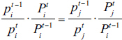
In the Arrow-Debreu economy, the non arbitrage condition, although not explicitly stated, is actually identically fulfilled by present value prices of the different commodities. In fact, present value prices have the property that the return on a loan in terms of good i must be equal to the return realized from the more complex operation of exchange at the beginning of the period of good i with good j, in the subsequent loan denominated in terms of goodj, and in the further retrade at the end of the period of goodj for good i:

(2.8)

where the small-letter p_j^t−1 and p^t_j denote the beginning and end of period present value prices. Remembering that the relative price of any two commodities in terms of discounted values is the same as in terms of undiscounted or current values, indicated by the corresponding capital letters (Burmeister, 1980, p. 13), we have

2.9

Rearranging terms, (2.8) becomes therefore

(2.10)

As the ratio of current to future discounted prices defines the own rate of interest, while the ratio of future to current undiscounted prices defines the rate of inflation in terms of the specific commodity considered, we can rewrite (2.10) as

(2.11)

where own rates ρ_i and inflation rates π_i are defined over the time period t. By approximation, we finally obtain

(2.12)

which shows that: (i) the rate of return on any commodity, considered as an asset, is equal to the sum of the own rate plus the capital value appreciation or depreciation and (ii) the rates of return of any two commodities are equal.

The level at which they are equalised depends on the choice of numeraire. Let n be the numeraire commodity and r its own rate of interest. The properties defining the numeraire are that: (i) its undiscounted prices are equal to one in every period¹⁰ (P_n^t = 1) and (ii) its discounted price at the beginning of the horizon, here t−1, is also equal to one (P_n^t−1 = 1). On account of the first of these properties, the rate of return on the numeraire commodity is equal to its own rate of interest

(2.13)

which in equilibrium is the common rate of return of all commodities. Then, letting j be just any commodity, from (2.12) and (2.14), the non arbitrage condition implicit in the Arrow—Debreu model takes the form

(2.14)

As is clear from the above derivation, in the Arrow—Debreu approach, the own rate of interest is defined with exclusive reference to the discounted prices to a given commodity. When the commodity considered is, however, a capital good, the usual way to define the own rate of interest is not through the ratio of the current to the future discounted purchase price of the durable good, but rather through the ratio of the rental rate of the service supplied by the capital good (which is a flow variable) to the purchase price of the capital good (which is a stock variable). Following this more conventional approach, the percentage rate of return on any capital good j must then satisfy, in equilibrium, the non arbitrage condition expressed in terms of undiscounted prices

(2.15)

where the first term in the right-hand side of (2.15) is the undiscounted rental rate, which is supposed to be paid at the end of the period, as a percentage of the initial purchase price, and the second term is the percentage capital gain or loss on the purchase price of the asset. Using equations (2.9) and the definition (2.13) of the own rate of interest on the numeraire commodity, (2.15) can be expressed in terms of present value prices and rental rates¹¹ as

(2.16)

The relationship between the conventional and the Arrow—Debreu way of defining the own rate of interest can now be readily derived from equation (2.16). Rearranging terms, we obtain

(2.17)

This shows that the ratio of the rental rate to the purchase price is indeed equal to the own rate of interest, when account is taken of the different times to which the variables refer.

Equation (2.16) suggests two further considerations. First, the formulation of the condition of uniformity of the rates of return does not require us to think in terms of a rate of interest. The common interest factor is implicit in the use of present value prices; the equality of the rates of return is thus expressed with the sole reference to the asset prices and the rental rates of each capital good. This may appear at first sight odd, but it really is not. The variables — asset prices and rental rates — relating to each capital good incorporate all the information required for an efficient allocation of resources. This means that, in equilibrium, consumers may safely hold their wealth in just any capital good.¹² Second, and most important, (2.16) exhibits the relation of interdependence that links, in equilibrium, the rental rate to the purchase prices of capital goods. It is this interdependence, which is specific to capital goods, that is not made explicit in the Arrow—Debreu approach, and its role will be investigated in the following sections of the paper.¹³

I have suggested (Tosato, 1997) that the different way to express the own rate of interest in the Arrow—Debreu model as compared with Walras’s theory may simply reflect a difference in the classification of commodities: the accent being on the distinction between commodities available in different time periods, in the former; between capital goods and their services, in the latter. In effect, the conclusion could be somewhat sharper, in the sense that the omission of equation (2.16) implies that the specific nature of capital goods is not properly recognised in the standard formulation of the intertemporal general equilibrium model: prices of capital goods and of their services cannot be independently determined.

3 The model

3.1 Description of the economy

We consider a two-period economy; the generalisation of the model to any finite number of periods is straightforward. With a notation consistent with that used in the preceding sections of the paper, beginning of the period variables are indicated with the superscript t − 1 to distinguish them from the end of period variables, which are denoted by the superscript t. We suppose that there are complete spot and forward markets, which are open at the beginning of the horizon considered, i.e. at time t = 0. Obligations entered into at t = 0 are subsequently carried out at the end of period 1 and in period 2.

The production process taking place in each period is of the point-input—point-output type. Inputs, represented by the services of M capital goods and N primary factors of production, e.g. various types of labour, are applied at the beginning of each period, while outputs, represented by L consumption goods and M newly produced capital goods, are obtained — in a sense that will be clarified — at the end of each period. We make the usual assumption that one unit of any productive resource generates one unit of service and suppose, for simplification, that there is no depreciation on capital goods. No pure intermediate goods are considered; Kehoe (1982) has, however, shown that the model can be generalised to also encompass this case. Firms maximise profits at given market prices in the production set determined by the known technology.

At the beginning of the horizon (t = 0), consumers have strictly positive endowments of M capital goods k_m⁰(m = 1, 2, …, M) and of N primary factors of production (labour) ω_n⁰ (n = 1, 2, …, N) and will have new endowments ω_n¹ of the same primary factors at the beginning of period 2. We assume that consumers do not have a reservation demand for the services of their endowments and maximise an intertemporal utility function.

For the purpose of defining consumers’ behaviour, we assume that consumers rent to the firms the services of their primary factors, for which we obviously do not envisage the possibility of selling the corresponding human capital. This possibility exists, however, for capital goods, so that there are alternative ways — corresponding to alternative institutional arrangements of the working of the economy — in which the individual budget constraint can be constructed.

We could think that consumers lease to the firms only the services of the initial capital goods constituting their endowment, purchase at the end of period 1 the newly produced capital goods and rent again — now at the beginning of period 2 — the services of the old and of the new capital goods and purchase at the end of the same period the capital goods currently produced. But, if we were to adopt this approach, it would be necessary to model consumers’ demand for capital goods also at the end of period 1, and this would substantially require us to operate with separate budget constraints for each of the two periods.

We could, alternatively, suppose that, at t = 0, there exists a market for capital goods in which consumers sell to firms their initial endowments in exchange for financial assets, say bonds, that earn the market rate of return.¹⁴ Consumers then carry out the subsequent wealth adjustments necessary to realise their optimal consumption programme in the two periods, in terms of financial wealth; each consumer can thus either reduce his initial wealth, selling, with delivery at the end of period 1, part of his initial stock of bonds or increase it, buying forward either old bonds from other consumers or, from firms, the new bonds representing the value of newly produced capital goods. Note that in this approach firms maintain, at the beginning of period 2, the ownership of the capital goods purchased at t = 0 and of the investment goods produced in period 1. Only at the end of the two-period horizon do all capital goods — the initial ones plus the newly produced ones — return into the possession of the consumers in exchange for the bonds issued by the firms at t = 0 and at t = 1. This requires that the budget constraint at the individual and at the market levels be appropriately defined.

The approach now considered has two main advantages. First, it easily accommodates the possibility for any consumer to reduce, if he so desires, his initial wealth. Second, there is no need to model consumers’ demand for capital goods at the end of period 1, but only the economy’s demand for capital goods at the end of period 2: and this, as discussed in Section 2.4, is made up of the desired terminal stocks of all capital goods but one, which is residually determined by consumers’ wealth decisions. The absence of a demand for end of period 1 capital goods requires, however, an appropriate formulation of the technology matrix, so that the investment goods produced in period 1 be available, together with those produced in period 2, to be transferred to the consumers only at the end of the horizon.

The definitions adopted here of consumers’ net demand functions and firms’ net supply functions reflect this second approach. We will show that, with the non arbitrage condition, the formulation of consumers’ aggregate budget constraints in terms of sale of the initial stocks is equivalent to supposing that consumers rent the services of the initial endowment of capital goods to the firms for the two-period horizon and receive, in each period, the corresponding rental rates.

3.2 Consumers’ behaviour

We are going to model consumers’ behaviour in terms of properties of market demand functions rather than in terms of properties of individual utility and demand functions. It is nonetheless useful to go through the exercise of deriving the individual budget constraint in present value terms and show the connection between this formulation and that of the constraint that must be met by market demand functions. Using Kehoe’s (1980) terminology, this constraint — which we will, for short, call the market budget constraint — represents a formulation of Walras’s law with reference to the consumer side of the economy.

Let c_h^t be the flow vector of consumption goods (l = 1, 2, …, L) available to consumer h (h = 1, 2, …, H) in period t, and A_h^t be the stock of net wealth of consumer h at the end of period t. Let P^t and Q^t be the current value purchase prices of consumption goods and end of period capital goods; W^t and V^t the current value rental rates, respectively, of capital goods and primary factors. Let also the corresponding lower-case letters a_h^t, p^t, q^t, w^t and v^t stand, respectively, for the present value of net wealth and the present value purchase prices and rental rates. We can write the budget constraints faced by a typical consumer in periods 1 and 2 as

(3.1)
(3.2)

where r¹ and r² are the market rates of return, Q⁰·k_h⁰ is the consumer’s initial wealth, and A_h² is his terminal wealth.¹⁵ The resulting intertemporal budget constraint, as of t = 0, is

(3.3)

This intertemporal budget constraint (3.3) can be transformed from current value purchase prices and rental rates to present value purchase prices and rental rates, obtaining¹⁶

(3.4)

Individual demands,¹⁷ exhibiting nonnegative entries for commodities received by the consumer and nonpositive entries for the value of the capital goods sold and the services of labour rented to the firms, are represented by the vector (c_h¹, c_h², a_h², q⁰·k_h⁰, −ω_h⁰, −ω_h¹). The optimal choice depends on the price vector (p¹, p², q⁰, v¹, v²). Notice that we can consider the difference a_h² − q⁰·k_h⁰ as the individual net demand for wealth to hold at the end of the horizon.

As we move from the individual to the market level, account must, however, be taken of the institutional setting previously described — regarding consumers’ sale of capital goods at the beginning of the horizon to the firms and consumers’ purchase from firms of the stocks available at the end of the horizon — and of the transversality conditions regarding terminal stocks mentioned in Section 2.4. At the individual level, the initial endowment of k⁰ capital goods enters the budget constraint as initial wealth; at the market level, as the economy’s endowment of capital goods, transferred to the firms for the two-period horizon. This means that consumers as a whole have a net offer of capital goods at the beginning of period 1, which is repeated at the beginning of period 2. At the end of the horizon, old and newly produced capital goods are sold by the producers to the consumers, with the implication that terminal wealth of the economy must be equal to the value of the terminal stocks of the various capital goods

(3.5)

with k² ≥ 0.

Turning now to the transversality condition, the remarks made in Section 2.4 become at this stage relevant, namely that M − 1 terminal capital stocks must be exogenously fixed, while the Mth one is residually determined by consumers’ wealth decisions. The vector of desired terminal stocks can thus be specified as

where the vectors ² and ² coincide with the vectors k² and q² after dropping the last element, and ² denotes the prescribed terminal stocks of the first M−1 capital goods. Letting now z = k² − k⁰, the net demand for terminal capital goods can be expressed as

(3.6)

Market demands are then represented by the J = 2L + 3M + 2N vector function

(3.7)

where the f(·) terms are the components expressing the demand for consumption goods and terminal stocks, and the other terms are the supply to firms of the initial capital stocks for two periods and of the services of labour.

Aggregating the individual budget constraints (3.4), we have

(3.8)

which, taking account of (3.5) and of the definition z = k² − k⁰, becomes

(3.9)

To make the aggregate budget constraint consistent with the formulation of the market demand functions, it is necessary to consider the non arbitrage condition (2.16). Repeated application of the latter yields the relation q⁰ − q² = w¹ + w². Substituting in (3.9), we finally have

(3.10)

which is in line with the description (3.7) of the market net demands. This shows that the market budget constraint that consumers’ net demands must satisfy can be formulated in two equivalent ways: the first — equation (3.8) — stresses the circumstance that consumers sell their initial endowment of capital assets to the firms and buy them back only at the end of the horizon; the second — equation (3.10) — points, more traditionally, at the fact that consumption and net terminal stocks decisions are constrained by consumers’ income as determined by renting the services of the endowments of the initial capital stocks and labour.

Let (π, Φ) be the vector of present value prices and rental rates, with components π = (p¹, w¹, v¹, p², q², w², v²) ∈ R₊^J and Φ = (q⁰, q¹) ∈ R₊^2M. In view of (3.10), market demands (3.7) are a function of the subset of prices π and thus a mapping f: R₊^j → R^J.

We make the following assumptions on consumers’ demand functions:

(A.1) Differentiability. Let Z denote a subset of the boundary of the price set R₊^J, including the origin, defined as Z = H ∪ {0}, with H = {π ∈ R₊^J|p¹ = p² = q² = 0}. Then, f(π) is a continuously differentiable function defined on the domain R₊^J/Z.

(A.2) Boundedness from below. f(π) is bounded from below on R₊^J/Z, withf_c¹(·), f_c²(·), f_z²(·), ≥ 0.

(A.3) Desirability of commodities. If πⁱ → π with πⁱ ∈ R₊^J/Z and π ∈ Z/{0}, then ||f(πⁱ)|| → ∞.

(A.4) Homogeneity. f(π) is homogeneous of degree zero.

(A.5) Walras’s law. f(π) satisfies the aggregate budget constraint (3.10), that is 3.11 π·f(π) = 0

Assumptions (A.3), (A.4) and (A.5) are standard, while (A.2) underlies that fact that endowments are finite and that a negative demand for consumption goods is meaningless, as would be a negative demand for net wealth acquisition when a reduction of the initial capital stocks is not physically possible. Assumption (A.1) on the contrary — taken over from Kehoe (1982) — requires explanation. The presence of endowments of capital goods and primary factors of production unelastically supplied by the consumers requires special care in the formulation of the differentiability assumption. Suppose that the only positive prices are the purchase prices of initial capital goods and the rental rates of the primary factors of production; then, if f(π) is in fact continuous, we would have a violation of the aggregate budget constraint (3.10). Note that, on account of (A.3), equilibrium could never occur on the part of the boundary of the price set that has been excluded. Note further that the possibility that some of the endowments will not be fully utilised is not ruled out.

3.3 Production activities

We consider a production technology of the linear activity analysis type without joint production (Koopmans, 1951). As is usual with a constant returns to scale technology, the specification of the production set of individual firms is irrelevant for the study of equilibria; all that matters is the aggregate technology.

The production technology of the economy is described by the (2L + 3M + 2N) × (2 + 2 + 2M + 2N) block matrix A

(3.12)

Positive coefficients refer to outputs, and negative coefficients refer to inputs; empty entries indicate blocks of zero coefficients.

The form attributed to the technology matrix is unusual and needs explanation. The blocks in the first three rows refer to outputs and inputs, respectively, made available and used in period 1; the blocks in the last four rows refer to outputs and inputs made available and used in period 2. The blocks in the first four columns refer to activities carried on in period 1, the remaining four columns to activities performed in period 2. Reading the matrix by columns, it is convenient to start from the latter. Activities in period 2 have no outputs or inputs referring to period 1: this accounts for the blocks of zero coefficients in the upper part. As regards the lower part, the first two columns, i.e. columns five and six of the matrix A, indicate the set of ≥ L activities producing consumption goods and the ≥ M activities producing new capital goods, while the final two columns denote the free disposal activities of the services of capital goods and primary factors. As we have assumed that there are no initial endowments of consumption goods and newly produced capital goods, there is no need to consider disposal activities also for these commodities.

As to the first four columns of the matrix A, column one refers to the production of consumption goods, which is self-contained in period 1, as are the disposal activities of columns three and four. Column two reflects the assumption that capital goods effectively produced in period 1 are actually received by the saving consumers only in period 2. The production activity described by column two of the matrix A uses inputs −A₃₂ and −A₄₂ of services of initial capital goods and primary factors and produces investment goods that are, by assumption, available for sale to the consumers only in period 2 (and this accounts for the first entry A₂₂ in the lower part of column two), and services of these capital goods that can be used for production purposes in period 2 (and this accounts for the second A₂₂).

Let y = (y_c¹, y_z¹, y_k¹, y_ω¹; y_c², y_z², y_k², y_ω²) be a vector of nonnegative activity levels. Aggregate net production, or net supply, is then Ay, and net profits are π·Ay. The output of investment goods is, accordingly, A₂₂y_z¹ + A₂₂y_z², demand for services of capital goods in period 2 is A₂₂y_z¹ − A₃₁y_c² − A₃₂y_z² − Iy_z² where the positive term A₂₂y_z¹ indicates the contribution of the first-period production of investment goods to meet the second-period demand for services, and net profits of the activities that produce investment goods in period 1 are − w¹·A₃₂ − v¹·A₄₂ + q²·A₂₂ + w²·A₂₂.

We make the following standard assumption about the matrix A.

(A.6) Boundedness. No output is possible without input, i.e. {x ∈ R^I | x = Ay ≥ 0, y ≥ 0} = {0}, with I = 2( + + M + N) . Equivalently, there exists a strictly positive price vector π such that π·A < 0, i.e. unit profits are negative.

3.4 Equilibrium

An equilibrium for the economy described by the net demand functions f and by the technology matrix A − in short the economy (f, A) — is a price vector (, ) ∈ R₊^J × R₊^2M/Z that satisfies the following conditions:

(i) there exists ≥ 0 such that f() = A;

(ii) · A ≥ 0;

(iii) purchase price and rental rates of capital assets satisfy the non arbitrage condition ^t−1 = ŵ^t + ^t with t = 1, 2;

(iv) (, )e = 1, where e is a vector of all one.

Condition (i) requires that consumers’ net demand be equal to producers’ net supply. Condition (ii) means that no activity makes positive profits in equilibrium. Condition (iii) is the competitive condition of uniformity of the rates of return on all assets previously defined in equation (2.16). It is convenient to write the non arbitrage conditions in matrix form. Accordingly, let B and C be the block matrices, respectively, of dimensions J × 2M and 2M × 2M:

(3.13)

We can then write (2.16) as

(3.14)

Condition (iv), finally, is the normalisation rule.

The non arbitrage condition has already been extensively commented. Here it may be nonetheless useful, returning to an issue discussed in Section 2.1, to reconsider the role of the non arbitrage condition for capital goods in temporary or permanent excess supply. If a capital good m is in excess supply over the entire horizon, its rental rate w_m^t is always nil, and so are the purchase prices q_m^t. Such a capital good is not an economic good and could be dropped from consideration without altering the equilibrium configuration of the economy. If a capital good m is, on the contrary, only temporarily in excess supply, obviously in the initial stages of the horizon, its rental will at a certain point become positive, say from period τ onward. Equation (2.16) would then imply that the purchase price q_m^τ−1 must also be positive, as will be all the preceding purchase prices q_m^t, down to the very beginning of the horizon. This means that a capital good in temporary excess supply is always an economic good in view of its future scarcity.

4 Existence of equilibrium

To prove the existence of equilibrium, we take advantage of an analytical construction due to Todd (1979) and used by Kehoe (1980) to construct a continuous, single-valued mapping of the price set to itself, whose fixed points are equivalent to equilibria of the economy (f, A).

Let Δ be the unit simplex

(4.1)

Because of the homogeneity assumption (A.4), we can restrict attention to demand functions f(π) defined on Δ/Z.

The first step to take is to extend the definition of these demand functions on the entire price set Δ. This can be done, as Kehoe (1982) shows, using appropriate techniques. We will take this result as given and consider henceforth the net demand functions f(π) to be defined on Δ.

Consider now the subset Δ_A ⊂ Δdefined by

(4.2)

As the intersection of closed and convex sets, Δ_A is a non-empty, closed and convex subset of Δ. To help the intuition, we give in Figure 6.1 an idea of the subset Δ_A. Consider the four-components price vector (p¹, q¹, w¹, q⁰). Using the normalisation rule p¹ + q¹ + w¹ + q⁰ = 1, the four-dimensional simplex can be reduced to the three-dimensional tethraedon ABCO, whose vertices are, respectively, the points p¹ = 1, w¹ = 1, q¹ = 1 and q⁰ = 1. Consider then the non-positive profits constraint p¹a₁₁ − w¹a₂₁ ≤ 1. This reduces the admissible region to the truncated volume

Figure 6.1

A¹B¹C¹OBC. Rewriting the non-arbitrage condition q⁰ = w¹ + q¹ as 1 = p¹ + 2w¹ + 2q¹, it is seen that this in turns restricts the admissible region to the triangle AB²C². The intersection of these two admissible regions is the shaded area B²C²C³B³, i.e. Δ_A.

Let N be any nonempty, closed and convex subset of R^N. Consider the projection map p^N: R^N → N defined by the rule that associates any point x ∈ R^N with p^N(x), which is closest to x in terms of Euclidean distance. In view of the assumed convexity of N, the mapping p^N is continuous.

Using this idea, define now the map g: Δ → Δ by the rule (see Figure 6.2)

(4.3)

As composition of two continuous maps, g(π, Φ) is also a continuous map, in fact a continuous map of the nonempty, compact and convex set into itself, which by Brouwer’s theorem has some fixed points.

Figure 6.2

Proposition 1. (, ) is an equilibrium for the economy (f, A) if and only if is a fixed point of the map g(π, Φ).

We begin by showing the sufficiency part of the proposition, i.e. that, if (, ) is a fixed point, it is also an equilibrium. By definition of projection map, (ψ, ) = g(π, Φ) is the unique solution to the quadratic programming problem

(4.4)

subject to

(4.5)
(4.6)
(4.7)

where the constraints of the optimisation problem reflect the equilibrium conditions (ii)–(iv). Thus a fixed point is an equilibrium if condition (i) is also satisfied.

By the Kuhn—Tucker theorem, there exists nonnegative multipliers y and multipliers λ and μ such that the solution to the programming problem (4.4) must satisfy the following conditions:

(4.8)
(4.9)
(4.10)

Now, let (, ) be a fixed point of the map g(π, Φ), and , , are the associated values of the multipliers. This means ψ = and = , so that (π, Φ) satisfies the following conditions:

(4.11)
(4.12)
(4.13)

Multiplying (4.11) by and (4.12) by and summing, we obtain

(4.14)

Observe now that, as a solution to the problem (4.4), (π, Φ) satisfies the nonarbitrage condition ·B = ·C and, in view of assumption A.5, ·f() = 0. As a consequence of these properties and of condition (4.13) (the Kuhn—Tucker condition), (4.14) becomes

(4.15)

which, on account of (4.7), has a unique solution = 0. Substituting in (4.12), we obtain = 0. We thus see that a fixed point satisfies conditions

(4.16)
(4.17)

which show that the fixed point (, ) is a competitive equilibrium with zero profits.

To prove the necessary part of proposition 1, we show that, if (, ) is an equilibrium, then it is also a fixed point. Let (, ) be a competitive equilibrium. This means that it satisfies the equilibrium conditions (i)–(iv), i.e. f() = A, ·A ≤ 0, ·B = ·C and (, )e = 1. We have to show that it also satisfies the conditions (4.16) and (4.17) for a fixed point. Now, (4.16) is satisfied by definition of equilibrium and (4.17) from (4.16) and Walras’s law. Therefore, f() = A, and (, ) ∈ Δ_A is equivalent to (, ) = g(, ).

As we have just seen, = 0 at any fixed point, with the implication that the constraint represented by the non arbitrage conditions is not binding inasmuch as fixed points must satisfy the constraint. In other words, the non arbitrage conditions (3.14) simply determine the purchase price of capital goods q⁰ and q¹, given p², w¹ and w². This circumstance confirms, in the context of a formal analysis, the validity of the conclusion reached in Section 2.3. The non arbitrage conditions only play the role of determining appropriate, i.e. equilibrium, prices for the initial capital stocks, while the end of period purchase prices are determined by the competitive conditions concerning the newly produced goods. The interesting aspect that the two-period model reveals is that the nonpositive profit constraint is relevant for the determination of the equilibrium configuration only with regard to the final period of the horizon. The competitive conditions concerning the production of new capital goods in the remaining intermediate periods is implicitly taken care of by the condition of uniformity of the rates of return.

The existence of equilibrium of the intertemporal model under consideration can therefore be analysed eliminating altogether the variables Φ, which do not play a role in the determination of demand and supply functions, and concentrating the attention uniquely on the subset of prices π. Adopting a normalisation rule limited to this subset of prices, let

(4.18)

and

(4.19)

where the same notation as in (4.2) is justified by the fact that the two sets are the same up to the normalisation rule.

Define now the projection map (π):Δ_π → Δ_A by the rule

(4.20)

With a procedure analogous to that used before to study the map g(π, Φ), we can now establish the equivalence between fixed points of (π) and equilibria of the economy.

5 Regular economies

A regular economy is one whose equilibria are locally unique and vary con tinuously with the underlying data (f, A). We will approach the study of regular intertemporal economies in an intuitive way.

Let us make the following non-degeneracy assumptions:

(A.7) No column of the matrix A can be expressed as a linear combination of fewer than J other columns.

(A.8) Let A() denote the submatrix of A whose columns are all those activities that earn zero profits at . At any equilibrium, all activities _A making zero profits are operated at strictly positive levels, i.e.f() = A()_A , with _A > 0. Let J′ be the number of these activities.

With these assumptions, the role of which will soon become clear, we can rewrite the equilibrium conditions in the form of equations. Renormalising, for convenience, prices so that π_J = 1 and using Walras’s law to drop the equilibrium condition concerning the market of the Jth commodity, we can write the system of equations of the model as

(5.1)
(5.2)

where the last element of the price vector π has now been set equal to one, and , denote the demand functions and technology matrix obtained by deleting, respectively, the last element and the last row.

We can now think of the problem of the determination of the equilibrium of the economy in terms of counting equations and unknowns. As already indicated, the 2M equations (5.2) — the non arbitrage conditions — constitute a self-contained block whose role is to determine the 2M prices of capital goods in t = 0 and t = 1. As the matrix C is non-singular, the solution is uniquely determined. We must then concentrate our attention on the (J − 1) + J′ equations (5.1). We have, first, to make sure that the number of equations is equal to the number of unknowns. Assumption (A.8) serves this purpose, as it implies that the number of unknowns cannot be less than the number of equations. We must, then, check for the linear independence of the equations. In view of the nonlinearity of demand functions, the question can be examined only in terms of a linear approximation. Consider the linear tangent mapping ξ(π, y): R^J−1 × R^J′ → R^J−1 × R^J′ defined by the (J − 1) + J′ block matrix

(5.3)

We see that this is the Jacobian matrix of the functions defined in (5.1), whose zero is the equilibrium of the economy. This, then, is the condition for the system of equations (5.1) to be locally linearly independent; assumption (A.7) is here directly relevant. If the Jacobian matrix (5.3) is non-singular, the equilibria of the economy are isolated.

Kehoe (1980, 1982) has shown that the following propositions hold for a production economy basically similar to the production and capital formation economy considered in this paper:

(i) under assumptions (A.7) and (A.8), the map (π) is differentiable at its fixed points;

(ii) the sign of the Jacobian matrix associated to the zero of the projection mapping (π) is the same as the sign of the Jacobian matrix associated to the zero of the system of equations defining the intertemporal equilibrium:

(5.4)

(iii) for almost every economy, in an appropriately defined topological structure, det[I − D_π(π)] ≠ 0; this means that, if we choose the parameters defining the economy — i.e. the parameters defining the demand functions and the technology — from a large enough finite-dimensional set, then the probability that the resulting economy is regular is equal to one; in other words, almost every economy has a finite number of isolated equilibria (fixed points);

(iv) the index of the fixed points of a regular economy is a topological constant equal to +1, with the implication that the number of equilibria is odd.

We can therefore conclude that, given an appropriately defined topological structure on the space of intertemporal economies E, almost every inter temporal economy (f, A) ∈ E has a finite number of equilibria, whose qualitative properties are stable under small perturbations of the parameters.

6 Sequential trading and the problem of the determinacy of equilibrium

6.1 Indeterminacy of equilibrium with a linear technology and inelastic factor supplies

The regularity approach to general equilibrium theory shows that competitive equilibria are generically determined, in the sense that, for almost every configuration of parameters, the equilibria are locally unique. This property holds for models of production with linear activities — with limited or even no possibilities of factor substitution — and inelastic factor supplies. Section 5 has shown how the inter -temporal model with capital accumulation considered in this chapter shares this regularity property.

In a series of papers, Mandler (1995,1999a, 1999b) claims that such a regularity argument applies only to intertemporal models, which, in Hicks’s spirit, are rigorously interpreted as descriptions of an economy in which production and exchange decisions take place once-and-for-all at the beginning of time. But, following Radner’s (1972) approach, mentioned in Section 2.2, the intertemporal equilibrium configuration of the economy can be viewed as the result of trading at a sequence of dates, in which current decisions depend on factor endowments, totally or partially inherited from the past decisions, and on a redetermination of the intertemporal equilibrium prices for the remaining periods of the fixed horizon initially envisaged. The reason for the possible resulting sequential indeterminacy lies in the consideration that, while the perturbation argument regarding factor endowments can be legitimately applied to factor supplies from the point of view of the beginning of the horizon, when factor supplies can be considered to be arbitrarily given, this can no longer be done in later periods, as factor endowments are, at least in part, generated by decisions taken by the agents in previous periods. In other words, economies may be driven over time precisely to that combination of factor endowments with which a continuum of equilibria is associated.

Mandler’s argument goes back to one of the two critical remarks made by von Stackelberg (1933) about Cassel’s version of the Walrasian general equilibrium model, which was the object of intense debate at Menger’s Seminars in Vienna in the early 1930s. In order to focus on the origin of the problems of the existence of equilibrium and its determinacy, it is convenient to refer directly to Mandler’s general presentation of the issue (Mandler, 1999a, pp. 26–27). Let a one-period production and exchange economy be described by the following system of equations:

(6.1)
(6.2)
(6.3)

where x(·), y_l and p_l are, respectively, the quantity demanded, the quantity produced and the price of the consumption good l (l = 1, 2, …, L); e_m and w_m the endowment and the rental rate of input m(m = 1, 2, …, M). Equations (6.1) and (6.2) are market clearing conditions, respectively, of consumption goods and factors of production, while equations (6.3) require that all production activities make zero profit.

Stackelberg observed that, if M > L, (6.2) has more equations than unknowns. He consequently remarked that, for typical, i.e. generic, values of factor endowments, there could be no solution of Cassel’s general equilibrium model. The answer to this critical remark is, as is well known, the introduction of slack conditions, which establish that factors in excess supply at the equilibrium configuration have a zero rental rate. Stackelberg further considered, however, the possibility that, still with M > L, a solution could nevertheless exist, with the implication that full employment of all factors could be achieved with the production of a number of commodities less than M. Examining from this perspective the solution of the system of equations (6.1)–(6.3), one can then think of commodity prices as being determined by the market clearing conditions (6.1), where the number of equations is equal to the number of unknowns, and of rental rates as determined by the solution of the remaining zero profit conditions (6.3). But, in the case under consideration, the system (6.3) would have more unknowns (M) than equations (L) and would, therefore, admit of a continuum of solutions, with the con sequence that the equilibrium would no longer be isolated.

Mandler contends that this situation could robustly occur in a model of intertemporal equilibrium with sequential trading. I will consider Mandler’s argument using his neat example, which is highly effective in conveying the gist of the argument, but also in showing its limits.

6.2 Sequential indeterminacy in a two-period intertemporal model

Consider a two-period economy with one consumption good, corn, and two factors of production, corn and labour. The economy starts off in period 1 with a given endowment ₁ of corn, which can be immediately consumed (y₁) or can be saved to be used as seed (₁ − y₁) for the production of corn y₂ in period 2. The technology for the production of corn requires the use of both corn as seed and labour, the endowment of which ₂ in period 2 is supposed to be exogenously given. The production set of the economy is thus defined by the following weak inequalities:

(6.4)
(6.5)

where a₁ and a₂ are the technical coefficients. The frontier of the set (see Figure 6.3) is represented by the piecewise linear function ACD. Point A corresponds to a situation in which all the corn initially available is used for immediate consumption; moving away from A, increasing amounts of corn are used as seed; the kink point C shows the only combination of consumptions y₁ and y₂ consistent

Figure 6.3

with full employment of both corn and labour; thereafter, labour becomes the limitational factor.

To write the zero profit condition in terms of present value prices, we follow the same notational convention adopted in Section 3.2, namely capital letters for undiscounted prices and small letters for discounted prices. In terms of undiscounted prices, we have

(6.6)

where W₁ and W₂ are the rental rates of corn and labour in period 2. As corn used in production is a circulating capital, its rental rate is simply

(6.7)

Thus, passing from undiscounted to present value prices, we have

(6.8)
(6.9)

Assume, for convenience, the existence of a representative consumer. The intertemporal budget constraint in terms of discounted prices is

(6.10)

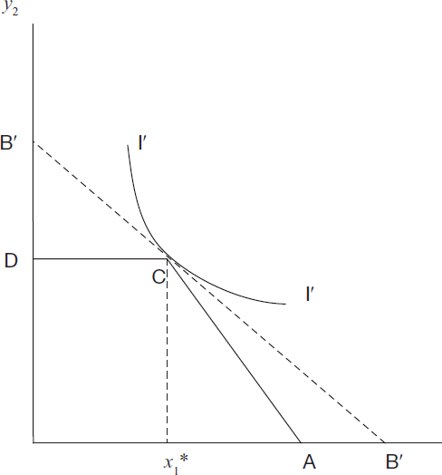
Figure 6.4

where x₁ and x₂ indicate consumption in periods 1 and 2 and ₁ = ₁ is the endowment of the consumption good in period 1.

A graphical representation shows the type of competitive equilibria that can occur. Let p₁ be the numeraire of the price system; according to (6.8), also the discounted price of corn as factor of production in period 2 is then equal to one. Utility maximisation requires the consumer to be on some point of his budget constraint. Thus, for a competitive equilibrium to exist, the budget constraint must have at least one point in common with the frontier of the production possibility set. Depending on the representative consumer’s preferences, this can occur either along the segment AC, implying w₂ = 0 and p₂ = a₁ (see the partially dashed line BB in Figure 6.3), or at point C implying in this case w₂ > 0 and p₂ > a₁, as shown by the dashed line B′B′ in Figure 6.4.¹⁸ In the latter case, the equilibrium price is determined by the slope of the indifference curve I′I′ at C and w₂ is defined by the zero profit condition.

Both types of equilibrium thus determined are regular. To see this at an intuitive level, consider a small perturbation of factor endowments, techno logical coefficients and of the indifference curves. Any such small change of parameters alters the equilibrium position described by Figures 6.3 and 6.4 in the sense that prices, or quantities or both would change; the equilibrium may remain on the flat portion of the production possibility frontier or at the kink point, or move in either direction, depending on the change of parameters considered. This shows that the equilibrium is isolated and that it changes in a differentiably continuous way in response to such parameter changes.

More formally, and in line with the argument of Section 5, let the utility maximising demand functions be x₁(p₁, p₂, w₁, w₂) and x₂(p₁, p₂, w₁, w₂). Letting again p₁ be the numeraire and eliminating by Walras’s Law the market clearing conditions for x₁, the system of equations defining the equilibrium of the model economy considered is, with the same notation as in Sections 3 and 4,

(6.11)
(6.12)
(6.13)
(6.14)
(6.15)

The intertemporal equilibrium model thus consists of five relations — the market clearing conditions, the rental rate of corn as seed and the zero profit conditions in the production of corn in period 2¹⁹ — in the same number of unknowns: (p₂, w₁, w₂ y₁, y₂).

Differentiating the system of equations (6.11)–(6.15) with respect to the unknowns and evaluating the derivatives at the equilibrium position (₂, ŵ₁, ŵ₂), we obtain the Jacobian matrix

(6.16)

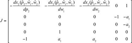
whose determinant is

(6.17)

From the zero profit condition we have dw₂/dp₂ = 1/a₂. Thus the regularity of the equilibrium configuration requires that the ratio of the effects of small variations of p₂ and w₂ on the demand of corn in period 2 be different from this ratio.

If we now pass to examine the hypothesis of sequential trading, we must consider the second-period equilibrium in isolation, taking in particular as given the corn consumption-saving decision of period 1 and thus the availability of corn as a factor of production in period 2. This circumstance determines a major change in the formulation of the equilibrium conditions for period 2: the rental rate of corn w₁ ceases to be linked to the first period price of corn and becomes a variable to be determined together with the production y₂ and the price p₂ of corn, as well as the rental rate of labour w₂. Maintaining the use of small letters, though unnecessary, for the price of corn and the rental rates of factor inputs, setting p₂ = 1 and dropping, on account again of Walras’s Law, the market clearing condition for corn, the second-period continuation of the two-period intertemporal model is described by the factor market clearing conditions

(6.4′)
(6.5)

where ₁ stands for the second-period endowment of corn, and the competitive zero profit condition

(6.9′)

It is now apparent that, if the first-period consumption decision leads the economy to the kink point C in Figure 6.4, the resulting situation is precisely that envisaged by Stackelberg: the production equations (6.4′) and (6.5)) admit of a solution consistent with full employment of both factors, so that a continuum of equilibrium values of the rental rates w₁ and w₂ is generated by the equation (6.9′). As nothing excludes the possibility that the intertemporal equilibrium be at point C in Figure 6.4, the continuation equilibrium of the sequential trading model can be indeterminate.

The Jacobian matrix of the equilibrium system (6.4′), (6.5) and (6.9′) is

(6.18)

whose determinant is clearly zero. This shows that the continuation equilibrium at the kink C is not regular. As a consequence, the equilibrium may change in a discontinuous way. A small perturbation of the endowment of labour or of the technical coefficients of production will make one of the two inputs in excess supply, and its price would drop to zero. The equilibrium position would thus change in a discontinuous way.

Mandler draws two consequences from this circumstance. The first is that even agents that are small with respect to the market would have an interest in manipulating their factor supply so as to force the price of the other factor to zero. Price-taking behaviour would then become implausible. The second consequence, which is strictly linked to the first, is that, if agents are uncertain as to the prices that may rule in period 2, their behaviour in period 1 also may differ from that envisaged by the perfect competition model. The risk of a hold-up situation and the opportunity of an idiosyncratic behaviour on the part of some agents are, therefore, inherent in the sequential trading approach to the intertemporal equilibrium model with a linear technology and endogenously determined factor availability.

An answer to these considerations is that the intertemporal model with sequential trading does not seem to offer a proper description of an economy in which there is a possibility of opportunistic behaviour. Assume that factors inherited from past decisions are fixed capital goods that must be inelastically supplied, thus determining the possibility of an opportunistic behaviour of labour suppliers. The point is that it would be implausible to assume that investors are unaware of such a risk. Opportunistic behaviour would have to be built into the model from the very beginning — for instance through an appropriate formulation of the supply function of labour and of the rental rates of capital goods — and not left to make its appearance only in the second period. Apart from this, and more fundamentally, we know that the market answer to the risk of hold-up is the commitment to long-term contracts, which in the absence of uncertainty can offer a complete description of all possible situations. Hicks’s idea of a pure future economy free of exogenous uncertainty, in which all contracts are entered into at the beginning of time and sub sequently faithfully carried out, may now appear a bit less farfetched than it did at first sight: long-term contracts are really the operational tool by means of which current decisions leaving a legacy for the future are taken.

6.3 Sequential indeterminacy in a three-period intertemporal model

Mandler further states that sequential indeterminacy applies to intertemporal equilibrium models of any number of periods in the very specific sense that ‘each date might represent a multi-period composite, with the two dates forming a partition of a larger underlying set of time periods’ (Mandler, 1999b, p. 12). In other words, should indeterminacy occur in any time period, the equilibrium configuration of all subsequent periods would be indeterminate. This generalisation does not seem to be correct.

Consider a three-period extension of the two-period economy previously examined. The economy starts with a given endowment of corn; the part of it not directly consumed is used as input, together with an exogenously given quantity of labour, for production in period 2. The same linear technology is available for production of corn in period 3.²⁰ The input of labour is again exogenously given, while the input of corn is endogenously determined as the difference between output and consumption in period 2. The entire output of period 3 is consumed.

With an immediate extension of the notation previously used, where e_it and w_it denote, respectively, the quantity and the rental rate of input i (corn and labour) in period t (periods 2 and 3), the system of equations defining the intertemporal equilibrium of the model economy is

(6.19)
(6.20)
(6.21)
(6.22)
(6.23)
(6.24)
(6.25)
(6.26)
(6.27)
(6.28)

Equations (6.19)–(6.20) are the market clearing conditions for the output of corn in periods 2 and 3; by Walras’s Law the market clearing condition of period 1 has been eliminated, and the price of corn in period 1 has been set equal to 1. The market clearing conditions regarding the inputs of corn and labour are formulated as the weak inequalities (6.21)–(6.24) so as to leave the possibility of excess supply of the exogenously given input, labour. With equations (6.25) and (6.27), the discounted value (rental rate) of corn as input is set equal to the discounted price of corn as output in the preceding period. Finally, equations (6.26)

Figure 6.5

and (6.28) establish the competitive condition that no production can make positive profits.

The consumption possibility set is described in Figure 6.5.²¹ Intertemporal equilibrium can occur only on the face ABCD, for otherwise the rental rate of corn would be zero in period 2, implying that the price of corn in period 1 would have to be equal to zero as well. The edge point C represents the only equilibrium with full employment of both factors of production in both periods 2 and 3, with positive prices of all inputs.

If we think of demand functions as being the result of utility maximisation by a representative consumer, indifference surfaces could be (but are not) drawn in Figure 6.5. Nothing prevents the intertemporal equilibrium of the model taking place precisely on the edge point C. The regularity of such equilibrium, intuitively plausible as that at the kink point C of the two-period model considered in Section 6.2, can be established studying the Jacobian of the system.

Let us look now at the hypothesis of sequential trading when the intertemporal equilibrium (_t, ŵ_it, _it, ê₁₃) is precisely in C. Under the assumption of perfect foresight, the first-period consumption decision corresponds to the first-period decision ₁ of the intertemporal equilibrium. The continuation model, now embedding a situation of potential indeterminacy, is expressed by the following system of eight equations in the same number of unknowns:

(6.29)
(6.30)
(6.31)
(6.32)
(6.33)
(6.34)
(6.35)
(6.36)

Compared with the full three-period intertemporal model, in the continuation model involving periods 2 and 3, the market clearing condition regarding the output of corn in period 2 is omitted on account of Walras’s Law; the price of corn in period 2 is accordingly chosen as the new numeraire; the input of corn in the same period 2 is now rigidly defined by the consumption-saving decision previously made, and its rental rate ceases to be linked to the price of corn in period 1. Indeterminacy now occurs in the Stackelberg-Mandler sense: only one variable, namely y₂, appears in equations (6.30)–(6.31), so that the remaining six equations are not sufficient to determine a unique solution for the other seven variables. There is, in particular, indeterminacy of the rental rates of corn and labour in period 2. The argument, however, is not complete unless we consider also what may happen in period 3.

Assume that period 2 sequential trading prices are set equal to the cor responding intertemporal prices ŵ₁₂, and that consumers correctly anticipate period 3 equilibrium prices (₃, ŵ_i3). Then, in period 3, corn and labour would again be available in such quantities as to admit full employment of both. We would be back to the situation of the two-period intertemporal model with sequential trading, with the consequence of no indeterminacy in period 2 and indeterminacy in period 3.

Assume, on the contrary, that the input prices of the period 2 sequential trading approach are set at values different from the corresponding inter temporal equilibrium prices. This would lead the maximising consumer to make a consumption-saving choice in period 2 different from that he had initially planned to make and to anticipate a consumption decision in period 3 equally different from the initially planned one. In particular, the decision as to the quantity of corn to be set aside in period 2 in order to be used as input in period 3 would not be independent of the values assigned to the rental rates w₁₂ and w₁₃. By construction, only if these rental rates coincide with the intertemporal equilibrium values would a situation arise leading to potential indeterminacy. If the potential continuum of equilibria is exploited to generate rental rates w_i2 ≠ ŵ _i2, the availability of inputs in period 3 would no longer be compatible with the full employment of both corn and labour, and the equilibrium of the period 3 continuation would be fully determined, with one of the rental rates having a zero value.

We can therefore conclude that, in the presence of a continuum of equilibrium rental rates in period 2, there is only one price selection — namely that corresponding to the intertemporal equilibrium values — that leads to indeterminacy in period 3. All other selections lead to a modification of the availability of corn in period 3, so that full employment of both corn and labour would not be feasible. In other words, exploiting the potential indeterminacy of rental rates in period 2 makes rental rates uniquely determined in period 3.

Summing up, given an intertemporal equilibrium model with a number of periods t ≥ 2 and considering the associated sequential trading model, rental rates indeterminacy in the sequential realisation is indeed a robust possibility, as Mandler has pointed out. But the horizon cannot be partitioned, as Mandler suggests, in a set of initial periods in which no indeterminacy occurs and in a subsequent set of periods characterised by pervasive indeterminacy. At most, indeterminacy can occur at alternate periods, possibly with a lesser frequency.

7 Paradoxical behaviour

7.1 Capital theoretic critiques of intertemporal equilibrium

The modern controversy on capital theory centres on the question of the implications of reswitching of techniques for the neoclassical theory of value, distribution and growth. Piero Sraffa shows, in his Production of commodities by means of commodities (1960), that the heterogeneity of capital goods and of capital structures, i.e. different proportions between the inputs of labour and of inter mediate goods in the various processes of production, would generally give rise ‘to complicated patterns of price movements with several ups and downs’ (Sraffa, 1960, p. 37). As a consequence, reswitching of techniques may occur, with the implication that the direction of change of the input proportions cannot be related unambiguously to changes in factor prices. This undermines the neoclassical proposition that a fall in the rate of interest is associated with a rise in the capital labour ratio in the production of commodities, on account of the assumed substitutability in production.

Neoclassical economists of the general equilibrium school have no difficulty recognising that the discovery of reverse capital deepening points to an important deficiency of traditional theory and thus requires us to abandon the approach to value and distribution based on the concept of aggregate capital and monotonically decreasing demand functions for both inputs. They argue, however, that the Sraffa-based critique does not apply to general equilibrium models with heterogeneous capital goods and point to the internal consistency of models of Walrasian derivation, in particular to the internal consistency of the intertemporal equilibrium model.

Criticism of the intertemporal equilibrium model comes from several directions. (i) The assumption of complete forward markets is rightly considered unrealistic; but I believe that, at this highly abstract level of the analysis, the problem is one of internal consistency rather than realism. (ii) Schefold (1985) points to a conceptual problem that would be inherent in the possibility of some of the initial endowments of capital goods being in excess supply. This possibility would indicate that entrepreneurial expectations held at some time in the past, before the beginning of the horizon considered by the model, have not been fulfilled. Excess supply of some stocks would thus reveal a situation of disequilibrium, in terms of unrealised expectations, and this ought to influence future behaviour. If future allocation is settled once and for all by means of forward trading, ‘why did this foresight not exist yesterday to prevent the wrong stocks from accumulating?’, Schefold remarks. My reaction is that one could think of several reasons: a change of preferences or of technology, such as the discovery of a new process or a new product. Truly, Schefold’s objection does not appear to be as compelling as he believes it is. (iii) In intertemporal models, own rates of interest are generally different, as relative prices may change in time. This is viewed as a departure from the traditional method of analysis based, first, on the long-term equilibrium or, equivalently, on the long period position and, second, on comparative statics as the tool for the study of change. Furthermore, the change in relative prices is considered to be a source of confusion, inasmuch as it is alleged that it would be difficult to distinguish the permanent from the occasional causes of such price changes. Without entering the debate started by Hahn as to which theory is a special case of the other, it is apparent that structural change can best be dealt with in a model that allows for the systematic possibility that relative prices may change and that clearly accounts for this change, without any possible confusion between permanent and occasional causes. Garegnani (1990) has suggested the logical possibility to extend the classical approach in this direction. I have expressed doubts as to the feasibility of such a step, especially with reference to Garegnani’s statement that, having admitted the possibility of variations in the relative prices of capital goods, one could still distinguish an adjusted from an unadjusted physical composition of the capital stock.

Let me turn to the criticism of the intertemporal equilibrium model directly linked to the reswitching of techniques. Reverse capital deepening (and employment opportunity reversal) may, according to Schefold (1997, 2000) and Garegnani (2000), imply equilibria with implausible features and instability: in a word, a situation of paradoxical behaviour.

7.2 Schefold’s immigration scenario

Schefold constructs a utility function of a representative consumer capable of supporting any feasible consumption path — given arbitrary initial endowments and required final stocks of commodities — as a unique competitive equilibrium. On this basis, he considers alternative perturbations of the equilibrium under the headings of what he calls an ‘immigration’ and a ‘saving scenario’ and investigates if the new equilibrium can be reached under a plausible adjustment mechanism. A typical conclusion is the following: ‘An inter temporal equilibrium with reswitching is thus possible according to the saving scenario, but only if the ordinary neoclassical relation between factor prices and intensities is dropped and if a specific instability is admitted’ (Schefold, 1997, p. 496).

In order to examine Schefold’s argument, I will concentrate on a particularly simple version of his model and, precisely, on the comparison of stationary intertemporal equilibria before and after the shock due to the sudden increase of the labour force — the immigration scenario. Though this comparative statics approach fails to do justice to Schefold’s study of the problems of transition and convergence to the new intertemporal equilibrium, it appears to be adequate to bring out the implausibility of the assumptions that Schefold is compelled to make in order to associate a new intertemporal equilibrium in the presence of reswitching of techniques to the new set of factor endowments.

Schefold considers an economy with only one consumer and a linear technology in which commodities are produced by means of commodities and labour, which is supposed to be inelastically offered. The initial endowments and terminal quantities of all commodities are assumed to be given. In this context, Schefold’s approach consists of: (i) the construction of feasible equilibrium paths of gross and net (consumption) outputs; (ii) the definition of a system of discounted prices of commodities and labour so that activity levels and prices meet the competitive condition of absence of positive profits; (iii) the determination of a suitable utility function that attains a maximum for the given time path of consumption on the consumer’s intertemporal budget set.

Let us now assume, in the immigration scenario, that full employment of labour is possible only with the adoption of a new technique involving reswitching, and let us follow Schefold in considering the new stationary intertemporal equilibrium paths involving constant net outputs before and after reswitching. As a consequence of the change of techniques, not only distribution but also relative prices of commodities will change so as to continue to fulfil the competitive zero profit condition. This, in fact, is the essential implication of reswitching. Contemporaneous relative prices, as well as intertemporal relative prices, associated with the equilibrium obtaining after the shock, will therefore be different from those initially ruling.

In order to prove that these new time paths of quantities and prices constitute an intertemporal equilibrium, is it now necessary — following Schefold’s three-step approach — to show that the unchanged composition and time profile of consumption is willingly demanded by the single consumer of the economy as a utility-maximising bundle on the new budget set.

Schefold suggests that the multiplicatively separable utility functional

(7.1)

where c_i^t and _i^t, respectively, represent current and equilibrium consumption of commodity i at time t, and p_i^t repesents its price, is the appropriate analytical tool.

The utility functional (7.1) has three peculiar properties. First, marginal utility

(7.2)

is on the equilibrium path, with c_i^t = _i^t, identically equal to p_i^t. Second, the contem poraneous marginal rate of substitution in consumption between commodities i and j at time t

(7.3)

is on the equilibrium path identically equal to the contemporaneous relative price ratio p_i^t/p_j^t. Third, the intertemporal marginal rate of substitution

(7.4)

is on the equilibrium path identically equal to the intertemporal relative price ratio p_i^t−1/p_i^t.

However, such a utility functional is clearly implausible. Accepted consumption theory draws a neat distinction between quantities, on which the ranking of alternative consumption bundles is made, and prices that contribute with endowments to determine the budget constraint. The inclusion of both quantities and prices as arguments makes it hard to determine its status: it is neither a direct nor an indirect utility function. The consequences of the joint presence of quantities and prices in the utility function fully emerge from the implication to be derived from the definitions (7.2)–(7.4) of the marginal utilities of consumption and the marginal rates of substitution. The same consumption bundle, with respect to composition and time profile, obtaining before and after the immigration shock, is willingly held by the agent at different relative prices. To put it differently, the shape of the indifference curves along the same intertemporal path of consumption changes according to the price ratio.²²

The lack of plausibility of the assumption made by Schefold as to the form of his utility functional motivates a critical conclusion as to the validity of his results regarding the possibility of paradoxical behaviour of the intertemporal general equilibrium theory, as such results are strictly conditioned by that assumption.

Garegnani’s out-of-equilibrium adjustment²³

Garegnani approaches the question of paradoxical behaviour from a different angle. He constructs what he calls general equilibrium saving and investment functions, by a procedure that amounts to solving implicitly for all the unknowns of the system in terms of the rate of interest, which is the remaining variable to be determined by the saving—investment equality. He then states that, with re switching, the investment function of a circulating capital model has the same characteristics as a demand function for capital in value terms, and that the saving function is backward bending. It follows that some of the intersections of the saving and investment functions correspond to unstable equilibria.²⁴ Perturbation of the equilibrium caused by shifts of the saving function may therefore lead to the para doxical situation of an economy with a zero wage or a negative profit rate.

The out-of-equilibrium adjustment process considered by Garegnani is, however, based on a crucial assumption, hard to justify in itself and the implications of which seem to strongly condition the result of his analysis.

Garegnani considers a two-period, two-commodity general equilibrium model. Arbitrarily given endowments of commodities a and b in period 1 are in part consumed and in part used as productive inputs. New quantities of commodities a and b, to be entirely consumed, are produced in period 2 by a linear technology with those inputs and a given quantity of labour. Market demands, depending on the price system and on the initial endowments, describe the consumption side of the economy.

Whereas Schefold examines the effects of a shock, Garegnani’s aim is to model the out-of-equilibrium behaviour of the economy. With the assumption that period 2 output markets always clear, the study of disequilibrium behaviour concerns the first-period markets of goods a and b and of labour. A standard tâtonnement process would thus involve the discounted prices of these commodities. With the dynamic adjustment functions satisfying a linear equality descending from the budget constraint, it is then sufficient to consider the tâtonnement process with reference to only two of these three variables.

It is apparent that no particular role can be played in this context by the saving—investment market. Saving and investment functions can, of course, easily be defined in terms of present value prices. An investment excess demand function could thus take the place of the excess demand function of either commodity a or b in the tâtonnement process. But the essence of the problem would remain unchanged. In particular, no role could be assigned in the analysis of out-of-equilibrium paths to the interest rate, which does not appear at all in a context of discounted intertemporal prices.

To rescue a role for the interest rate in the study of the adjustment process, Garegnani is compelled to pass from discounted to undiscounted prices. With say commodity a being the numeraire in both periods, the place of its price in the adjustment process is taken by the interest rate. Following, therefore, a line of reasoning similar to the preceding one, a tâtonnement process could now be envisaged with reference to the saving—investment market and the market of one of the commodities. The out-of-equilibrium paths of the interest rate and of the price of commodity b would have to be accordingly determined. In particular, the dependence of saving and investment on second-period consumption demands makes counterintuitive behaviour of the saving and investment functions in response to the interest rate possible, thus opening the door to a multiplicity of equilibria, instability and paradoxical behaviour of the wage rate and of the interest rate.

The point is, however, that in order to establish the existence of paradoxical behaviour Garegnani makes a peculiar assumption — his equation (1.7f) (Garegnani, this volume, p. 20). In the study of out-of-equilibrium paths he imposes the condition that the ratio of the demands of commodities a and b, including both consumption and productive uses, should always be equal to the ratio of the corresponding endowments. This implies that the adjustment process in one of the two markets considered is specified directly in quantity terms, rather than as a function of relative prices, as usually done in a standard tâtonnement analysis. This mixing of a price and quantity adjustment in the same model is far from clear; the reasons for assuming price rigidity in one market (commodity a) and price flexibility in the other (the saving—investment market) ought to be better argued. It is hard to accept, on this basis, Garegnani’s conclusion that paradoxical behaviour is the necessary outcome of the presence of reswitching of techniques in production.

Summing up, it may well be that reswitching of techniques and capital reversal may lead to unstable equilibria and counterintuitive adjustment processes when judged from standard neoclassical theory. Neither Schefold nor Garegnani seem, however, to have been able to produce a convincing critique of traditional theory in the papers here taken into consideration.²⁵

A final comment with regard to the nature of the Sraffa-based critique of intertemporal general equilibrium theory: Garegnani has claimed that the instability due to the Sraffian critique of the general validity of the principle of factor substitution in production is qualitatively different from, and more relevant than, the instability originating from perverse income effects in consumption. Although the latter have always been known to exist and have been considered as true exceptions of limited interest to an otherwise general norm, the former is a new and unsuspected phenomenon, not of zero measure in probability terms, which cannot be considered as a mere exception. The failure of the principle of substitution in production would thus compel neoclassical theory to be abandoned altogether.

Actually, a positively sloped demand for a production input is hardly distinguishable, from an analytical point of view, from a positively sloped demand for a consumption good. They are both the result of the presence of complementarity, in one instance, in consumption, in the other, in production (Hatta, 1990). The outcome is the same: multiplicity of equilibria and instability may equally well arise in both cases. If we want to use the term paradoxical behaviour to denote these situations, then paradoxical behaviour is certainly possible in intertemporal models: it is the consequence of the structure of the economy, not of the theory.

8 Conclusion

We have tried to show in Section 2 that the intertemporal general equilibrium model is the natural setting for the study of the problems raised by the presence of saving and investment, problems that Walras had tried to tackle within his static approach. With the assumption, crucial for the theory, of arbitrarily given quantities of heterogeneous capital goods, the non arbitrage condition of equality of the rates of return — defined as the ratio of the rental price of the initially available durable goods to the cost of production of the new means of production — may fail to hold. The exclusion of possible capital gains or losses, implicit in Walras’s hypothesis that the prices of old and new capital goods are the same, precludes in general the possibility of fulfilling the condition that the percentage rates of return on all capital goods be equal.

The consideration of what Lindahl aptly called the ‘time factor’, which Walras had neglected in the construction of his model of capital formation, resolves the apparent contradiction in the context of a fully specified inter temporal model.

One such simple model, making explicit the aspects of capital accumulation and the presence of the competitive condition of equal rates of return on all durable goods, is presented in Section 3 and analysed in Sections 4 and 5. Under appropriate, but not very restrictive, assumptions, the existence of equilibrium is proved, as well as the generic property of regularity (i.e. of determinacy) of equilibria.

Nothing is said about the number of equilibria and their stability. In models of pure exchange economies, uniqueness depends on the property of commodities being gross substitute in consumption; in this case the equilibrium is also stable.²⁶ The questions of uniqueness and stability are considerably more complex in pro duction economies. The possibility of complementarity among factors of production plays a role similar to that of complementarity in consumption, paving the way for multiplicity and instability.

Multiplicity, instability and, more generally, paradoxical features are said to be exhibited by intertemporal general equilibrium models when the possibility of re switching of techniques and capital reversal is reckoned. Schefold’s and Garegnani’s models, which aim at proving such a possibility, are critically examined. A careful analysis shows that their results depend on an implausible assumption (Schefold) or on a debatable procedure in the study of out-of-equilibrium paths (Garegnani).

This does not mean that multiplicity and instability of equilibria may not occur in production as well as in pure exchange economies. It simply means that the Sraffian critique of the general validity of the principle of factor substitution in production, based on the possibility of capital reversal and reswitching, does not seem to be able to offer grounds for the claim that a new, more relevant and basic reason has been discovered for the failure of the neoclassical general equilibrium theory to produce unique and stable equilibria.

A different line of criticism has been proposed by Mandler, who argues that the regularity proposition applies only to models of a pure futures economy. When, more realistically, the intertemporal configuration of equilibrium is viewed as the result of trading at a sequence of dates, indeterminacy can robustly occur. While agreeing that such a possibility may result as a consequence of the endogeneity of factor availabilities in periods following the first, we observe — contrary to Mandler’s statement — that the time horizon envisaged by the model cannot be partitioned into a set of initial periods in which no indeterminacy occurs and a subsequent set of periods in which indeterminacy is pervasive. Indeterminacy of equilibria can occur, at most, at alternate periods, possibly with a lesser frequency.

Mandler draws a further and more fundamental critique of the competitive equilibrium model from the possibility of indeterminacy inherent in the sequential trading approach. He calls attention to the fact that indeterminacy may induce even small agents to have an interest in manipulating their factor supply so as to force the price of other factors to zero. Opportunistic behaviour of this type would lead to questioning the very assumption of competitive equilibrium.

Granted that the possibility of opportunistic behaviour would have to be built into the model from the very beginning, and not allowed to creep in only in a subsequent moment, there is a more relevant consideration to be taken into account. The market answer to the risk of hold-up is the commitment to long-term contracts, by means of which current decisions leaving a legacy for the future are taken. From this point of view, the pure futures economy described by the intertemporal equilibrium model appears to be somewhat less unrealistic and farfetched than it might have appeared at first sight.

Notes

* I am grateful for useful comments to Saverio Frattini, Sergio Nisticò, Fabio Petri, Enrico Saltari and Filippo Vergara Cifarelli. The usual disclaimer applies.

1 Cf. Garegnani (1990, pp. 23–44). In his contribution to the volume of The new Palgrave dedicated to Capital theory, Garegnani has systematically resumed and broadened his critique of the neoclassical theory of capital, both in the aggregate version and in the general equilibrium approach. For the sake of convenience, I shall refer here, when relevant, exclusively to this work.

2 Similar considerations can be found in Allais (1977, in particular pp. 145–57) in the context of a paper highly critical of the approach taken by Arrow and Debreu in their model.

3 All references are to the 1954 English translation made by W. Jaffé on the basis of the definitive 1926 edition of L. Walras, Eléments d’économie politique pure ou la théorie de la richesse sociale, Lausanne, Cobaz.

4 Cf. Garegnani (1990, pp. 4–22).

5 That precisely this circumstance is the discriminating element between the neoclassical and the classical or Ricardian approach has been vigorously stressed by Hahn (1982).

6 This conclusion clearly does not change when, as argued by Garegnani (1990, pp. 47–8) with the definition of the notion of ‘effective rates of return’, one should include in the determination of the rate of return the variation in the supply price of capital goods.

7 The same type of approach can be found in Koopmans (1957) and is implicit, when moving to a context of uncertainty, in the use of the ‘Arrow securities’ which offer ‘insurance’ against the risk of negative states of nature (Arrow, 1965).

8 Generalisations of the competitive equilibrium model in this direction can be found, for instance, in Bewley (1972).

9 Mas-Colell, Whinston and Green (1995, part 4) offer an up-to-date presentation of such techniques.

10 See Radner’s reinterpretation of the Arrow—Debreu economy as a sequence of spot markets plus forward markets in the numeraire commodity.

11 Currie and Steedman (1990, p. 145) present the same equilibrium condition considering the case of land.

12 Currie and Steedman (1990, p. 147) attribute the separation of the decision to hold capital good i from the decision to hold capital good j to the circumstance that all payments must be made at the beginning of the horizon. It is of course true that all contracts must be stipulated and regulated at the very beginning, but the separation of the decisions concerning which capital goods to hold is a consequence of the fact that all transactions are supposed to take place at the equilibrium prices, which fulfil the condition that the rates of return are equal. If transactions were to take place at out of equilibrium prices, this separation would fail to hold.

13 For a similar remark, see Currie and Steedman (1990, p. 145).

14 A similar approach has been adopted by Diewert, who refers — as we saw in Section 2.3 — to the fiction of a financial intermediary sector that purchases the capital goods from households and rents the services to the firms. Diewert’s idea of a financial intermediary sector seems to be less suited to cope with a multiperiod horizon.

15 The notation indicates the inner product of the generic vectors x and y

16 Let l be any commodity and n the numeraire; then

where the first equality follows from the property that the undiscounted price of the numeraire is equal to one; the second follows from equation (2.9); the third follows from equation (2.13); and the last one follows from the property that the discounted price of the numeraire at time zero is equal to one.

17 The term demand is generically used to identify consumers’ behaviour.

18 Note that the equilibrium cannot occur on the flat part CB of the frontier, as this would imply that the marginal utility of corn becomes nil for a finite level of consumption, contrary to the assumption of smooth preferences that underlies the regularity approach to the study of the equilibrium positions.

19 The competitive condition (6.15) in the production of corn is directly stated as an equality condition, as, in equilibrium, the output of corn must necessarily be positive.

20 This is merely a convenient simplification; the technical coefficients could equally well change from period to period.

21 The consumption possibility set no longer coincides with the production possibility set as in the two-period exercise previously considered, on account of the fact that a positive consumption in period 3 requires that part of production in period 2 be with -drawn from consumption.

22 It seems hard to associate this peculiarity of Schefold’s indifference curves to some results on endogenous time preferences (Epstein and Hynes, 1983). In this latter context, the utility functional is always specified exclusively in terms of consumption profiles, and the changing shape of indifference curves is the result of endogenously changing, rather than constant, time preference.

23 My understanding of Garegnani’s approach to the study of out-of-equilibrium paths has greatly benefited from a seminar by my colleague S. Parrinello and the final version of his paper (Parrinello, 2005).

24 It is doubtful that one may consider these intersections as alternatively stable and unstable, as if dealing with only a two-commodity economy.

25 A critique of Schefold’s and Garegnani’s approaches along similar lines can be found in Mandler (2002).

26 Instances of instability of the unique equilibrium configuration of a pure exchange economy are constructed by Scarf (1959) under the assumption of strong complementarity in consumption.

References

Allais, M. (1977), ‘Theories of general economic equilirium and maximum efficiency’, in G.S. Schwodiauer (ed.) Equilibrium and disequilibrium in economic theory, Dordrecht: Reidel.

Arrow, K.J. (1965), Aspects of the theory of risk-bearing, Helsinki.

Arrow, K.J. and G. Debreu (1954), ‘Existence of an equilibrium for a competitive economy’,Econometrica, 22, pp. 265–90.

Bewley, T. (1972), ‘Existence of equilibria in economies with infinitely many commodities’, Journal of Economic Theory, 27, pp. 514–40.

Burmeister, E. (1980), Capital theory and dynamics, Cambridge: Cambridge University Press.

Currie, M. and I. Steedman (1990), Wrestling with time. Problems in economic theory, Manchester: Manchester University Press.

Debreu, G. (1959), Theory of value: an axiomatic analysis of economic equilibrium, New Haven: Yale University Press.

Diewert, W.E. (1977), ‘Walras’ theory of capital formation and the existence of a temporary equilibrium’, in G.S. Schwodiauer (ed.) Equilibrium and disequilibrium in economic theory, Dordrecht: Reidel.

Epstein, L.G. and J.A. Hynes (1983), ‘The rate of time preference and dynamic economic analysis’, Journal of Political Economy, 91, pp. 611–35.

Garegnani, P. (1990), ‘Quantity of capital’, in J. Eatwell, M. Milgate and P. Newmann (eds) The new Palgrave — capital theory, London: Macmillan.

—— (2000), ‘Savings, investment and capital in a system of general intertemporal equilibrium’, in H. Kurz (ed.)Critical essays on Piero Sraffa’s legacy in economics, Cambridge: Cambridge University Press.

Hahn F. (1982), ‘The neo-Ricardians’, Cambridge Journal of Economics, 6, pp. 353–74.

Hatta, T. (1990), ‘Capital perversity’, in J. Eatwell, M. Milgate and P. Newmann (eds) The new Palgrave — capital theory, London: Macmillan.

Hicks, J.R. (1939), Value and capital, Oxford: Oxford University Press.

Kehoe, T.J. (1980), ‘An index theorem for general equilibrium models with production’, Econometrica, 48, pp. 1211–32.

—— (1982), ‘Regular production economies’, Journal of Mathematical Economics, 10, pp. 147–76.

Koopmans, T.C. (1951), ‘An analysis of production as an efficient combination of activities’, in T.C. Koopmans (ed.) Activity analysis of production and allocation, New York: John Wiley & Sons.

—— (1957), Three essays on the state of economic science, New York: McGraw-Hill.

Lindahl, E. (1939), Studies in the theory of money and capital, London: George Allen & Unwin.

Mandler, M. (1995), ‘Sequential indeterminacy in production economies’, JJournal of Economic Theory, 66, pp. 406–36.

—— (1999a),Dilemmas in economic theory, New York: Oxford University Press.

—— (1999b),‘Sraffian indeterminacy in general equilibrium’, Review of Economic Studies, 66, pp. 693–711.

—— (2002), ‘Classical and neoclassical indeterminacy in one-shot versus ongoing equilibria’, Metroeconomica, 53, pp. 203–22.

Mas-Colell, A., M.D. Whinston and J.R. Green (1995), Microeconomic theory, New York: Oxford University Press.

Parinello, S. (2005), ‘Intertemporal competitive equilibrium, capital and the stability of tãtonnement pricing revisited’, Metroeconomica, 56(4), pp. 514–31.

Radner, R. (1972), ‘Existence of equilibrium of plans, prices, and price expectations in a sequence of markets’, Econometrica, 40, pp. 289–303.

Scarf, H.E. (1960), ‘Some examples of global instability of the competitive equilibrium’, International Economic Review, 1, pp. 157–72.

Schefold, B. (1985), ‘Cambridge price theory: special model or general theory of value?’, American Economic Review, 75, pp. 140–45.

—— (1997), ‘Classical theory and intertemporal equilibrium’, in B. Schefold, Normal prices, technical change and accumulation, London: Macmillan, pp. 425–501.

—— (2000), ‘Paradoxes of capital and counterintuitive changes of distribution in anintertemporal equilibrium model’, in H. Kurz (ed.) Critical essays on Piero Sraffa’s legacy in economics, Cambridge: Cambridge University Press.

Sraffa, P. (1960), Production of commodities by means of commodities, Cambridge: Cambridge University Press.

Todd, M.J. (1979), ‘A note on computing equilibria in economies with activity analysis models of production’, Journal of Mathematical Economics, 6, pp. 135–44.

Tosato, D. (1997), ‘Equality of rates of return in models of general economic equilibrium with capital accumulation’, in G. Caravale (ed.) Equilibrium and economic theory, London: Routledge.

von Stackelberg, H. (1933), ‘Zwei Kritische Bemerkungen zur Preistheories Gustav Cassel’, Zeitschrift fur Nationalökonomie, 4, pp. 456–72.

Walras, L. (1874–7), Eléments d’économie politique pure, Lausanne: Cobaz [definitive edition 1926].

——————

COMMENT ON TOSATO

Fabio Petri

1. Owing to space constraints, I prefer to concentrate almost exclusively on the first part of Professor Tosato’s paper, where he discusses Garegnani’s criticism of Walras. Some misunderstandings appear to emerge in that part that can be the occasion for clarifications, which should help the progress of discussion. Only at the very end I advance one comment on the formal part of the paper (on the relevance of the theory of ‘regular economies’), and three brief comments on the criticisms of Schefold and Garegnani in Section 7.

Garegnani’s critique of Walras’s model appears not to have been fully under stood by Professor Tosato. This critique is summarized in Section 2.1 as follows: the absence of a uniform rate of return, admitted by Walras, implies in general a tendency of investment to become concentrated on only some of the capital goods, with a relevant change over time of the composition of capital, ‘with subsequent effects on equilibrium prices and quantities’; the model therefore (reformulated with inequalities, so as to have a solution) identifies only a short-period equilibrium, contrary to tradition and to Walras’s own intentions, which were to determine a long-period position, and is therefore affected by an internal inconsistency between the specification of the capital endowment and the condition of uniform rates of return (‘determined with respect to the reproduction costs’, i.e. on supply price), an internal inconsistency that reflects ‘a contradiction … between the alleged scope of the theory, namely to define a long-period position, and a consistent formulation of it, which is confined to yielding only a short-period equilibrium’.

There are two deficiencies in Professor Tosato’s summary — and, I must suppose, in his understanding — of Garegnani’s critique, that although connected must be disentangled, and allow a better understanding of the arguments in the paper. The first and main deficiency consists of the absence of a discussion of why, according to Garegnani, the fact that Walras’s equilibrium system (modified with inequalities according to Walras’s own indications) cannot identify a long-period position constitutes a reason for substantive criticism of the modified model, in other words, why, according to Garegnani, one cannot be content with short-period general equilibria. The second deficiency, largely a consequence of the first one, consists in locating the main effect of the given vector of capital endowments, and, hence, of the absence of a uniform rate of return, in the impossibility to assume that the relative prices of capital goods do not change over time, which is, on the contrary, what Walras assumes.

There can be no doubt that indeed the solution of Walras’s original model (when it exists) or of his reformulation with inequalities generally implies that the economy will start the following period with a relevantly different composition of capital and, therefore, relevantly different equilibrium prices; and it is a further deficiency of Walras’s model that he neglects these effects on subsequent prices when his own argument implies that these effects can easily be very relevant; but Garegnani’s accusation of contradiction (cf. also Garegnani, 1960, pp. 116–17), although also recognizing this further deficiency of Walras’s model, is centrally based on a different point: that it is contradictory to assume that the tendency toward equality between supply and demand for produced goods and the tendency toward an equal rental for all units of each factor have had sufficient time to operate, and yet that, during this time, the arbitrarily given quantities initially in existence of the several capital goods will not have changed: during the time required to adapt to demand the quantities produced of consumption goods, utilization and production of new capital goods will be going on and altering the endowments of the several capital goods. (The fairy-tale tãtonnement based on ‘bons’ while economic activity is suspended was introduced by Walras in the 4th edition of his Eléments precisely because he finally realized this contradiction betwen his data and his previous description of the tãtonnement as involving actual productions — but the ‘bons’ are only a fairy tale, adjustments take time and involve actual productions, and no theory can be acceptable that does not take this fact into adequate account.) As a result, before the repetition of interactions of buyers and sellers can have the time to correct or compensate the differences between supply and demand on the several markets, the data relative to the capital endowments may have changed considerably, and not in the way predicted by the equilibrium (had the latter been reached instantaneously); thus, the theory gives no reason to expect that the initial equilibrium, or the subsequent sequence of equilibria, will describe with sufficient approximation the trend resulting from the trial-and-error disequilibrium behaviour of agents. This is what I call the ‘impermanence problem’, a central component of Garegnani’s objections, not only to Walras, but more generally to the given vector of initial capital endowments of modern general equilibrium theory in all its versions.

Surprising as it may be in view of the stress put on it by Garegnani (1990), Professor Tosato never mentions this issue. Then, what is left of Garegnani’s criticism of Walras’s reformulated equilibrium is only that it is not a long-period equilibrium, but this is no longer a criticism, because no reason backs the claim that value theory should only aim at determining long-period equilibria. Thus one can go on to ask whether, as a short-period equilibrium, Walras’s model is consistent, and the sole remaining weakness is the illegitimate absence of a consideration of price changes over time. This explains why Professor Tosato can argue that Walras’s inconsistency is surmounted by subsequent neo-Walrasian theory, in particular by intertemporal equilibria. Temporary equilibria with subjective expectations, or intertemporal equilibria with complete futures markets or perfect foresight, can indeed be seen as ways to admit a relevant non-constancy of relative equilibrium prices over time. But both share with Walras the fault considered central by Garegnani, the given vector of capital endowments and therefore the impermanence problem; so Professor Tosato could not have considered them solutions to Walras’s inconsistency if he had fully understood Garegnani’s criticism.

However, the impermanence problem is increasingly admitted to be extremely serious (cf. Petri, 2004, chs. 1 and 2), and it is a pity that we do not have Professor Tosato’s views on this issue. I would argue that only a composition of capital that has become such as to yield a uniform rate of return on supply price can be considered sufficiently persistent (i.e. subject to changes that are sufficiently slow) as not to deprive the corresponding prices and quantities of the persistence necessary for the role of ‘centre of gravitation’, i.e. for the role of good indicator of the average or trend of market prices and quantities. The determination of equilibria that cannot have this role does not constitute an acceptable positive theory of value, distribution or outputs. I would further argue that this position would have met the approval of all the founders of marginalist theory, including Walras (see below), and that therefore his changes in the 4th edition need a more careful consideration than simply a suggestion that he was ‘quite aware of the difficulties that may arise in meeting the condition of uniformity of the rates of return’ and ‘ready to abandon it’¹ owing to ‘analytical rigour as [his] foremost preoccupation and aim’. A different and more convincing explanation can indeed be offered, and I will sketch it below. But even if Professor Tosato’s interpretation were accepted, the question would remain, whether continuing on the road of modern ‘Walrasian’ equilibria is the right choice. The impermanence problem cannot be left out of a discussion of this question.

2. There is, however, also another strand to Professor Tosato’s persuasion that inter temporal equilibria fully surmount Garegnani’s criticism of Walras. In Section 2.2, he reports that he has argued in 1997 that the inconsistency of Walras’s theory lies, not in the arbitrary given vector of capital endowments, but rather in the neglect of the changes of the relative prices of capital goods over time, and that once these changes are admitted — as in intertemporal equilibria — then ‘the variation in relative prices … makes it possible to verify the condition of uniformity of the rates of return, no matter what the composition of the initial endowment of capital goods may be’. (The implication would appear to be that, in this respect, the difference between intertemporal equilibria and long-period positions does not lie in the presence or absence of a uniform rate of return but in the admission or not of changes of relative prices over time.)

It might appear that such a view rests simply on an insufficient distinction between the uniformity of rates of return achieved by intertemporal equilibria and the uniformity of rates of return on supply price that Walras hoped to determine and that is considered fundamental by Garegnani. However, Professor Tosato is clearly aware of the difference between the two. I think I have found an error in his views, but it is a different error. In order to point it out, it is useful first to remember the above distinction.

The uniformity of rates of return in the first periods of Arrow—Debreu intertemporal equilibria is on demand price, not on supply price. For example, if the demand for steel has just dropped, the durable capital goods only used for steel production will be underutilized, and their value (demand price) will fall below their production cost (supply price), which is why production of new capital goods of the same type will be zero. The rate of return on investing in their purchase will be equal to the rate of return on any other form of investment, but because computed on the demand price, not on the cost of production, of those capital goods. The traditional uniformity of rates of return was on the contrary on supply price, and Walras is no different in this respect. It is the uniformity of supply price that Walras is referring to, when he admits that ‘it is probable that there would be no equality of the rates of net income’.²

In the present chapter, Professor Tosato does not discuss this difference directly, but I have cited above a phrase of his where he recognizes that the uniform rate of return discussed by Garegnani is on supply price, and earlier in the paper he discusses the need to ascertain the value of the initial endowments of capital goods in Walras’s model in a way that makes it clear that this value is the demand price of these capital goods. However, in the earlier paper (Tosato, 1997), he appears to have considered the uniformity of rates of return on demand price all that one should ask for, as it means absence of arbitrage opportunities and therefore absence of incentives to change;³ why then now does he not feel the need to clarify that one should not ask for a uniform rate of return on supply price? The answer, it would seem, goes as follows.

He assumes an economy where time is divided into periods, all production processes take one period and are started at the beginning of each period, and prices are defined only for each beginning-of-period (or, equivalently, end-of-the-previous-period) date. Nothing is known on what happened before the date t = 0, when the intertemporal equilibrium is established, therefore (as explained more clearly in Tosato, 1997) the cost of production (supply price) of the capital goods present in the initial endowments cannot be defined; supply prices can only be defined from t = 1 onwards. Therefore the issue, whether the rate of return on supply price is uniform or not, only acquires meaning from t = 1 onwards.⁴ For this economy, Professor Tosato appears to state the following: once changes of relative prices over time are admitted, an intertemporal equilibrium is capable of establishing the uniformity of rates of return on supply price from t = 1 onwards; this shows up in the fact that, from t = 1 onwards, the purchase prices, i.e. demand prices, of all capital goods (which are determined as the present value of subsequent net rentals) coincide with their costs of production: ‘the supply price of the newly produced capital goods … is necessarily the end of period price of the complex of all capital goods, both inherited from the past and newly produced’ (p. 112, section 2.2).

If my interpretation is correct, then Professor Tosato is in error. If the vector of initial capital endowments is arbitrary, it will not be generally possible to reach the equality between demand price and cost of production (supply price) for all capital goods at t = 1, nor for a number of subsequent dates. For example, if a machine’s initial endowment is so abundant that its marginal product is zero in the first period, it may well remain zero, or anyway too low, for a number of periods: it may take considerable time for the scrapping of the oldest machines of the same type to raise the scarcity of that machine. Even circulating capital goods, if not perishable and present at the beginning in too abundant quantities relative to demand, may be only partly utilized in the first period, and their remaining inventories, transferred to successive periods, may be sufficient to satisfy demand for a number of periods, preventing production of new capital goods of the same type until their stocks have sufficiently decreased. Professor Tosato would be right only if all capital goods were produced already in the first period, but this is precisely what Walras admits will not generally happen, if the initial endowments are arbitrary.

Thus, Professor Tosato is mistaken in suggesting that, in intertemporal equilibrium models, the divergence between demand price and supply price is nonexistent as soon as supply price can be defined. The divergence can exist for a considerable number of periods. So, what is fundamental for the possibility of reaching a uniform effective rate of return on supply price (UERRSP) is not the variability of relative prices over time, but the endogenous determination of the composition of capital.

However, once the composition of capital is left free to adapt to demand so as to achieve a UERRSP, then the changes that relative prices may be still undergoing will be generally so slow that the economic theorist will have the right to neglect them, because they will be essentially due to the slow changes in income distribution due to extension of cultivation to inferior lands or, in the marginalist approach, due to changes in the capital—labour ratio because of accumulation and population growth. There is a vast difference in potential speed between these slow changes and the much quicker changes in the composition of capital due to the absence of UERRSP. This is the reason why classical as well as traditional marginalist authors, including Walras, neglected the changes over time of normal relative prices: they (very reasonably) thought that these changes, once the composition of capital had adapted to the composition of demand so as to permit UERRSP,⁵ would be very slow and, hence, generally negligible relative to the speed of convergence of prices toward costs of production; therefore, the assignment of the same price to a good as input and as output was a fully acceptable approximation.

Thus we find that, on the one hand, the changes of relative prices over time admitted by intertemporal equilibria do not allow one to reach a UERRSP; on the other hand, if a UERRSP is assumed, then the composition of capital must be left to be determined endogenously, but then changes of relative prices over time can be legitimately neglected.

3. Thus, when Professor Tosato writes that the attribution of the same price to a good as input and as output is ‘the discriminating element between the neoclassical and the classical or Ricardian approach’ (p. 152, fn. 5), he is not totally wrong (if one intends by ‘neoclassical approach’ modern general equilibrium theory), but he depicts as fundamental what is in fact only a consequence of a consequence of the really fundamental difference.

The real fundamental difference between those two approaches is the view of the determinants of distribution, in particular of real wages. The socio-political forces that determine real wages in the classical approach are persistent enough to allow the assumption that the real wage does not change during the processes of adjustment of the composition of capital that bring about a UERRSP. The consequence is the legitimacy of the attempt to determine long-period positions. Thus, the theory concentrates on long-period prices, and the consequence of this consequence is a legitimate neglect of the changes that these relative prices may be undergoing, because these changes are slow. The aim of the founders of the marginalist/neoclassical approach was, analogously, the determination of sufficiently persistent positions (long-period equilibria), and as long as the supply-and-demand forces postulated by that approach were believed to be able to determine them, the treatment of prices was the same as in the classical authors.⁶ But the determination of wages on the basis of demand and supply forces deriving from given endowments, together with the need endogenously to determine the com -position of capital, obliged these authors to take as given an endowment of capital as a single factor of variable ‘form’, an amount of value (except for Walras who, as will be argued below, was simply less clear than the others on the need endogenously to determine the composition of capital in order to have the right to assume a UERRSP). The consequence was that, when it became clear that the conception of capital as a single factor of variable ‘form’ was indefensible, and that the sole alternative specification of the capital endowment was the one adopted by Walras, the abandonment of the attempt to determine long-period positions characterized by a URRSP became an unfortunate necessity for neo classical theorists. The consequence of this consequence was that, as the theory in its new versions only attempted to determine very-short-period equilibria, it became necessary to admit the possibility of relevant changes of relative prices over time.

Thus, the presence or not of the UERRSP condition is more fundamental than the absence or presence of changes of relative prices over time; it is only another face of the treatment of the composition of capital as endogenously determined, or given; the latter treatment reflects nowadays the modern forms that the neoclassical approach had to take owing to its failure to reach its original aim, the determination of long-period equilibria.

4. The above characterization of the neoclassical shift from long-period to very-short-period versions as an unfortunate necessity is supported by a careful consideration of Walras’s evolution. There is abundant evidence (much of it unearthed by Garegnani, 1962) that Walras initially aimed at determining a long-period general equilibrium and, for a long time (nearly thirty years), he believed he had succeded in this task. Only shortly before the 4th edition of his treatise (1900), i.e. near the end of his intellectually productive life, did Walras become aware of some of the contradictions in his analysis; then he introduced several changes (not in the equations, though) to try and save his theory as best he could: these changes (among them the new description of the tãtonnement as based on bons without any disequilibrium production or exchange, a different description of the process tending to bring about a uniformity of rates of return on supply price; and the unobtrusive admission⁷ that that uniformity would not be generally achievable) resulted in a text full of inconsistencies; in particular, no change was introduced in the role attributed to the equilibrium,⁸ which remained the traditional one of centre of gravitation of disequilibrium prices and quantities, in spite of the admission that it would not be characterized by a UERRSP.⁹

For a detailed presentation of the supporting evidence, I refer the reader to Garegnani (1962) and Petri (2004, Chapter 5). Here I only remember:

• the several passages, surviving up to the last edition, where the equilibrium is characterized in the traditional way as the persistent centre of gravitation of day-by-day prices and quantities;
• the persisting neglect of changes of relative prices over time;
• the fact that, until the 3rd edition (1896) of the Eléments, Walras did not assume that the entire production function of a firm was known in advance, but rather assumed that the marginal products of factors had to be discovered by actual experimentation of variations of factor employments (Petri, 2004, p. 145), something requiring considerable time, and incompatible with the later tãtonnement based on bons;
• the survival up to the last edition of a passage where Walras admits that the tendency of prices toward costs of production is slow (therefore the composition of capital cannot remain unaltered while this tendency operates):

  there never is a day when the effective demand for products and services equals their effective supply and when the selling price of products equals the cost of the productive services used in making them. The diversion of productive services from enterprises that are losing money to profitable enterprises takes place in various ways, the most important being through credit operations, but at best these ways are slow.

  (1954, p. 380; 1988, p. 580)

• the many aspects of the analysis that only make sense in a long-period, rather than in a very-short-period, equilibrium; perhaps the clearest one is the already mentioned absence of any consideration of future price changes in the determination of rates of return; but one may also list: the absence of debts of firms; the absence of a fixed factors/variable factors distinction; the absence of a distinction between modern and obsolete capital goods; also, if well understood, the treatment of the money endowments of agents;¹⁰
• the survival up to the last edition of the following striking passage, noticed by Garegnani (1962), where the uniform rate of return on supply price is clearly described as brought about by changes in the relative endowments of the several capital goods:

  Capital goods proper are artificial capital goods; they are products and their prices are subject to the law of cost of production. If their selling price is greater than their cost of production, the quantity produced will increase and their selling price will fall; if their selling price is lower than their cost of production the quantity produced will diminish and their selling price will rise. In equilibrium their selling price and their cost of production are equal.

  (Walras, 1954, p. 271; 1988, p. 353)

Thus, the most plausible interpretation is that Walras, alone among the founders of the marginalist approach, did not realize that the process bringing about a uniform rate of return on supply price implied that one had to treat the composition of capital as determined endogenously, and was more generally unclear on the implications of a given vector of endowments of capital goods; only between the 3rd (1896) and the 4th edition (1900) of the Eléments he started realizing the contradiction between such a treatment of the capital endowment and his description of how the economy would tend toward equilibrium; he then tried to paper over the cracks of the theory as best he could, without having either the courage openly to acknowledge the faults he had discovered in it or the force to think through their implications.

This is why, also basing myself on Walker’s (1996) observations on Walras’s health problems and declining scientific productivity, in Petri (2004), I conclude:

The changes introduced in the fourth edition are therefore the product of a period when Walras’ capacity to work was limited; they were nonetheless published very quickly; afterwards, Walras was probably incapable of further reflection on them. Thus those changes should not be considered the solid result of years of ponderate reflection. True, Walras was often unrigorous in his reasonings even before; but some of those changes look more like acts, I dare say, of desperation, motivated by the need to salvage a theory in deep trouble. It would be otherwise difficult to understand how Walras could accept, for example, the new tãtonnement based on ‘bons’, which contradicted his aspiration to describe the actual grouping of real economies.

(Petri, 2004, pp. 148–9)

5. As pointed out in Petri (2004, pp. 136–7), this reconstruction of the evolution of Walras’s analysis is important, because it shows that Walras was no exception to the general belief, among the founders of the marginalist approach, that the determination of a long-period equilibrium was the necessary aim of their theory. Garegnani’s thesis, that the long-period method was initially fully accepted by marginalist economists, and was only questioned (and then largely misunderstood and forgotten) when, much later, it became clear that marginalist theory was unable to conform to that method, is fully confirmed. One can then better appreciate the importance, for the success of the approach, of the fact that for several decades it was believed that the approach was perfectly capable of determining long-period equilibria: Walras and Wicksell initially believed so, and when later they recognized problems in their theories, their admissions long went almost unnoticed.

We economists of the twenty-first century, better conscious of the radicality of the shift undergone by the theory of value with the adoption of a Walrasian treatment of the capital endowment and a more consistent adoption of very-short-period notions of equilibrium, can now ask whether the shift has been able to restore consistency to the neoclassical approach to value and distribution. The question here is: what are we to mean by ‘consistency’? It must mean, I would argue, a capacity satisfactorily to explain what determines prices and distribution in real market economies (not in fairy tale economies), which requires models that are both formally and interpretatively adequate.

6. On this issue, as far as intertemporal equilibria are concerned, Professor Tosato is clear, they ‘cannot offer the basis for an understanding of the behaviour of real economies in time’ because of the unreality of the assumption of complete futures markets or perfect foresight (again, the impermanence problem is not mentioned): consistency has not been restored. On the contrary, the fruitfulness of the teporary equilibrium method is not discussed. But when one remembers that, owing to the impermanence problem, the indefiniteness of results due to exogenous unknowable expectations, and the insufficient factor substitutability, even Hicks ended up rejecting that method (Petri, 1991); when one adds the arbitrariness of the assumption that savings determine investment once the notion of a decreasing demand curve for capital, the value factor, is abandoned (Petri, 2004, Chapter 7); and when one also remembers the serious problems with existence of temporary equilibria noticed by the general equilibrium specialists; then the conclusion is clear: consistency has not been restored by the theory of temporary equilibria either. The Walrasian treatment of the capital endowment is as indefensible as the given value capital of Wicksell and Clark. The marginalist/neoclassical approach is inconsistent in all its versions.

I come to my other comments. I asked myself, why did Professor Tosato consider it important to prove that the model he presents in Sections 3 to 5 is that of a ‘regular economy’? He does not explain why, but a plausible conjecture is that he is conscious that multiple equilibria are a serious problem for general equilibrium theory, and he finds some comfort in the claim, advanced by the theory of regular economies, that general equilibrium theory does not yield totally indeterminate results, because equilibria are generically locally isolated. This prompts me to point out that the comforting implications (for the neoclassical theorist) of the theory of regular economies appear to be greatly overestimated.

First, the Sonnenschein—Mantel—Debreu results show that the finite number of equilibria can be very high, and the different isolated equilibria can be very close to one another, so that the degree of indeterminateness can be nearly the same as with a continuum of equilibria.

But this is not all. Professor Tosato states what appears to be the generally accepted view when he writes that, ‘The regularity approach to general equilibrium theory shows that competitive equilibria are generically determined, in the sense that for almost every configuration of parameters the equilibria are locally unique’. Notice how the result is presented: there is no mention of the fact that the result is only demonstrated for ‘differentiable’ economies. Hahn (1993) too presents the result in this way. The assumption, that the consumers’ excess demand function is differentiable (cf. assumption A.1 in Section 3.2 of Professor Tosato’s paper), apparently is considered of minor importance: the result is presented as of general validity. On the contrary, the assumption is extremely restrictive. It comes extremely close to requiring that either a consumer never demands a good, whatever the relative prices, or, if she demands a good in positive amount at some prices, then she demands it in positive amounts whatever the relative prices. This is because if, as the price of a good increases, a consumer reaches a corner solution (her initially positive demand for that good becomes zero), then her demand function for the good will nearly always have a kink at that price, and so it will not be differentiable there.¹¹

The differentiability assumption excludes, for example, the case of Figure 7.1, an Edgeworth box where the endowment point Ω is the unique equilibrium allocation but there is a continuum of equilibrium relative prices: all slopes of the budget line included in between ΩH and ΩK represent equilibrium relative prices.

In this case, the existence of a continuum of equilibrium relative prices is robust with respect to a small modification of preferences, or to a small change in endowments as long as this consists, for each consumer, of a small change in the sole endowment of the good in positive endowment (a restriction that can be reasonable in some situations, e.g. an exchange economy where consumers living in different areas have access to different endowments).

Now, in the real world it is very difficult to think of a consumption good demanded in positive amount for which demand would not go to zero if the

Figure 7.1 The indifference curves of consumer A are drawn as continuous thin curves, those of consumer B as broken thin curves. Ω, the endowment point, is the lower right-hand corner. All budget lines between the thick broken straight lines ΩH and ΩK represent equilibrium relative prices

price rose sufficiently. The implication is that economies with differentiable excess demands (and therefore regular economies too) must be considered highly excep tional; the theory of regular economies is inapplicable to plausible economies.

That the set of economies with a continuum of equilibria is of ‘measure zero’ in the space of possible neoclassical economies (rather than only in the space of ‘differentiable’ neoclassical economies) is therefore a claim, not only of doubtful relevance, because it does not exclude the nearly as damaging possibility of very many equilibria very close to one another, but also still in need of demonstration.

7.  I end with telegraphic comments on some statements in Section 7 of Professor Tosato’s paper.¹²

(a)Schefold pointed out in 1985 that intertemporal equilibria inconsistently assume both complete futures markets or perfect foresight, and arbitrary (and therefore possibly vastly unadjusted) initial capital stocks that reveal unrealized expectations: thus complete futures markets or perfect foresight exist now but did not exist in the past? Professor Tosato replies that ‘one could think of several reasons’ explaining the lack of foresight, for example a change of preferences, or technical progress; but it seems to escape him that if such an unpredictable change of preferences or of technical knowledge occurred in the past then it must be admitted to be a possibility also for the future, and the agents’ choices should take this fact into account, but the equilibrium equations don’t; so Schefold’s accusation of inconsistent asymmetry is confirmed.

(b)Contrary to Professor Tosato’s interpretation, in Schefold’s utility function the scalars indicated with the same symbols as prices are not variables endogenously determined by the solution of the equilibrium equations. Those scalars are given constants. Then, Schefold assumes that by a fluke these constants are just equal to the prices of the intertemporal path he has previously determined, and this is why he uses the price symbols. Under this assumption, he shows that that path is indeed an equilibrium path. The purpose is only to show that there are assumptions on the preference side that can make that path an intertemporal equilibrium path.

(c)In Garegnani, the assumption that the out-of-equilibrium composition of demand for the initial-period commodities is the same as the out-of-equilib -rium composition of supply does not appear to me as arbitrary and unjustified as Professor Tosato suggests. When the rate of return on supply price is uniform on all capital goods, investors are indifferent as to the composition of investment. But an excess demand for a capital good proportionately greater than for other capital goods, inducing in all likelihood an increase in its price and thus a decrease in its rate of return on supply price relative to the rate of return on other capital goods, will tend to redistribute investment toward the other capital goods; this suggests that, if there is excess demand for capital goods, the composition of this excess demand most compatible with a uniform rate of return on supply price is the one assumed by Garegnani.

Notes

1 In this way it is also suggested that it is not true that Walras intended to determine a long-period equilibrium.

2 Walras, 1954, p. 308: §267 of the 4th and 5th edition; cf. also p. 294: §258 of 4th and 5th ed.; for the French original cf. Walras, 1988, pp. 430–1, and p. 401; Jaffé’s translation is sometimes objectionable.

3 Such a view would appear to be, again, the result of an insufficient attention to the impermanence problem: the latter points out that the absence of arbitrage opportunities can only be plausibly assumed for situations where economic agents have had the time to correct, or compensate, previous errors (there is no instantaneous tãtonnement with ‘bons’ in real economies!) and therefore for situations where the composition of capital has had time to adapt.

4 This conclusion depends on the particular assumptions made on production. Supply prices would be determinable also at t = 0, if in all industries production were a continous flow with no lag between flows of input services and emergence of the corresponding output flows.

5 See below in the text for a quotation from Walras showing that he too associated the uniform rate of return condition with an endogenously determined composition of capital.

6 The neglect of the changes of relative prices over time was, in both the classical and the traditional marginalist authors, only a (legitimate) simplification, not a logical necessity of the theory.

7 The two passages where Walras admits that the uniform rate of return on supply price will not generally obtain are indeed ‘unobtrusive’, as shown by the fact that they were not generally noticed until many decades later. In the Preface to the 4th edition, Walras mentioned the change in the description of the tãtonnement (without explaining its motivations: 1954, p. 37), but not the other changes, in particular, not the new admission that a uniform rate of return on supply price could not be generally achieved.

8 Reference is sometimes made to §322 of Walras’s Eléments (1954, p. 380), where Walras describes a shifting equilibrium, as evidence that Walras had in mind a temporary equilibrium. This interpretation forgets that this passage is there from the earlier editions, where it is impossible to deny that Walras was determining a long-period equilibrium; and indeed the remainder of the passage (the example of the lake) again presents the equilibrium as the persistent average around which market magnitudes oscillate; the passage must therefore be interpreted as describing the traditional method of long-period positions, which are never completely reached and are slowly changing all the time.

9 It may even be doubted that the situation of equality between supplies and demands on all markets but without a uniform rate of return on supply price, envisaged by Walras in the passages of the 4th edition where he admits that a uniform rate of return cannot generally be achieved in his model, is considered by him an equilibrium. He writes:

In an economy like the one we have imagined, which establishes its economic equilibrium ab ovo, it is probable that there would be no equality of rates of net income … On the other hand, in an economy in normal operation which has only to maintain itself in equilibrium, we may suppose the last l equations to be satisfied.

(Walras, 1954, p. 308)

The distinction between establishing and maintaining an equilibrium makes little sense, unless the first sentence is interpreted as meaning that the economy without uniform rate of return on supply price is on its way to establishing equilibrium but has not yet reached it, and will establish equilibrium only when the uniform rate of return will be achieved — and only from that moment on, will it only have to maintain itself in equilibrium. Had Walras considered the situation without uniform rate of return on supply price an equilibrium, then he should have described any sequence of such situations as maintaining the economy in equilibrium, because the economy would be in equilibrium in each period.

10 Walras assumes that the money endowment is, at the beginning of each period, entirely in the hands of consumers, and that each consumer ends the period with the same amount of money he started with, a typical assumption in the study of stationary economies. He states, however, that the initial money endowments are ‘random’ (Walras, 1954, p. 318), i.e. of any magnitude; it is then absurd to exclude the possibility that individuals may want to start the following period with a different amount of money balances. Thus here too one finds a contradictory co-existence of long-period and very-short-period elements.

11 For example, let us assume that in a two-good economy a consumer has quasi-linear utility u = (x₁ + 1/4)^1/2 + x₂, and an endowment consisting of 1 unit of good 1. The strictly convex indifference curves are all parallel vertical displacements of any one of them, and they touch the vertical axis with slope equal to −1; so the consumer has positive demand for good 1 only if p₁/p₂ 1. Let us normalize prices by setting p₂ = 1; then for p₁ < 1 the demand for good 1 is given by the solution of

At p₁ = 1, it is x₁ = 0, the right-hand derivative of x₁(p₁) in p₁ = 1 is zero, the left-hand derivative is 1/2, so x₁(p₁) is not differentiable in p₁ = 1.

12 The fact that I abstain from commenting on other parts of the paper does not mean that I have no disagreements with what is said in them. For example, I strongly disagree with the statements (on complementarity and ‘paradoxical behaviour’) in the last paragraph of Section 7, but it would take a full paper adequately to discuss the opinions somewhat cryptically advanced in those few lines.

References

Garegnani, P., 1960, Il capitale nelle teorie della distribuzione, Milan: Giuffrè.

Garegnani, P., 1962, ‘On Walras’s theory of capital’, unpublished ms., distributed at the 1986 CISEP International Summer School, Trieste. Published with title ‘On Walras’s theory of capital (provisional draft 1962)’ in Journal of the History of Economic Thought, 30(3), August 2008, 367–84.

Garegnani, P., 1990, ‘Quantity of capital’, in J. Eatwell, M. Milgate and P. Newmann (eds) The new Palgrave — capital theory, London, Macmillan.

Hahn, F.H., 1993, ‘Sequence economies and incomplete markets’, in Art J. de Zeeuw, Advanced lectures in quantitative economics II, London and New York: Academic Press, pp. 51–79.

Petri, F., 1991, ‘Hicks’s recantation of the temporary equilibrium method’, Review of Political Economy, 3(3), 268–88.

Petri, F., 2004, General equilibrium, capital and macroeconomics, Aldershot: Edward Elgar.

Tosato, D., 1997, ‘Equality of rates of return in models of general economic equilibrium with capital accumulation’, in G. Caravale (ed.) Equilibrium and economic theory, London: Routledge.

Walker, Donald A., 1996, Walras’s market models, Cambridge: Cambridge University Press.

Walras, Léon, 1954, Elements of political economy, Jaffé translation, Homewood, IL: Richard D. Irwin; Augustus M. Kelley reprint, 1977.

Walras, Léon, 1988, Eléments d’économie politique pure: ou théorie de la richesse sociale, Pierre Dockès et al. (eds), Paris: Economica.

——————

REPLY TO PETRI

Domenico Tosato

In my reply to Professor Petri’s comments, I will work my way in reverse order with respect to the one he has followed. I will start, therefore, by examining first the detailed observations that he makes in Sections 6 and 7 of his Comment and turn thereafter to the main argument he develops in Sections 1 through 5, dealing with the interpretation of Walras and with the intertemporal general equilibrium approach to the theory of value and distribution. This choice is not casual: it reflects a personal priority for analytical issues over methodological disputes.

1.. My answer to Professor Petri’s telegraphic comments to some of the statements contained in Section 7 of my paper will be considerably lengthier, also on account of the fact that I have been able in the meantime to examine Schefold’s and Garegnani’s lectures at the 1999 Siena Summer School on General Equilibrium, and the subsequent General Discussion (Petri and Hahn, 2003) and a version of Schefold ‘s (2003b) paper containing a clarifying reformulation of Garegnani’s approach to the problems of stability of intertemporal equilibrium models. I will dedicate particular attention to this latter issue.

1.1 Professor Petri shares Schefold’s accusation of inconsistent asymmetry of general equilibrium theory, which would be implicit in the assumption of arbitrarily given initial endowments of capital goods. If perfect foresight or complete markets are assumed in the model, arbitrary initial endowments of capital goods inherited from the past would reveal unrealised expectations. This would imply that the assumption of perfect foresight, which is supposed to hold for the future, cannot have been valid in the past. Hence, the inconsistent asymmetry of the assumptions.

Professor Petri objects to the reasons supplied in my paper in order to justify that asymmetry — the occurence of unpredictable changes of preferences or technology. He maintains that, if agents have gone through the experience of what they might have considered unpredictable changes in the past, they can no longer continue to hold the same beliefs. Decisions pertaining to the future would accordingly have to take into account, presumably in stochastic terms, the possibility that those events may occur again. However, the equations of the model fail to recognise such a possibility. Thus, Professor Petri concludes, the removal of the inconsistent asymmetry of assumptions about the existence of complete future markets or of perfect foresight would necessarily entail the abandonment of the assumption of arbitrarily given initial endowments of the several capital goods (Petri, this volume, p. 165).

Let me agree on the fact that changes that have been experienced in the past can and should be considered predictable, perhaps in stochastic terms, and thus accommodated in the model. This is precisely what is done in the Arrow—Debreu model with the device of contingent commodities. Each period’s endowments will therefore be stochastically adjusted. But let me observe that the existence of markets for contingent commodities makes it possible for agents to realise an optimum allocation of risk ex ante, i.e. before the shock (state of nature) is revealed. If the shock has economy wide consequences — if it is a macroeconomic shock in Laffont’s terminology (1989, pp. 70–5) — the ex post implications would show up in a disruption of the composition of the capital stock. Suppose that a shock to preferences has occurred in the sense that agents wish to reduce savings and demand a greater quantity of some commodities and a lesser quantity of others. The available capital goods would ex post result in some in short supply and others in excess supply. An external observer (the general equilibrium economist setting up ab ovo his model) would describe the situation as of arbitrarily given endow ments of the several capital goods.

In conclusion, if, for the sake of the argument of eliminating Schefold’s accusation of inconsistent asymmetry, we want to turn the unpredictable changes that occurred in the past into stochastically predictable changes that may occur in the future, I see no compelling reason to abandon on this account the assumption of arbitrarily given initial quantities of capital goods.

The fact that some of the shocks that have occurred in the past may be considered predictable into the future does not mean, however, that all shocks to preferences and technology should be of a predictable nature. It is hard to imagine that past experience may be able to cover all possible contingencies that may arise in the future. When shocks of this kind were to occur, capital goods endowments would result that were appropriate with reference to the old preferences and technologies, but indeed not to the new ones.

1.2 Professor Petri attributes to me a wrong interpretation of Schefold’s utility function — equation (6.1) of my paper. He states that, ‘the scalars indicated [in that function] with the same symbols as prices are not variables endogenously determined by the solution of the equilibrium equations … [but] given constants’ (Petri, this volume, p. 165). Professor Petri admits that only by a ‘fluke’ would these constants be equal to the prices and quantities of the intertemporal path defined on the basis of the feasibility and the competitive conditions of the model. But this would be irrelevant. In line with Schefold’s own statements, he concludes that the purpose has been ‘only to show that there are assumptions on the preference side that can make that path an intertemporal equilibrium path’ (Petri, ibid; see also Schefold, 2000, p. 372).

The answer to Professor Petri’s remark is here twofold. First of all, Schefold clearly states that had he written the utility function in the standard form

(6.1a)

and then shown that the intertemporal path of consumption quantities _i^t and prices p_i^t would be supported as a competitive equilibrium path only if the parameters of the utility function had the values α_i^t = 1 + _i^t and (β_i^t = p_i^t; ‘the reader would have easily realised’ that the form (6.1a) had been constructed so as to yield the desired result (Schefold, 1997, pp. 469-70). In a more recent contribution, Schefold (2003a, p. 444) further writes that his construction goes through ‘if the equilibrium prices and quantities are treated as parameters’ in (6.1).¹ The point is that these are parameters that change in a predictable and not in an arbitrary way. When, for instance, the immigration scenario is considered, the new equilibrium prices and quantities associated with this scenario become the new ‘parameters’ of the utility function. It seems to me that, in the light of these and of the more general observations developed in my paper as well as of Schefold’s own statements, it is not warranted to consider the parameters of the utility function (6.1) as ‘given constants’.

Independently of the interpretation of the symbols in (6.1) as endogenously determined variables, parameters or given constants, Schefold’s utility function — and this is my second remark — has another and much more important role with respect to the one that Professor Petri seems to attribute to it: i.e. simply ‘to show that there are assumptions on the preference side that can make that path an intertemporal equilibrium path’ (Petri, this volume, p. 165). It has the role to show that, when reswitching and capital reversal are admitted, the intertemporal equilibrium model produces paradoxical comparative statics (dynamics) results as in Schefold’s immigration scenario, in which, with an increase in the quantity of labour, by assumption always fully employed, there is associated in equilibrium an increase rather than a decrease in the real wage, as one would, on the contrary, expect on the basis of the neoclassical demand-and-supply approach to the theory of distribution.

Let me first dispel the view that, from the standpoint of general equilibrium theory, this ought to be considered a paradox. The association, in a comparison of equilibrium configurations, of a higher real wage with a higher labour supply is in no sense a paradox because, when demand and supply both shift, the direction of price change can be arbitrary.²

Let me further remark that Schefold is not only quite clear about the role of his utility function, but apparently also dubious about its validity. At the conclusion of the presentation of his model at the Siena Summer School he writes: ‘if the equilibrium exists, it presupposes unplausible preferences and, if these are accepted, it is unstable’ (2003a, p. 448; emphasis added). But why then base the whole model on such ad hoc and admittedly unplausible preferences? With a standard and plausible utility function, Schefold’s paradoxical results, as Mandler (2002) has convincingly argued, would disappear.³

1.3 Professor Petri criticises my remark that Garegnani’s ‘proportionality’ assumption — that the out-of-equilibrium composition of demand for the initial-period commodities is the same as their supply composition — is arbitrary and unjustified. His critique is based on the idea that investors are indifferent as to the composition of investment when the rates of return on supply prices are uniform.

My answer needs here to be rather lengthy as it involves the presentation of some critical remarks on the overall approach Garegnani has taken to the study of stability of the intertemporal equilibrium model in terms of a saving—investment disequilibrium. To this end, I will start by considering Garegnani’s intertemporal equilibrium model — his system (E). I will show that, in a standard tãtonnement analysis of stability with recontracting, no role can be attributed to a disequilibrium between saving and investment. Stability analysis can and should be carried out at the proper microeconomic level; the macroeconomic level of analysis, implied by the approach in terms of a saving—investment disequilibrium, is at best unnecessary and possibly leads to wrong conclusions.

Taking advantage of Schefold’s reformulation, I will then consider Garegnani’s system (F), which describes his approach to stability analysis without recontracting. I will first show that a role for a divergence between saving and investment can be envisaged only by making use of Garegnani’s proportionality assumption, which essentially reduces a multidimensional microeconomic disequilibrium in the endowments markets to a one-dimensional macroeconomic saving—investment divergence. Garegnani’s rationing scheme thus appears to be strictly functional to the goal of reducing the issue of stability to a problem of measurement of aggregate capital and cannot be justified on the basis of Professor Petri’s argument that savers are indifferent among a variety of capital goods offering the same rate of return.⁴ I will then offer some comments on Garegnani’s approach to the problems of stability in terms of what he calls ‘general equilibrium’ saving and investment schedules.

1.3.1 The Hahn—Garegnani intertemporal model describes a two-period economy. At t = 0, the economy starts off with a given initial supply of labour L and given endowments of two commodities, each being both a consumption and a circulating capital good.⁵ For compact notation I will indicate them as A_i0 with i = 1, 2. The economy’s demand for these commodities, the sum of consumption and investment demand, is indicated as A_i0^D. Production is of the point-input—point-output type: inputs used at t = 0 produce outputs A_i1 at t = 1. The technology is assumed to be linear with coefficients a_ij , with i,j = 1, 2, and l_j indicating, respectively, the quantity of commodity A_i0 required to produce one unit of commodity A_j1 and the quantity of labour per unit of output. There are complete markets; three spot markets for the initial endowments of labour and commodities and two forward markets for the outputs of period t = 1. Commodity prices P_j1 and the wage W, which is supposed to be paid at t = 1, are accordingly defined in present value terms as discounted prices at t = 0, while prices of current endowments are indicated as P_i0.⁶ Competition is supposed to rule in the production of both commodities. consumers’ demands for commodities are indicated with the symbols D_i0(·) and D_i1(·), where the dot in the parenthesis stands for all prices including the wage rate; they are supposed to have standard Walrasian properties.⁷ Investment I₀, determined by the needs of t = 1 outputs, and saving S₀, depending on incomes at t = 0, take place only at the beginning of the horizon, as no further economic activity is envisaged thereafter. Commodity 2 at t = 1 is assumed to be the numeraire of the system. The own rate of return r₂ is thus defined in terms of this commodity.

The model is made up of the following 13 equations presented in an order as close as possible to Garegnani’s.

(1)-(2)
(3)
(4)-(5)
(6)-(7)
(8)
(9)
(11)
(12)
(13)

The equations of the model are self-explanatory: (1) and (2) define the competitive condition of zero profits in production; (3) defines the numeraire; (4) and (5) determine the demands for the initial stock of commodities; (6), (7) and (8), with the added slack conditions, impose weak conditions of equilibrium in the markets of the initial endowments and of labour; (9) and (10) impose strict equilibrium conditions in the markets for the commodities produced at time t = 1; investment and saving are defined in value terms by equations (11) and (12); (13) determines the own interest rate on the numeraire commodity through the ratio of discounted prices.

To study the equilibrium of the model (1)–(13), it is sufficient to consider the submodel made of the first ten equations, as the remaining three merely define investment, saving and the own rate of interest, given the price and quantity solution determined by the first subset of equations.⁸ But we will soon return to consider the possible role of these equations. This system (1)–(10) — which I will call the ‘basic intertemporal model’ — coincides with Garegnani’s system (E), were it not for the added presence of the variables A_i0^D, which are not influential for the study of the properties of the model. This basic ten-equation model describes demand and supply conditions in five markets: the three input markets of the initial endowments of commodities and of labour and the two output markets of period t = 1. It contains nine variables: the five prices (of the three inputs and the two outputs), the two demands A_i0 of the initial endowments of the two commodities and the two outputs A_j1. As one of the equations is linearly dependent on the others, one can conclude that, with the standard assumptions on the demand functions, a set of equilibrium prices and quantities does exist. Obviously, the equilibrium solution of the model need not, and in general will not, be unique.

1.3.2    Turning the attention now to the out-of-equilibrium adjustment process, we must consider the implications of Walras Law. The excess demands in the input and output markets of the intertemporal model (1)–(10) satisfy the constraint that their value sum is equal to zero

(14)

Walras Law implies that, if a market is out of equilibrium, there must be a compensating disequilibrium in at least one other market. As (14) represents a fundamental constraint on the study of the out-of-equilibrium adjustment process, I will refer to Walras Law as the disequilibrium structure or representation of the model.

In the model under consideration we may distinguish between intertemporal and infratemporal disequilibria: the former involve compensating excess demands at both t = 0 and t = 1, the latter, only excess demands at t = 0 or t = 1, but not both. In the microeconomic approach of the specific two-period model here considered, an intertemporal disequilibrium involves the excess demand (supply) of one of the current inputs compensated by an excess supply (demand) of one of t = 1 consumption goods. In macroeconomic terms, an intertemporal disequilibrium is a saving—investment disequilibrium in the sense that an excess, for instance, of saving over investment in t = 0 would have to be matched by an excess demand of at least one commodity in t = 1. To substantiate this statement, which is not immediately clear from (14), it is sufficient to notice that, considering now the model including the definitions of saving and investment, from equations (4), (5), (11) and (12) we obtain

(15)

This shows that a divergence between saving and investment is, by definition, the price-weighted algebraic sum of disequilibria between demand and supply of the various endowments. Substituting (15) in (14), we have

(16)

which is Walras Law reformulation in terms of saving and investment. Assuming now, for ease of interpretation, that the labour market is in equilibrium, possibly at a zero wage, (16) clearly shows that a current excess of saving over investment must be accompanied by an overall excess demand of commodities in the following period.

Concentration of the attention on the macroeconomic version (16) of the disequilibrium in the markets for the initial endowments to the disregard of the microeconomic components of it, as indicated by (14), is, however, unwarranted both in the sense that no causal role can be attributed to a saving and investment divergence in the study of disequilibrium and that, if the study of disequilibrium adjustment is cast in terms of a savings—investment divergence at given disequilibrium prices, the ensuing adjustment process fails to meet the constraint of Walras Law.

1.3.3    Let us consider the classical price tâtonnement process as applied to the Hahn—Garegnani model (1)–(10). As is well known, the use of Walras Law for the study of the out-of-equilibrium behaviour of the economy is severely conditioned by the assumption of a linear technology. This assumption has in fact three important implications:

1The auctioneer can arbitrarily call only the prices of inputs, but not those of outputs, which, assuming strictly positive levels of production, must satisfy the competitive conditions (1) and (2).

2With price equal to average cost, the supply functions of outputs are horizontal. The structure of the output markets is therefore characterised by the fact that prices are supply determined, whereas quantities are demand determined. With such a market structure, a divergence between demand and supply cannot be envisaged: the possibility of analysing an intertemporal disequilibrium involving markets at different moments of time is thus pre cluded. A more general technology, allowing for changing supply prices as a function of the levels of output, is in fact needed for the examination of an intertemporal disequilibrium. The study of the tâtonnement process in the model (1)–(10) must consequently be confined to consider only intratemporal disequilibria in the input markets.

3With three inputs and only two outputs, the slack conditions may very well be operative; in other words, there is no guarantee that in equilibrium all inputs will be fully employed. Should this occur, a further limitation would ensue for the auctioneer with regard to the degrees of freedom in adjusting prices. If, for instance, the equilibrium price of labour were zero, there would be no benefit for the auctioneer to call a positive price in any of the various steps of the adjustment process.

Taking account of these considerations, we can construct the tâtonnement process in the following way. We can use the equilibrium conditions in the output markets to eliminate the corresponding prices P_i1 in terms of the input prices P_i0 and W and leave for subsequent consideration the constraint deriving from the choice of P₂₁ as numeraire. Let _it(·) be the demand relations as a function of input prices only, and Ã_i0^D(·) and ^D (·) = ∑_jl_jj1(·) the demand for the initial endowments and for labour as functions of the same prices. Walras Law (14) can then be rewritten as

(17)

Assume now, to begin with, that the equilibrium is compatible with the full employment of all inputs. Equilibrium in any two of these markets — say, the endowments markets — implies equilibrium also in the third market — the labour market. The tâtonnement process can then be formulated as the adjustment of the prices of these commodities to the divergence between their demands and supplies. The corresponding price of labour, at each stage of the process, can be formally determined from the price equation (2) and the definition (3) of the numeraire. In the case under consideration, no restriction results on the possible disequilibria in the endowments markets, which could be both of the same sign, with a copensation of opposite sign in the divergence between demand and supply of labour, or of opposite sign with or without a further discrepancy in the labour market. Notice that, even if disequilibria in the endowments markets were of the same sign, only by chance would they be proportional to the initial availabilities.

Suppose, on the contrary, that the equilibrium position is not compatible with the full employment of all inputs; say that labour is in excess supply. This implies W = 0 at all stages of the tâtonnement process. In this case, only one price can be initially adjusted in response to a demand—supply divergence in one of the commodity markets. Equation (17) becomes in fact

(18)

This shows that, in this case, the disequilibria in the commodity markets must necessarily be of opposite sign.

The immediate conclusion is that there is no need to introduce considerations of saving and investment. Even if a more general technology were to be specified, the out-of-equilibrium behaviour of the economy can be studied directly in terms of the microeconomic disequilibria in the specific markets considered by the model.

1.3.4    The same conclusion holds if the equilibrium of saving and investment is forced into the model. As already observed, with the equilibrium values of prices and quantities determined in the basic model, equilibrium values of investment and saving, as well as of the own rate of interest on the numeraire, can be immediately retrieved from the defining equations (11)–(13). It can be readily checked that, given the definitions (4) and (5) of A_i0^D, the equilibrium conditions (6) and (7) in the commodity markets imply the equality of saving and investment. This confirms that no distinct and separate role in the determination of equilibrium can be assigned to saving and investment in comparison with the role plaid by the demand and supply functions of the various commodities.

It is nonetheless instructive to re-examine the structure of the intertemporal model in terms of the saving—investment equality and of the rate of interest and to consider the implications of Walras Law for such a system.

In order to explicitly introduce into the model the condition of equilibrium saving—equal-investment, one of the equilibrium conditions concerning the other markets must be dropped. The obvious choice, considering both the constraint resulting from the hypothesis of a linear technology and the relation (15) between the markets for the initial endowments and the aggregate saving—investment market, is to drop the equilibrium condition regarding one of the endowments, say the endowment of commodity one. Substituting equation (6) with

(6a)

the intertemporal equilibrium model is now made of the thirteen equations (1)–(5), (6a) and (7)–(13) in the same twelve variables as in the initial model (1)–(13).

In order to simplify the study of this model and make it closer to Garegnani’s approach, which focuses on the role of the interest rate as the means of equilibrating saving and investment, we may consider equation (13) as defining P₂₀ in terms of r₂ — namely, P₂₀ = P₂₁(1 + r₂). We can then replace the variable P₂₀ with the rate of interest r₂ in the study of the solution of the model after appropriate substitution in the price equations (1) and (2), which become

(1a)–(2a)

and in the demand functions, which we will continue, however, to denote with the same symbol D_it(·) as before. Equation (13), that now only has the role of determining P₂₀, can thus be logically dropped from consideration, together with the variable P₂₀.

The model thus amended, for short (1a)–(12), is made of twelve equations in eleven unknowns, with five prices (P₁₀, P₁₁, P₂₁, W and r₂) to be determined corresponding to the five markets that must be in equilibrium (endowment 2, labour, the two outputs and saving—investment). I will refer to this model as the ‘enlarged model’ to distinguish it from the basic model examined in the preceding sections. One of the equations of the enlarged model is linearly dependent on the others, so that under standard conditions we may state that an equilibrium solution, in general non unique, does exist and coincides with the solution of the basic model extended to include equations (11)–(13).

Consistency of the enlarged model (1a)–(12) with the basic model requires, not only coincidence of the equilibrium solutions, but also equivalence of the disequilibrium structures, in the sense that the same qualitative results ought to be reached with both approaches. It does not, however, appear to be so.

Let us then consider the disequilibrium structure of the model as it results from the application of Walras’s Law. If we substitute in (14) — in line with the substitution of the equilibrium condition (6a) for (6) — a possible saving—investment disequilibrium to a possible divergence between demand and supply of endowment one, we obtain

(19)

Substituting further from (15) above into (19), we have

(20)

which plainly does not correspond to the formulation of Walras Law of the basic model: the disequilibrium in the market for endowment 2 is counted twice.⁹ In order for the approach to be algebraically consistent it is, therefore, necessary to assume that the market for endowment 2 be always in equilibrium.

Two main conclusions seem to emerge. First, the equality between saving and investment, inasmuch as it involves aggregate variables, does not fit into a general equilibrium approach to the problems of capital accumulation. Second, if we insist on having the equality between saving and investment in the model, then the correct formulation of the Walras Law is that indicated by equation (16), in which disequilibrium in the aggregate capital market replaces the possible distinct disequilibria in the markets for the single capital goods. This would imply a further restriction on the degrees of freedom of the tâtonnement process, as the price of endowment 2 P₂₀ would have to be determined imposing the condition that the market for that commodity is always in equilibrium, as already mentioned for algebraic consistency: a saving—investment disequilibrium would then substantially coincide with disequilibrium in the market of just one capital good. The remaining unknown prices would thus be the rate of interest and the wage rate, and this would be consistent with (17). The implications of this last observation are far-reaching. Suppose that the number of initial endowments (capital goods) is n > 2; equilibrium conditions in the markets of n−1 initial commodities would have to be imposed, so that a saving—investment disequilibrium would in any case reflect the disequilibrium in the market of the nth capital good only. This confirms that an aggregate equilibrium condition such as the equality between saving and investment is extraneous to a general equilibrium model.

1.3.5    Garegnani approaches the problem of stability of the intertemporal equilibrium in a non-Walrasian context. Whereas Walras Law requires, as repeatedly stressed, that a disequilibrium in one market be matched by a disequilibrium of opposite sign in at least another market, Garegnani constructs his argument with reference to a situation of disequilibrium in a single market, the macroeconomic capital market of saving and investment. On the basis of such a model, he then enquires if movements in the rate of interest, in response to a divergence between saving and investment, can establish equilibrium.

In the Arrow—Debreu models of intertemporal equilibrium, consumers’ choices are expressed in terms of an optimal consumption path, with no need to refer to the positive and negative savings that may be implied by that path. If we insists, nonetheless, on stressing the implied decisions to save, then we would have to say that current saving is merely deferred consumption that, thanks to the assumption of complete forward markets, is as present and effective in guiding future production decisions as current consumption is in determining current production decisions. If, at a given disequilibrium set of current and forward prices, an excess of intended saving over intended investment occurs in the present, this means that there must be a compensating excess of intended consumption of some commodity at some future date with respect to the planned production of that commodity for the same date. Garegnani eliminates this rigorous analytical connection between disequilibria established by Walras Law, adopting what substantially appears to be Clower’s dual-decision hypothesis: ‘Households failing to sell part of their … resources because of excess savings can hardly exert demand on the commodities of t = 1’ (Garegnani, this volume, p. 21). In other words, households are rationed in their consumption decisions in t = 1 by the income obtained by the effective sale of their initial endowments, rather than by their availability, and their labour supply. The rationing scheme taken into consideration is very simple and without a proper microfoundation: effective consumption in t = 1 is obtained merely by proportionally scaling notional consumption down (or up) according to the divergence between saving and investment.¹⁰ Taking account of this proportional adjustment, equations (9) and (10) of the initial model become

(9b)–(10b)

A discrepancy between saving and investment implies the existence of a disequilibrium in the markets for the initial endowments. But the relation is not one to one. As equation (15) shows, while a clear inference can be drawn from the existence of any type of disequilibria in the endowments markets for the ensuing disequilibrium between saving and investment, no such inference can be derived in the opposite direction, as a discrepancy between saving and investment is consistent with an infinite number of possible disequilibria in the two endowments markets. It is precisely at this stage that Garegnani is, in a sense, compelled to introduce the proportionality assumption that the out-of-equilibrium composition of demand for the initial endowments is the same as their supply composition. We will use the more convenient, but equivalent, formulation of the proportionality assumption adopted by Schefold, namely of a common ratio ξ between demand and availability of each endowment, so that the paths of the variables described by the model are constrained by the relation

(6b)–(7b)

Substituting (6b) and (7b) in (15), we obtain

(21)

The analytical role plaid in Garegnani’s model by the rationing scheme (6b)–(7b) is now clear, namely to establish a one-to-one relation between the macroeconomic saving—investment divergence and the microeconomic disequilibria in the endowments markets.

This connection becomes even clearer if we replace Garegnani’s choice of the output of commodity 2 as numeraire with that of a composite commodity represented by the value of the initially given endowments,¹¹ namely

(3b)

with a corresponding redefinition of the rate of interest as

(13b)

With the choice of numeraire (3b), the meaning of (21) and of the proportionality assumption becomes even more transparent

(22)

a saving—investment disequilibrium coincides with the common proportional disequilibrium in the endowment markets.

But there is probably more. In Garegnani’s approach to disequilibrium, the logical priority is assigned to the saving—investment discrepancy; the divergence between demand and availability of the single endowments is viewed as a reflex of the macroeconomic disequilibrium. The general equilibrium logical route goes the opposite way: from disequilibria in the endowment markets to the consequent saving—investment disequilibrium. Garegnani is thus compelled to introduce a rationing scheme for the demand of individual endowments: (6b)–(7b) represent such a rationing scheme.

The result just reached links back, perhaps unexpectedly, to the conclusion of Section 1.3.4; whether we approach stability from a tâtonnement point of view or from the Clower—Garegnani rationing insight, the intrinsic logic of the general equilibrium model emerges. If we want to use the aggregate dimension of saving and investment to undertake the study of a multidimensional disequilibrium in the markets for capital goods (the endowments of the model), we are obliged to reduce to just one the dimensions of the microeconomic disequilibrium as well. In the standard tdtonnement analysis, this requires us, as indicated in Section 1.3.4, to impose the condition that n − 1 endowment markets be in equilibrium, so that their prices cannot be freely adjusted during the process; in Garegnani’s approach, the condition is that disequilibrium be in the same proportion — or, for that matter, in any a priori specified quantitative form — in all these markets. In both instances, it entails an arbitrary constraint, devoid of a compelling rationale, on the out-of-equilibrium dynamics of the model economy. Professor Petri’s recourse to savers’ indifference among equally profitable assets does not seem to supply such a rationale.

1.3.6    My final comment regards the saving—investment approach to stability in Garegnani’s model: His system (F) can be readily described in terms of the modifications introduced to the equilibrium system (1)–(13): it is made of the following 13 equations: (1) and (2), (3b), (4) and (5), (6b) and (7b), (8), (9b) and (10b), (11), (12) and (13b). The unknowns are 13: six prices (P₁₀, P₂₀, P₁₁, P₂₁, W and r), the two quantities demanded of the initial endowments A_i0^D, the two outputs A_i1, saving S₀, investment I₀ and the proportionality factor ξ. It can be easily checked that one of the equations is linearly dependent on the others; conceptually, this is due to the adjustment of consumers’ intertemporal budget constraint implicit in the dual-decision hypothesis and on the fact that equations (6b) and (7b) play a role analogous to standard equilibrium conditions. The solution of the model presents, therefore, one degree of freedom, in the sense that we can fix one variable and determine the equilibrium solution for the remaining ones.

It would make sense to consider the proportionality factor ξ as the free variable and determine the equilibrium solutions as a function of ξ, full equilibrium obtaining with ξ = 1. Only in this latter case would the demand for the initial endowments be equal to their availability and would saving be equal to investment. This is Schefold’s approach. The denomination of ‘ξ-equilibria’ for the solutions obtaining with ξ ≠ 1 seems to me more appropriate than that of semiequilibria.

Garegnani’s approach is, on the contrary, to consider the interest rate as the free variable. Prices of inputs and outputs, t = 1 commodity outputs, endowments demands, the proportionality factor and of course the amounts of saving and investment are thus derived, all as functions of the arbitrarily chosen value of the rate of interest. Garegnani calls the resulting saving and investment relations the ‘general equilibrium’ saving and investment schedules, and on these schedules he builds his critique of the stability properties of the intertemporal model. A word of clarification is here in order. Saving and investment, as defined by equations (11) and (12), depend on — are a function of — the prices of all inputs and outputs, as well as on the rate of interest; they can be written in a general form as

(11c)

I0 = I (P10, P20, P11, P21, W, r)

(12c)

S0 = S (P10, P20, P11, P21, W, r)

The dependence of saving and investiment on the rate of interest, given the other prices, reflects the usual partial equilibrium description of the behaviour of these variables; standard neoclassical theory studies the properties of these functions, in particular of the saving function, in terms of the maximising behaviour of the agents. Aggregation over a plurality of agents may render it hard to attribute strong properties to these functions, unless restrictive assumptions are made.

Substitution in these functions of the solutions for the prices of inputs and outputs as a function of the interest rate generates what Garegnani calls the ‘general equilibrium’ saving and investment schedules. Let us denote these schedules as

(11d)

(12d)

Equilibrium obtains when ₀ = ₀, but the real scope of these schedules is to help investigate the stability of the possible equilibrium solutions. I have serious doubts about the validity of this approach and the way it has been used.

The nature of the dependence of the general equilibrium saving and investment schedules on the rate of interest is next to impossible to ascertain. But, even if that could be done and it were possible to draw the general equilibrium schedules of saving and investment as ‘functions’ of the rate of interest, it would be highly debatable, as I stated in the chapter, to infer the properties of stability of the equilibrium from the sequence of the intersections of these schedules, as if an excess demand—excess supply stability argument could be applied directly to these schedules as is commonly done in partial equilibrium analysis. In a general equilibrium model, equilibria need not belong only to the two categories of stable or unstable; they may be cyclical as well; moreover, there is no easy way to detect a sequence of equilibria in a multidimensional space.

There is, however, a more important consideration to be made concerning the logic of the approach. The standard tâtonnement analysis is based on the simultaneous adjustment of prices in all the markets considered in the model, and not just on the adjustment in a single market. The chances of obtaining non-paradoxical results are much greater with the former than with the latter approach, as adjustment is examined in the space of all prices rather than in a resctricted subspace of it. These chances increase further if the space of the tâtonnement process is enlarged to include, in addition to prices, also quantity variables,¹² in line not only with the classical idea of the adjustment approach, but also with Walras’s own thinking in the first three editions of his Elements, as Walker (1987) has strongly argued.

2.    In Section 6 of his Comment, Professor Petri accuses me of not having mentioned that the theory of regular economies applies only to differentiable economies. Frankly, I believe I am not guilty of this accusation, as the very first assumption on demand functions is the assumption (a.1) on ‘differentiability’. All the results in Section 5 of my paper depend on all the assumptions made, from (A.1) to (A.8), none excluded.

Professor Petri further objects to the assumption of differentiability of demand functions. He observes that demand may be nil for prices above a certain critical value and present a kink at that value.

Differentiability is indeed a convenient assumption that makes it possible to rule out a continuum of equilibrium prices, but it is neither indefensible, nor sub stantially misleading. It is certainly analytically defensible, as all continuous functions can be approximated to any degree by analytic functions. It is not substantially misleading, as the description of reality that it offers is not seriously distorted. Take the case represented in Figure 8.1 of the market for a commodity x, in which demand is p₁D and supply is p₂S: the cost of production evaluated at the equilibrium prices is p₂, higher than the maximum price p₁ that consumers are willing to pay for the purchase of a positive amount of the commodity. Do we gain much in our interpretation of reality by saying the equilibrium price can take any value in the interval [p₁, p₂] and equilibrium output is zero with respect to the statement that the equilibrium price is p₂ and equilibrium output is approximately zero?

Figure 8.1

3.    Sections 1–5 of Professor Petri’s Comment contain a forceful reaffirmation of the Sraffian critique of general equilibrium theory and an equally forceful defence of the claimed superiority of the long-period method. I do not intend to get involved in a battle of schools, between which the possibilities of communication remain scarce.¹³ This already too long rejoinder is certainly not the place for a further step in an apparently fruitless Methodenstreit. I will thus limit myself to take up in turn three specific critiques that Professor Petri moves against my paper and make a comment on his final conclusion.

3.1    My reading of Garegnani’s critique of Walras would remain somewhat on the surface, concentrating only on an aspect that Professor Petri apparently does not deem to be of central importance: namely that the Walras’s model, owing to the change in the composition of capital, identifies only a short-period equilibrium and not a long-period position, thus revealing an internal inconsistency between the arbitrary specification of the capital endowments and the condition of uniformity of the rates of return on supply prices. In other words, Professor Petri states that my revisitation of Walras’s theory reduces us to asking whether Walras’s model is consistent, as a short-period equilibrium model. Having answered this question, pointing to the weakness, remaining after the substitution of strong for weak equalities, in the determination of the rates of return due to the absence of consideration of price change over time, I am led to argue — so Professor Petri goes on to remark — that the intertemporal equilibrium models offer a consistent way of overcoming this deficiency, thus failing to perceive that Garegnani’s fundamental critique applies to intertemporal models no less than to Walras’s theory.

My comprehension of Garegnani’s critique would, therefore, be deficient on a double count: (i) the failure to understand why ‘one cannot be content with short priod general equilibria’ (Petri, this volume, p. 155); and (ii) the identification of the cause of the absence of a uniform rate of return ‘in the impossibility to assume [as Walras does] that the relative prices of capital goods do not change over time’ (Petri, ibid.), rather than in the assumption of arbitrarily given endowments of capital goods.

With regard to the first point, Professor Petri’s position is obviously that one should not be content with a short-period general equilibrium because of the ‘impermanence’ problem. The failure to realise the uniformity of the rates of return calculated on supply prices entails that only some of the capital goods are currently produced in positive amounts, thus modifying the composition of the initial endowments. The equilibrium position of the economy would therefore continuously change, making it impossible for the time-requiring process of reciprocal adjustment of demand and supply to gravitate around an equilibrium position that has in the meantime moved away. In Professor Petri’s words:

only a composition of capital that has become such as to yield a uniform rate of return on supply price can be considered sufficiently persistent (i.e. subject to changes that are sufficiently slow) as not to deprive the corresponding prices and quantities of the persistence necessary for the role of ‘centre of gravitation’.

(Petri, this volume, p. 157)¹⁴

Let me observe that Garegnani’s critique of Walras’s theory in Quantity of capital and in earlier works does not seem to be centred on the question of impermanence, but rather on an accusation of analytical inconsistency of the theory. It seems to me that it is only with regard to the developments of general equilibrium theory connected with Hicks’s dynamic methods, and in particular with inter -temporal models, that Garegnani elaborates a critique based on the notion of lack of consistency of the data.

Garegnani’s impermanence critique, convincingly shared by Professor Petri, is a methodological critique, based on the critical distinction between which changes can be disregarded, because small and slow, and which cannot, because large and rapid. I have already had the opportunity to remark that there are no objective criteria on the basis of which to establish when a change is to be considered small and slow and when large and rapid (Tosato, 1997). Apart from the arbitrariness of the proposed classification of change, Professor Petri holds a view concerning the object of economic analysis and the study of change through the approach of comparative statics on which I will comment in the final section.

3.2    The second deficiency in my understanding of Garegnani’s critique is, according to Professor Petri, connected with the fact that I have attributed the difficulties of Walras’s theory to the lack of consideration of price change, rather than to the assumption of arbitrarily given endowments of capital goods.

Let me start with a clarification. Professor Petri correctly interprets the position expressed in my earlier paper (Tosato, 1997) concerning the formulation of the condition of uniformity of the rates of return. On that occasion, I clearly indicated that one should require uniformity of the rates of return calculated on demand price, which should actually be better indicated as market equilibrium prices, as this excludes that there may remain profitable arbitrage opportunities. In other words, only if the rates of return on these demand/equilibrium prices are equal will agents willingly hold the available stocks of capital goods; the equality of the rates of return on supply price, which for more clarity should be better indicated as cost of production, is to this end irrelevant. If I have not been clear on this account in the chapter, let me do it now, reaffirming my previous position: in a competitive system, the equality of the rates of return that guides portfolio decisions is the rate of return on demand prices.

The market achieves uniformity of the rates of return, determining in a consistent way the current prices of the existing assets, given their equilibrium or expected future prices. It is thanks to the changes in current prices that the possibilities of profitable arbitrage opportunities are continuously and rapidly eliminated, not through changes in the quantity and composition of capital goods, which take time. In Professor Petri’s approach, the order of adjustment is reversed: he seems to rely for the equalisation of the rates of return entirely on the adaptation of the quantity and composition of the capital goods, and not on the change between their current and future prices. This obviously depends on his requiring, as a part of the long-period position, uniformity of the rates of return on supply price rather than on demand price. But here we fall back again on the methodological dispute.

3.3    Professor Petri thinks to have detected an error in my views, namely that ‘once changes of relative prices over time are admitted, an intertemporal equilibrium is capable of establishing the uniformity of rates of return on supply price’ (Petri, this volume, p. 158). Actually, the sentence that prompts his critique merely meant to stress the fact that the end-of-period equilibrium price of capital goods cannot in general coincide with the beginning-of-the-period equilibrium price of the same commodities. The fact that the end-of-period price of old and newly produced capital goods must coincide with the supply price (cost of production) of the newly produced capital goods is obviously conditioned by circumstance that new capital goods be effectively produced. I think that this is the clear meaning of the overall context of my paper.

We all know that, if the initial endowments are heavily disproportioned with respect to demand requirements, it may take several periods before the production of capital goods in large excess supply at the start of the horizon may become positive. It is clearly only from that moment onwards that demand and supply prices will coincide. This may be so even in the presence of changes in preferences and technology, provided such changes are not too abrupt.

3.4    Contrary to Professor Petri’s view, I think that it has been convincingly proved that intertemporal general equilibrium theory is analytically consistent, in the sense that the demand and supply approach offers a consistent explanation of value and distribution. I cannot, therefore, share Professor Petri’s final de profundis that, ‘the marginalist/neoclassical approach is inconsistent in all its versions’ (Petri, this volume, p. 163).

But there is more. The important message of the intertemporal approach is that we should look at the equilibrium of the economy as describing a sequence of positions in time. At each date, the equilibrium configuration represents the point of attraction of actual prices and quantities; frictions, rigidities, uncertainties, incomplete markets, wrong expectations and transactions at false prices realistic ally prevent the attainment of that configuration. Different initial endowments continuously condition the future path of the economy, so that the sequence of equilibria needs to be periodically reassessed.

I fail to see how one can ascribe as a merit of a theory the fact that it should consider normal prices stable in time, or so slowly changing as to enable the theorist to neglect such changes, for the lengthy period of time necessary for the trial-and-error process of actual transactions to gravitate around them. This may have been a realistic view at the time of Petty, Smith and Ricardo; it certainly is not today. Structural change, brought about by the pervasive influence of innovation in all sectors of the economy, requires us to abandon the essentially static view implicit in the long-period approach in favour of a dynamic perspective that situates change in a central position.

Notes

1 In the same context, Schefold refers to the use made by Geary (1950/51) of a utility function of the same form as (6.1a). Geary, however, refers in turns to a previous paper by Klein and Rubin (1948/49) where the αs and βs are rigorously fixed parameters of standard demand functions.

2 Foley’s considerations on this question are quite illuminating (Foley, 2003, p. 500).

3 Professor Petri (2003, p. 502) writes: ‘instability problems [due to reswitching] come up even if the consumers are perfectly well behaved, because instability resides in production, and this is a new contribution’ (emphasis added). As I don’t think that Schefold’s consumer can be considered to be perfectly well behaved, it seems to me that Professor Petri’s claim has yet to be validated.

4 Incidentally, savers can be indifferent only between capital goods having the same rate of return on market prices. Rates of return calculated on supply prices are in this regard irrelevant.

5 I will henceforth use the term endowments for the initially available quantities of these commodities and the term supply for the initially available quantity of labour.

6 In order to closely follow Garegnani’s presentation, I have changed notation with respect to the one adopted in the chapter, where capital letters indicate undiscounted prices of commodities and resources and small letters present values.

7 Cf. Garegnani (this volume, Appendix I) for the dependence of demand on prices and Tucci’s ‘Mathematical Note’ (ibid., p. 469), which refers to system (F), for the properties.

8 This is presumably the reason why Garegnani’s system (E) excludes equations (11)–(13).

9 Parrinello (2005) uses (19), after elimination of the two terms concerning the output markets, to study the stability of a tâtonnement process by means of a Liapunov function. The circumstance that he is working with a system of undiscounted, rather than discounted, prices does not alter the structure of the formulation of the Walras Law with respect to that examined here in the context of a model written in terms of present value prices. He concludes that the standard assumption that commodities are gross substitutes for consumers is not sufficient to establish the stability of the equilibrium solution of the enlarged model, contrary to what occurs in the basic model. He believes that the difference in results should be imputed to the presence of saving and investment and, in particular, through the investment function, to problems connected with the reswitching of techniques and phenomena of capital reversal. Equation (20) shows that the formulation of Walras’s Law on which Parrinello argues his conclusions is not actually a proper Walras Law. The validity of his conclusions should, therefore, be reexamined in the light of this observation.

10 The assumption that investment decisions are actually realised seems to be implicit in Garegnani’s approach.

11 An indication in this sense is offered by Schefold (2003b).

12 See, for instance, Mas-Colell (1986) and Flaschel (1991).

13 See Frank Hahn’s sad remark in his introduction to the debate on general equilibrium at the Siena Summer School (Hahn, 2003, p. 27).

14 In a similar passage (Petri, this volume, p. 159), reference is made to the uniformity of the effective rates of return, where the term effective means that, in the determination of the rates of return, account is taken of the change in relative prices given the choice of a numeraire. However, when a change in the relative prices of capital goods is considered, the notion of a long-period position as a centre of gravitation of the time-consuming processes required for the market prices of commodities and factors of production to oscillate around the long-period equilibria loses much of its analytical appeal. How can we possibly be convinced to believe that the time required for the capital goods to assume the new composition implied by the change in their relative prices is so much faster than that required for the other prices to adapt on average to the new long-period position? It is commonly taken for granted that changes in productive capacity take considerably more time than the mere adaptation of supply to demand with a given productive capacity.

References

Flaschel, P. (1991), ‘Stability — independent of economic structure? A prototype analysis’, Structural Change and Economic Dynamics, 2, pp. 9–35.

Foley, D. (2003), ‘General discussion’, in Petri and Hahn (2003), pp. 500–1.

Garegnani, P. (2011), ‘Savings, investment and capital in a system of general inter-temporal equilibrium’ (with a Mathematical Note by M. Tucci), in this volume, pp. 13–74,469–71.

Geary, R.C. (1950/51), ‘A note on a constant utility index of the cost of living’, Review of Economic Studies, 18(1), pp. 65–6.

Hahn, F. (2003), ‘Introduction by Frank Hahn’, in F. Petri and F. Hahn (eds) (2003) General Equilibrium. Problems and Prospects. London: Routledge, pp. 27–34.

Klein, L.R. and H. Rubin (1947/48), ‘A constant utility index of the cost of living’, Review of Economic Studies, 15(2), pp. 84–7.

Kurz, H.D. (ed.) (2000), Critical essays on Sraffa’s legacy in economics, Cambridge: Cambridge University Press.

Laffont, J.J. (1989), The economics of uncertainty and information, Cambridge, MA: MIT Press .

Mandler, M. (2002), ‘Classical and neoclassical indeterminacy in one-shot versus ongoing equilibria’, Metroeconomica, 53, pp. 203–22.

Mas-Colell, A. (1986), ‘Notes on price and quantity tâtonnement dynamics’ in H. Sonnenschein (ed.), Models of economic dynamics, Heidelberg: Springer-Verlag, pp. 49–68.

Parrinello, S. (2005), ‘Intertemporal competitive equilibrium, capital and the stability of tâtonnement pricing revisited’, Metroeconomica, 56(4), pp. 514–31.

Petri, F. (2003), ‘General discussion’, in Petri, F. and F.H. Hahn (eds) (2003).

—— (2011), ‘Comment on Professor Tosato’, this volume, pp. 155–68.

Petri, F. and F. Hahn (eds) (2003), General equilibrium. Problems and prospects, London: Routledge.

Schefold, B. (1997), ‘Classical theory and intertemporal equilibrium’, in B. Schefold, Normal Prices, Technical Change and Accumulation, London: Macmillan, pp. 425–501.

—— (2000), ‘Paradoxes of capital and counterintuitive changes of distribution in an intertemporal equilibrium model’, in Kurz (2000), pp. 363–91.

—— (2003a),‘Applications of the classical approach’, in Petri and Hahn (2003), pp. 439–67.

—— (2003b),‘Saving, investment and capital in a system of general intertemporal equilibrium – a comment on Garegnani’, 2nd version, mimeo.

Tosato, D. (1997), ‘Equality of rates of return in models of general economic equilibrium with capital accumulation’, in G. Caravale (ed.) Equilibrium and Economic Theory, London: Routledge.

Walker, D. (1987), ‘Walras’s theory of tâtonnement’, Journal of Political Economy, 95, pp. 758–74.

THE STABILITY OF GENERAL INTERTEMPORAL EQUILIBRIUM: A COMMENT ON TOSATO’S REPLY TO PETRI

Parrinello Sergio

Elsewhere (Parrinello 2005, 2008), I have argued that the traditional tâtonnement pricing, applied to the theory of Walrasian general intertemporal equilibrium (WGIE), should be replaced by a different tâtonnement that deals with aggregate saving and investment functions, and this transformation, as Garegnani (2003) claims, brings about an additional source of unstable equilibria. Professor Tosato, in his reply to Petri’s comment, addresses the following criticism to Garegnani (2003) and Parrinello (2005):

if the study of disequilibrium adjustment is cast in terms of a savings—investment divergence at given disequilibrium prices, the ensuing adjustment process fails to meet the constraint of Walras’s Law.

(Tosato, this volume, p. 174)

I will try to isolate Tosato’s contribution from mine, although the style of his presentation does not make it easy to distinguish the one from the other. In fact, many pages of Tosato (see Section 1.3) paraphrase and accept without quotation the argument of the initial part of my article (Parrinello 2005), where I concede that aggregate saving and investment functions perform no distinct determinant role if the analysis is confined to the mere existence of a WGIE solution. Next, the author sets himself to prove that, if we introduce the market for saving and investment into the stability analysis of a WGIE, we must replace the original Walras Law with a pseudo law that exhibits double counting of disequilibrium in one market. In the end, he quotes my article in a footnote and asserts that I have used such a pseudo law. Tosato’s criticism is untenable for the following reasons.

Let us write Walras’s Law at discounted prices in the simple Hahn-Garegnani model:

[1]

where A₀, B₀, L are given total endowments of goods and labour; A₁, B₁ are the quantities of goods, a, b, produced during the period; D_jt(·), j = a, b, t= 0, 1 is the demand function for consumption of goody jt; (·) is the relation with the prices (P_a0, P_b0, P_a1, P_b1, W₁); and l_a, l_b, a_a, b_a, a_b, b_b are technical coefficients. The aggregate saving and investment functions are defined as follows:

In the disequilibrium model used in Parrinello (2005), the markets for consumption goods available at time t = 1 are assumed to be always in equilibrium:

Hence, we can derive the following reduced form of the Walras identity:

which means that the excess demand for investment over saving is equal to the value of the excess supply of labour. Therefore, the function I(·) — S(·) is implicit in the original Walras Law and in its reduced form.

The following quotation, taken from Section 1.3.4 of Tosato (this volume), reveals how this author, starting from identity (1), discovers his pseudo Walras Law and arbitrarily traces it back to my article:

In order to explicitly introduce into the model the condition of equilibrium saving—equal-investment, one of the equilibrium conditions concerning the other markets must be dropped …

Let us then consider the disequilibrium structure of the model as it results from the application of Walras’s Law.

(Tosato, this volume, pp. 176–7)

The author reconstructs such a ‘structure’ by taking the original Walras identity and replacing the value of the excess demand on the ‘dropped’ market with the aggregate excess demand function of investment over saving, I(·) − S(·). As a result, he derives equation (19) in his reply to Petri that replaces Walras’s Law and — not surprisingly — exhibits a double counting of the excess demand in one of the markets that has not been ‘dropped’. In this sense, he asserts that, ‘the ensuing adjustment process fails to meet the constraint of Walras’s Law’. Then — surprisingly — we read: ‘Parrinello (2005) uses (19), after elimination of the terms concerning the outputs markets’ (Tosato, this volume, n. 9, p. 186).

It is clear that Professor Tosato believes that the original law has to be changed if I move from the orthodox tâtonnement rule to the revised rule, because in his view the introduction of the excess function I(·) − S(·) displaces the value of the excess demand of one endowment, A₀ or B₀, and, as a result, the value of the non-displaced excess demand for the other endowment should be counted twice. He seems to ignore that, given the definition of aggregate investment I and saving S, equation I(·) − S(·) is already implicit in the WGIE model and nothing must be ‘dropped’ within the model itself in order to find a niche for such an equation. The same Walras Law holds both in equilibrium and in disequilibrium under different tâtonnement rules. In fact, the Law is an identity that derives from the microfoundations of the theory itself — the optimizing behaviour of agents subject to budget constraints. It is a property shared by the excess demand functions, which are kept fixed in equilibrium and in disequilibrium under both tâtonnement rules. I wonder what is the microfoundation of Tosato’s revised Walras Law (Tosato, this volume, equation (19)). In Parrinello (2005, 2008), such an equation is not used anywhere.

References

Garegnani, P. (2003), ‘Savings, investment and capital in a system of general intertemporal equilibrium’ in F. Petri and F. Hahn (eds), General equilibrium. Problems and prospects, London: Routledge, pp. 117–75.

Parrinello, S. (2005), ‘Intertemporal competitive equilibrium, capital and the stability of tâtonnement pricing revisited’, Metroeconomica, 56 (4), pp. 514–31.

Parrinello, S. (2008), ‘The stability of general intertemporal equilibrium: a note on Schefold’, Metroeconomica, 59 (2), pp. 305–12.

Tosato, D. (2010), ‘Reply to Professor Petri’s comment’, this volume, pp. 168–88.

Appendix

A rejoinder by Sergio Parrinello

[Editorial note: After reading Professor Tosato’s reply to his comment, Professor Parrinello sent us a short rejoinder, which is printed below as an Appendix to his comment.]

This rejoinder is confined to the part of Professor Tosato’s reply that is specifically concerned with the point raised in my comment. The rest of Tosato’s intervention is, as a matter of fact, a comment on my whole article (Parrinello 2005), and it would require a separate reply that cannot be given here, owing to editorial constraints.

The initial chain of Tosato’s reasoning seems to conform to the following syllogism:

1 ‘If the study of disequilibrium adjustment is cast in terms of a saving—investment divergence at given disequilibrium prices, the ensuing adjustment process fails to meet the constraint of Walras’s Law.’

2 ‘Parrinello’s tâtonnement process is cast in terms of a saving-investment divergence at disequilibrium prices.’

3 ‘Then, Parrinello’s ensuing process fails to meet the constraint of Walras’s Law.’

3 Instead, we read in Tosato’s reply (this volume, p. 194, italics added):

4 ‘On this specific point I must, therefore, amend my previous statement, in which I have wrongly attributed to Parrinello the use of an improper Walras Law.’

Admission (4) implies that (3) is replaced with:

3* ‘Parrinello’s ensuing process meets the constraint of a proper Walras Law.’

Then, it can be hardly denied that (1), (2), (3)* is not a consistent syllogism anymore. Statement (1) should be amended as well.

THE STABILITY OF GENERAL INTERTEMPORAL EQUILIBRIUM: A REPLY TO PARRINELLO

Domenico Tosato*

1.    Professor Parrinello’s comment on my reply to Petri (Tosato, this volume) offers me the opportunity to further clarify my position on the role of aggregate saving and investment in the theory of Walrasian general intertemporal equilibrium (WGIE), not only with regard to a specific issue raised in my chapter and in Parrinello’s comment, but also with regard to Parrinello’s heterodox tâtonnement in Parrinello (2005).

Parrinello acknowledges that aggregate saving and investment play no role in the determination of the intertemporal equilibrium. He writes: ‘We may concede that, granted the validity of Walras’s law (5), we could replace one equation chosen from (1)–(4)¹ with the equation S(·) = I(·) to calculate the equilibrium solution’ (Parrinello, 2005, p. 519).² He adds, however, that ‘This substitution does not lead us far, because it does not assign to S₀(·), I₀(·) any special role in the adjustment mechanism’ (ibid.; emphasis added). And this special role would indeed be crucial to the understanding of the out-of-equilibrium adjustment mechanism as, according to Parrinello, the orthodox tâtonnement model is conceptually wrong and it ‘should be replaced by a different tâtonnement which deals with aggregate saving and investment functions’ (Parrinello, this volume, p. 188; emphasis added). Only such a different tâtonnement would guarantee the proper adjustment process for the rate of interest, which ought to be governed by the saving—investment divergence.

Parrinello’s position concerning the role of aggregate saving and investment in the out-of-equilibrium adjustment raises several questions regarding:

(a) the role of saving and investment in the adjustment mechanism when the equilibrium condition S(·) = I(·) replaces one of the other equilibrium conditions of the model (1)–(4);

(b) the possibility of correctly determining the adjustment path of the uniform rate of return of the economy with the traditional tâtonnement;

(c) the role of aggregate saving and investment in Parrinello’s heterodox tâtonnement, given his choice of variables and dynamic rules;

(d) the relationship between the orthodox and the heterodox tâtonnement;

(e) the claim that the non-convergence of the heterodox tâtonnement can establish a role for aggregate saving and investment in the study of the out-of-equilibrium adjustment of a WGIE model.

In dealing with these several points I will refute Parrinello’s accusation of upholding a wrong Walras Law and amend my previous reading of his use of Walras Law in his heterodox tâtonnement.

2.    Parrinello takes issue with my statement that ‘if the study of disequilibrium adjustment is cast in terms of a saving—investment divergence at given disequilib rium prices, the ensuing adjustment process fails to meet the constraint of Walras’s Law’ (Parrinello, this volume, p. 188). The point I made, that Parrinello has apparently glided over, is concerned with the role of saving and investment in the adjustment mechanism when the saving—investment equality is made to replace, as he writes, one of the equations of the basic model (1)–(4). I have shown that the adjustment mechanism resulting from the model thus modified does not meet the constraint of Walras’s Law. Double counting of the excess demand in the market that has not been dropped to make room for saving—investment equality results. I am glad that Parrinello agrees with me.

Let us further consider what Parrinello calls a ‘reduced form of Walras’s Law’. From the definition of saving and investment and the assumption that the markets for commodities at t = 1 are always in equilibrium, Parrinello derives the following reduced form of Walras’s Law (my notation):

(A.1)

and concludes that ‘the excess demand function (I(·) − S(·)) is implied in the original Walras Law and in its reduced form’. But, leaving aside for the moment the assumption that the forward markets are always in equilibrium, Parrinello’s formulation (A.1) entails that equilibrium in the labour market would imply equality of saving and investment but not necessarily equilibrium in the separate markets of the two initial endowments, A₁₀ and A₂₀. The single macroeconomic excess demand function (I(·) − S(·)) cannot, therefore, replace the two distinct microeconomic excess demands. As I write in my reply to Petri,

Concentration of the attention on the macroeconomic version … of the disequilibrium in the markets for the initial endowments to the disregard of the microeconomic components of it … is … unwarranted.

(Tosato, this volume, p. 174)

It is clear that, contrary to what Parrinello arbitrarily attributes to me, I never meant to uphold what he calls ‘Tosato’s revised Walras Law’.

3.    Let me now briefly review the implications of the standard tâtonnement for the determination of the uniform rate of return of the economy. In line with the formulation of the WGIE model in terms of discounted prices, the orthodox tâtonnement is based on the virtual adjustment of these prices in response to the presence of excess demands in the various markets. In the two-commodities and two-periods Hahn—Garegnani model, used in Parrinello’s chapter as well as in mine (this volume), these prices are (P₁₀, P₂₀, W, P₁₁, P₂₁). The standard tâtonnement of the model is conditioned by the assumption of a linear technology, which has two immediate consequences for the formulation of the adjustment process. The first is that the auctioneer can call only the prices of inputs — the two initial endowments of commodities 1 and 2 and of labour — as the prices of outputs in (t = 1) must satisfy the competitive conditions price-equals-average-cost equations (1) and (2) of Tosato (this volume) (t = 1).³ The second consequence is that, with price equal to average cost, the quantities of the consumption outputs in (t = 1) are demand determined so that the forward (t = 1) markets of the two consumption goods are always in equilibrium.⁴ The orthodox tâtonnement is thus based on the dynamic adjustment of the three input prices: the prices (P₁₀, P₂₀) of the initial endowments (capital goods) and the discounted price of labour W. Only two prices can be called by the auctioneer, as the third is determined by the constraint imposed by the Walras Law equation (17) of my reply to Petri and equation (8) of Parrinello (2005).

The economic implications of this adjustment process for the determination of the rate of return emerge most clearly if we suppose that the auctioneer calls the t = 0 prices of the two endowments (P₁₀, P₂₀), each in response to the sign of the corresponding excess demand. As, by the choice of commodity 2 in period 1 as numeraire, we have P₂₁ = 1, we immediately obtain from the definition of the rate of interest equation (13):

(A.2)

This means that calling the discounted price at t = 0 of the numeraire com modity is tantamount to calling the rate of return of the economy. As discounted prices, as Parrinello (2008a, p. 309) recognises, identically verify the non-arbitrage condition of equality of the (effective) rates of return,⁵ Jevons’ law of the unique -ness of the rate of return on all capital goods is constantly satisfied by the orthodox tâtonnement.

Is it a surprise that the uniform rate of return of the economy should be determined without appeal to aggregate saving and investment disequilibrium? Clearly not. It is a well-established property of WGIE models that the rate of return of the economy is determined, at each stage of the adjustment process, by the own rate of interest of the numeraire commodity.

4.    Let me now turn to Parrinello’s revised tâtonnement. Parrinello believes he can find a ‘niche’ for aggregate saving and investment in the out-of-equilibrium adjustment process. Moreover, he writes ‘the auctioneer, instead of calling prices according to equations (9) standard tâtonnement, is compelled to follow a different rule, if the theory has to be consistent with the extension of Jevons’ law to the prices of capital goods’ (Parrinello, 2005, p. 519; emphasis added). This position is restated at the very beginning of his comment in the passage that I have already quoted.

Parrinello’s refusal of the orthodox tâtonnement is based on the idea that it ‘neglects an important interrelation among spot and forward markets’ (Parrinello, 2008a, p. 305). As a consequence, the pricing rule of the orthodox tâtonnement, notwithstanding the fact that the discounted price vector ‘satisfies the condition of a uniform effective rate of return’ (ibid., p. 309), would ‘not mimic the working of complete interrelated markets’ (ibid.; emphasis added). Apparently, only the explicit consideration of aggregate saving and investment would permit this to be done, thereby opening the door for the possibility of an unstable out-of-equilibrium behaviour ultimately related to the intrusion of a concept of aggregate capital, despite the fact that the model assumes heterogeneous capital goods.

To substantiate his claim, Parrinello transforms discounted (P₁₀, P₂₀, W, P₁₁, P₂₁) prices into undiscounted (p₁₀, p₂₀, w, p₁₁, p₂₁, r₂) prices and considers as variables of his revised tâtonnement model the price vector (p₁₀, w, r₂), after having set the undiscounted price of commodity 2 as numeraire both in t = 0 and t = 1 and having formulated the assumption of equilibrium in the markets of period t = 1. At arbitrarily given initial (p₁₀, w, r₂) undiscounted prices, disequilibrium may occur in the same three markets as in the standard tâtonnement approach. The sum in terms of value of the corresponding excess demands does satisfy Walras’s Law. On this specific point, I must, therefore, amend my previous statement,⁶ in which I have wrongly attributed to Parrinello the use of an improper Walras’s Law.

With w being determined by Walras’s Law and with excess demands redefined in terms of p₁₀ and r₂, Parrinello considers a tâtonnement process based on the adjustment of p₁₀, according to the sign of the excess demand of commodity 1, and of the interest rate r₂, according to the excess demand of investment, i.e. to the sum in terms of value of the excess demands of both endowments. Using a Liapunov function approach, he claims that his revised tâtonnement may exhibit stability properties different from those of the traditional approach, depending on the nature of the excess demand of investment. He shows, in particular, that the validity of the ‘weak axiom of revealed preference’, which establishes convergence of the orthodox tâtonnement, may not be sufficient for the stability of his revised tâtonnement.

What relationship can be established between the orthodox and the heterodox tâtonnement? What determines their possibly divergent stability properties under lined by Parrinello?

In a WGIE model, the uniform rate of return of the economy is necessarily determined, as already remarked, by the own rate of interest of the numeraire commodity, both in the equilibrium solution as well as in the disequilibrium path described by the orthodox tâtonnement. Given that the non-arbitrage condition, expressed by Jevons’ law, is met by both tâtonnements (Parrinello, 2008b, p. 319), we may enquire into their comparative properties from the point of view of the variables involved and the rules of adjustment.

The relation between the price vectors involved in the two tâtonnements can be readily determined. From the relation (A.2) between P₂₀ and r₂ and the definition of current relative prices, we have

(A.3)

Equations (A.2) and (A.3) establish an immediate relationship between the price vector of the orthodox tâtonnement and the price vector of the heterodox tâtonnement. Given the initial values (P₁₀(0), P₂₀(0)) of the discounted prices, we can thus obtain the corresponding initial values (P₁₀ (0), r₂(0)) of the undiscounted prices. The initial excess demand of the two endowments, labour and investment calculated at these two price vectors, is obviously the same. What distinguishes the heterodox from the orthodox tâtonnement is thus neither the variables called by the auctioneer, nor the initial values, but the rules of price adjustment.⁷ It is therefore into these rules that we must look.

Let (P₁₀(t), P₂₀(t)) be the path of the discounted price vector determined by the orthodox tâtonnement, and (₁₀(t), ₂(t)) be the path of the corresponding implicit undiscounted price vector. Let, finally, (p₁₀(t), r₂(t)) be the path of the same undis counted price vector generated by the revised tâtonnement. In principle, it is not hard to envisage a situation leading to a divergent dynamics of undiscounted prices in the two tâtonnements. Suppose, for instance, that, at the given initial prices, the excess demand for endowment 2 is positive and that, in consequence of a very large excess supply of endowment 1, the excess demand of investment is negative. The orthodox tâtonnement (₁₀(t),₂(t)) would require the auctioneer to raise P₂₀, which according to (A.2) is the same thing as raising r₂, while the heterodox tâtonnement (p₁₀(t), r₂(t)) would, on the contrary, impose that r₂ be lowered. No wonder that, in this circumstance, the dynamic path of the first adjustment may converge and that of the second diverge.⁸

6.    This conclusion prompts three orders of consideration. The first is very brief and open to Parrinello’s innovative tâtonnement. The properties of a tâtonnement process obviously depend on the type of adjustment considered. Cross-dual tâtonnements, and variants thereof, have been suggested in the literature, as I mentioned in my chapter (this volume): their stability properties differ from those of the standard price tâtonnement. There is no a priori reason to reject tâtonnement models that differ from the orthodox one; their properties may be intrinsically interesting and worthy of comparative study. Parrinello’s heterodox tâtonnement can be placed in this context. It should, however, be analysed not only from this comparative point of view, as we have done above, but also from its theoretical implications.

My second consideration is best stated as a question: would the non-convergence of the heterodox tâtonnement establish a role for aggregate saving and investment? The WGIE model does not envisage the complicated spot-forward interrelation described by Parrinello, which seems more appropriate to a view of intertemporal equilibrium in a sequence of markets. In a WGIE model, markets are cleared, if an equilibrium solution exists, at the very beginning of the horizon. consumers’ intertemporal budget constraints set on equal footing spot and forward transactions, allowing a direct transfer of resources from the present to the future, and vice versa. Analogously, producers’ current commitments of resources for future production are already covered by corresponding sales for future delivery, as in a system of production to order. The markets for dated commodities of the WGIE theory provide the required coordination.⁹

In what sense, then, does the orthodox tâtonnement not ‘mimic the working of completely interrelated markets’, so as to establish a separate and distinct role for aggregate saving and investment? The interrelated markets of the model are the microeconomic markets of dated commodities. Aggregate saving and investment are a macroeconomic construction extraneous to a WGIE model. The claim that the investment excess demand function has a critical role in the disequilibrium adjustment of that model and no distinct role in the equilibrium solution is an unwarranted forcing of the theory.

There is a further analytical point, and this is my third remark, worth mentioning in connection with the previous considerations: it concerns the assumption that the forward markets are constantly in equilibrium thanks to the immediate adjustment of the forward discounted prices. This assumption lends to Parrinello’s revised tâtonnement the nature of a semidisequilibrium approach. Such a choice has a crucial implication. As Parrinello’s reduced form of Walras’s Law (A.1) shows, an excess investment demand is necessarily matched in his model by a contemporaneous excess supply of labour. Let me return, in this connection, to my statement in Tosato (this volume) concerning the intertemporal nature of a saving—investment disequilibrium. I there make the distinction between intratemporal and intertemporal disequilibria, the former involving markets at the same time period — either t = 0 or t = 1 — and the latter markets at both time periods. I write that the second type of disequilibrium is ‘a saving—investment disequilibrium in the sense that an excess, for instance, of saving over investment in t = 0 would have to be matched by an excess demand of at least one commodity in t = 1’ (Tosato, this volume, p. 173).

With the assumption of a linear technology and the competitive price-equals-average-cost condition, a divergence between demand and supply in the forward markets cannot occur in the Hahn—Garegnani model. With the forward markets always in equilibrium, the saving—investment divergence ceases to have its proper intertemporal dimension. Parrinello’s semidisequilibrium tâtonnement cannot come to grips with the true nature of the adjustment process to a saving—investment disequilibrium.¹⁰ In order to return the saving—investment disequilibrium to its proper setting it would be, therefore, necessary to devise a more complex dynamic adjustment and to abandon the assumption of a linear technology and derive a supply function from the standard profit-maximising approach.

Notes

* I’m again particularly grateful to Sergio Nisticò for useful comments and suggestions. The usual disclaimer obviously applies.

1 Parrinello’s model (1)–(4) coincides with what I have called the basic WGIE model — my equations (1)–(10); his equation (5) is actually a budget constraint rather than Walras’s Law, my equation (14). Unless otherwise stated, notation and equation numbers refer to my reply to Petri (this volume, pp. 168–88).

2 Parrinello complains that,

many pages of Tosato (this volume) (see Section 1.3) paraphrase and accept without quotation the argument of the initial part of my article (Parrinello, 2005), where I concede that aggregate saving and investment functions perform no distinct determinant role if the analysis is confined to the mere existence of a WGIE solution.

(Parrinello, this volume, p. 188)

That aggregate saving and investment play no role in the theory of intertemporal general equilibrium is a result established, long ago, by Debreu (1959); this result is restated by Schefold in Schefold (2008) and in his contribution to the present volume in the specific context of the Hahn—Garegnani model, to which both Parrinello and I explicitly refer. I fail to see what Parrinello’s ‘concession’ contributes to the issue so as to warrant the obligation to quote him on the point.

3 Schefold (2005), Parrinello (2005).

4 Tosato (this volume), pp. 174–5. I will, however, return to the role of constant equilibrium in the forward markets of the two consumption goods in the final part of the present reply.

5 Absence of profitable arbitrage opportunities further implies that consumers’ budget set are well defined and bounded.

6 See footnote 9 in Tosato (this volume, p. 186).

7 I thus disagree with Parrinello’s assertion that ‘the difference between the two tâtonnement processes derives from the different variables put into the differential […] equations […] and from the fact that the relative prices called by the heterodox 0tâtonnement are not all relative to the same numeraire’ (Parrinello 2008b, p. 320; emphasis added).

8 Foley (2008, p. 315) and Schefold (2008, p. 180) are doubtful of Parrinello’s conclusion that the two processes may diverge if we assume that the ‘weak axiom of revealed preference’ holds for the market demands or in case of a representative (one-)consumer economy. For the orthodox and the heterodox tâtonnement to have the same stability properties, it would be necessary to exclude the case, envisaged in the text, that the excess demand of the numeraire endowment and of investment may have opposite signs. This point may be worth investigating.

9 This argument is already put forward in Tosato (this volume, pp. 106–54). See also Schefold (2008, p. 131).

10 A substantially similar critique applies to Garegnani’s (2003) approach to the saving—investment disequilibrium.

References

Debreu, G. (1959), Theory of value, New York, John Wiley & Sons.

Foley, D. (2008), ‘Comment on “The stability of general intertemporal equilibrium: a note on Schefold” by Sergio Parrinello’, Metroeconomica, 59 (2), pp. 313–16.

Garegnani, P. (2011), ‘Saving, investment and capital in a system of general intertemporal equilibrium’, with two Appendices and a Mathematical Note by M. Tucci, this volume, pp. 13–74, 469–71.

Parrinello, S. (2005), ‘Intertemporal competitive equilibrium, capital and the stability of tâtonnement pricing revisited’, Metroeconomica, 56 (4), pp. 514–31.

—— (2008a), ‘The stability of general intertemporal equilibrium: a note on Schefold’, Metroeconomica, 59 (2), pp. 305–12.

—— (2008b), ‘A reply to the comment by Duncan Foley’, Metroeconomica, 59 (2), pp. 317–21.

—— (2010), ‘The stability of general intertemporal equilibrium: a comment on Tosato’s reply to Petri’, this volume, pp. 188–91.

Schefold, B. (2005), ‘Reswitching as a cause of instability of intertemporal equilibrium’, Metroeconomica, 56 (4), pp. 438–76.

—— (2008), ‘Savings, investment and capital in a system of general intertemporal equilibrium — an extended comment on Garegnani with a note on Parrinello’, in Chiodi, G. and L. Ditta (eds), Sraffa or an alternative economics, Houndmills, Basingstoke,Palgrave Macmillan.

Tosato, D. (2010), ‘Reply to Professor Petri’s comment’, this volume, pp. 168–88.