
Savings, investment and capital in a system of general intertemporal equilibrium
Pierangelo Garegnani†
1.1 Introduction
1. The criticism of the neoclassical theory based on the inconsistency of the concept of a ‘quantity of capital’ has been met from the orthodox side essentially with the claim that contemporary reformulations of the theory do not rely on any such concept.1 The present chapter is intended to show that the claim is unfounded and that the deficiencies of the concept undermine the reformulations no less than they do the traditional versions.2
In Section 1.2 we shall introduce for this purpose, the very simple model of intertemporal equilibrium which Hahn put forward in 1982 to counter what he took to be the ‘neo-Ricardian’ critique. This model will allow us to bring out the decisions to save and to invest of any ‘year’ which are implied in an intertemporal general equilibrium (GE).3 In Section 1.3 we shall then define what can be described as the ‘general-equilibrium saving-supply schedule’ and the ‘general-equilibrium investment-demand schedule’ for such a ‘year’. The detailed determination of those schedules — which may be left aside at a first reading — has been postponed to Appendix I and to the Mathematical Note attached to the chapter. Section 1.4 will examine the general information which the schedules provide about the behaviour of the system, while Section 1.5 will deal with the effects on investment demand of changes in techniques and in consumption outputs as intertemporal prices change.
The above will enable us to approach in the final section the question of how a ‘quantity of capital’ enters intertemporal equilibrium. That will involve pointing out first how misleading can the idea be that the adjustments in intertemporal consumptions (i.e. in decisions to save and invest) raise no more problems than adjustments in contemporary consumption do.4 Whereas the latter imply a shift of resources between the respective contemporary productions and can be activated directly by the disequilibrium prices, the analogous disequilibrium in intertemporal prices (own rates of interest), due, for example, to excess savings, can only adjust the respective intertemporal productions indirectly, through the intermediate link of an incentive given to entrepreneurs to change methods of production and/or relative consumption outputs, so as to increase the ‘amount of means of production’ relative to labour and other primary factors employed in the economy in that year. The corresponding additional investment is indeed what should, on the one hand, absorb in the production of the capital goods, the resources of time (t − 1) set free by the additional savings of t and, on the other, increase the productivity of primary factors in (t + 1), (t + 2), etc. to provide for the future increased consumption which the savers have planned. It will then be seen how the impossibility of measuring that ‘amount of means of production’ independently of distribution entails that no such ‘increase’ in means of production needs to follow from the competitive fall of the prices of commodities of early, relative to those of later dates (fall of the respective own rates of interest) caused by excess savings. The conclusion will thus be that treating under the same heading inter temporal and contemporary consumptions can obscure, but not do away with the differences between the two cases — the “quantity of capital” re-emerging essentially unchanged in its relevance, and in its deficiencies, for the determination of the equilibria. Indeed in proportion to their value, heterogeneous capital goods are for savers perfectly substitutable means of transferring purchasing power over time, so that savers’ decisions about capital goods will refer to that ‘quantity’,5 which will accordingly have to be implicitly or explicitly present in the system like that of any other good on which individuals exert their demand and supply decisions.
Appendix II completes the chapter by examining some flaws in the mathematical argument Professor Hahn has conducted in his 1982 article. Those flaws will allow bringing out some misunderstandings which appear to have seriously hindered communication between the two sides in the course of the capital controversies.
Our analysis of general equilibrium will be conducted by analytical instruments, other than excess demands generated by treating all prices as independent variables and used since Hicks (1939). As indicated, we shall use ‘general equilibrium demands and supplies’ of particular commodities or factors, assuming that all markets other than the specific ones on which we focus our attention are in equilibrium.6 An equilibrium in the particular market considered will then imply an equilibrium of the whole system. The advantage of these instruments is the possibility they offer to trace the effects of peculiarities of that market on the general equilibrium and its properties. Thus we shall here centre on those commodity markets which constitute the savings-investment market, and study the effects of the phenomenon of ‘reverse capital deepening’ which directly affects such markets. The reader is thus asked for some effort in entering a less familiar method of analysis, which however, we hope, may turn out to allow for some novel results and for a better economic grasp of key phenomena affecting a general intertemporal equilibrium. In particular, the reader should try to take these unfamiliar instruments on their logic, and resist the temptation to translate them too quickly into the language with which he is more familiar.
1.2 Decisions to save and invest in a system of intertemporal general equilibrium
2. To have a first, bird’s eye view of the ground we shall travel, it might be useful briefly to focus our attention back on the traditional versions of the theory. We need to consider the seeming contradiction between the varying physical capital underlying the demand function and that underlying the supply function for capital,7 the single ‘factor’ characterising those versions.8 For the sake of a definite example we may refer to Wicksell’s “Lectures” (1901) where a ‘quantity of capital’ demanded, expressed as a value in terms of consumption goods, is equalised to the economy’s endowment of it (loc. cit. vol. I, 204–205).
The seeming contradiction lies in the fact that, whereas in the demand schedule the physical capital which the quantity K demanded at each interest rate should express is that corresponding to the techniques and outputs most profitable at such a rate and changes with it, the physical capital making up the supply, or endowment of K is the stock in existence in the economy and will of course generally differ physically from the unknown one of the equilibrium to be determined. Thus, while in equilibrium ‘quantity’ demanded and supplied of ‘capital’ are equal, the two apparently refer to altogether different aggregates of capital goods.
However, clearly, this contradiction is only apparent: what is in fact meant in the supply schedule of ‘capital’ is that the physical form of the stock appropriate to the equilibrium position will be assumed by the existing stock over a period of time as, each ‘year’, a part of the capital goods in existence has to be replaced and a corresponding proportion of the labour force is set free to be re-equipped by investing the gross savings of the year.9
The implications of this for us here are important. The demand and supply schedules for ‘capital’ (the fund) envisaged in Wicksell and the other traditional writers for their equilibria, were in fact intended to analyse forces supposed to operate through the demand for gross investment, and the supply for gross savings (the flows). The attention was concentrated on the fund (capital) rather than the flow (savings-investment) concepts, in order to analyse that key case of substitution of factors in a purer form, undisturbed by the monetary and other phenomena which would have interfered when dealing with a savings-investment market. Now, once that is made clear, it should also be clear that all the phenomena traditionally treated by means of the ‘quantity of capital’, and therefore the ‘quantity of capital’ itself, cannot be absent in the new intertemporal versions of the theory, where each ‘year’ will of course entail investment and savings.10
Our task now will therefore be, first of all, to render explicit the savings supply and investment demand which pertain to each ‘year’ in the equations of general intertemporal equilibrium: this will be done in this section, leaving for the next the presentation of the method we shall use for analysing their changes as prices vary in the intertemporal system.
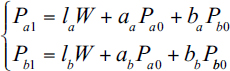
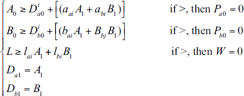
3. A very simple model will suffice for that purpose. Assume an economy with two goods only, a and b, each being both a consumption and a (circulating) capital good. The economy lasts two ‘years’ in all, t = 0 and t = 1, indicated by their initial moments 0 and 1. Production therefore occurs in a single cycle for t = 0, with all outputs becoming available at the end of that ‘year’ (a second production cycle in t = 1 would make no sense, because it is completed when the economy ceases to exist). As usual, all markets occur at ‘moment’ zero, so that the prices Pa1 and Pb1 of commodities a1 and b1 available for the year t = 1 are discounted to moment zero, when they are quoted together with the prices Pa0 and Pb0 of the spot commodities a0 and b0, and with the wage W.
We may at first suppose that one method only is known for producing each of the two commodities (this assumption will be abandoned in Section 1.5); la, aa, ba and lb, ab, bb are the corresponding production coefficients, which for simplicity we shall assume to be all strictly positive. The methods are of course assumed to be ‘viable’, i.e. capable of producing a surplus over the mere replacement of the means of production.
We shall then have the following equilibrium relations:
 |
(1.1e) |
| (1.2e) | |
 |
(1.3e) |
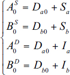
In system (E), equations (1.1e) are the usual competitive price relations for the products a1 and b1,11 while equation (1.2e) chooses b1 as the numéraire. The first two relations (1.3e), on the other hand, regard the supply of commodities a0 and b0, provided by endowments A0 and B0, and the demand for them, given by consumptions Da0 and Db0, plus investment (aaA1 + abB1) and (baA1 + bbB1), respectively; the third relation regards the demand and supply of labour, while the remaining two express the utilisation of the two outputs A1 and B1 for (only) the consumptions Da1, Db1.
System (E) thus has eight relations, only seven of which are independent, with seven unknowns: i.e. the four prices, the wage and the two outputs A1 and B1. Beyond the first test of consistency given by these numbers, the enquiry into the existence and character of the solutions of (E) will be part of the analysis we intend to conduct by means of the above-mentioned general equilibrium savings-supply and investment-demand schedules (see system (F) par. 7).
It may now be important to observe first that we have here simplified the system by ignoring the possibility of storing the two goods between t = 0 and t = 1, thus ‘transforming’ a0 into a1, and b0 into b1 — a simplification which does not affect the limited conclusions aimed at here, but the implications of which will be recalled below when necessary.12 It is this simplification which justifies the assumption that both commodities are produced, and that, therefore, relations (1.1e) hold with 2 a strict equality sign (cf. also Appendix II par. [iv]).
A second observation may be in order about system (E). The choice of b1 as numé raire in equation (1.2e) entails that the variables Pa0 and Pb0 emerge from (E) as the relative prices Pa0 /Pb1 and Pb0 /Pb1 which involve commodities of the two different dates, and which we shall accordingly call ‘intertemporal relative prices’. We shall distinguish them from ‘contemporary relative prices’, e.g. Pa0/Pb0, since we shall find that the properties of the two sets differ in important respects.13
4. We can now come to the decisions to save and to invest implied in system (E) for each of the two years’ life of the economy. Indeed, some readers might have been surprised by our reference in par. 3 to savings distinguished by year in a context of intertemporal equilibrium — where all contracts are made in an initial ‘moment’, and therefore all income is received and disposed off in that single ‘moment’; and furthermore it will be disposed in consumption only (if ‘final’ capital is zero). However, reflection shows that outputs, including of course capital goods, have to flow out year by year, and accordingly the incomes making up the prices of those outputs must also be distinguishable by year, together with their 20111 savings component.
The fact that, given the two years’ life of the economy, production only makes sense in t = 0, entails investment and savings will also only make sense for year t = 0. The aggregate decisions to invest I0 of that period are the value of two physical components Ia0 and Ib0, consisting of the parts of the two initial stocks A0 and B0 which are used as the means for the production of a1 and b1, and have already 6 appeared in the first two relations (1.3e). We thus have
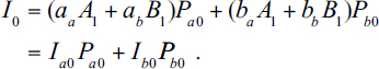 |
(1.4) |
Similarly gross savings S0 will be part of the social gross income Y014 of t = 0 — which, unlike the income Y1 of t = 1, will not be the counterpart of a social gross product, and will consist instead of the initial stocks, A0 and B0. Thus S0 will be expressed as the following difference between the gross income Y0 and the aggregate consumption G0 in year t = 0:
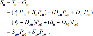 |
(1.5) |
where the physical components of the aggregate saving decisions S0 are distinguished by Sa0 and Sb0 and where the equilibrium magnitudes of system (E) imply Sa0 = Ia0, Sb0 = Ib0 and therefore I0 = S0.15
As for the year t = 1, we shall have
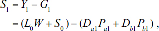
where (L0W + S0) is the value of the gross social product from the income side, and where, however, the last two equations (1.3e) stating that the entire output of t = 1 is consumed, entail I1 = 016 and S1 = 0.17
5. It may now be of interest to note how, in the individual ‘wealth equations’, relating to the entire lifetime of the economy, the savings of each year disappear (contributing perhaps to the misleading view that the problems raised by savings and investments disappear leaving place to a question ‘not any different from […] choosing commodities today’).18
The equation in question is in fact simply the sum of the yearly individual budget equations of the kind just seen, and in that sum the savings on the ‘expenditure side’ of the budget equation for any year t, reappear on the ‘income side’ for (t + 1), and must therefore cancel out with the latter (the exception being any savings of the final year of the economy which will of course be zero, if terminal capital is to be zero).
Thus, for example, the yearly budget equations of an individual in our two-year economy can be written as follows, where the small letters y, g, s stand for the individual’s income, consumption and gross savings for the respective year, and l0, a0, b0 stand for initial endowments:
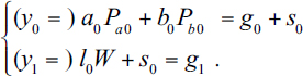 |
(1.5a) |
In summing equations (1.5a), the s0’s cancel out and we are left with
![]()
where the terms after the first equality sign constitute the ‘wealth equation’.
Non-zero gross savings and investments being possible in our model only for t = 0, we shall henceforth simplify our notation by dropping the zero deponent from the savings and investment variables.
1.3 The general-equilibrium schedules of savings-supply and investment-demand
6. Our task is now to bring out how the savings and investment decisions of equations (1.4) and (1.5) vary with prices and can accordingly affect the equilibria of the system. This is what will be done here by means of the two constructs mentioned already: ‘the general-equilibrium investment-demand schedule’ and ‘the general-equilibrium savings-supply schedule’.
The two schedules will be obtained from the relations of system (E) by (i) treating one of the two own rates of interest of period t = 0, say rb, as the independent variable;19 (ii) waiving the equality between I and S implied in (E).20 This requires first of all, the introduction of the definitory equation
 |
(1.6) |
The release of condition I = S, on the other hand, allows for either Sa ≠ Ia, or Sb ≠ Ib, or both, and therefore a difference between what we may now call the total demand of a0 given by A0D = Da0 + Ia (cf. the R.H.S. of the first of the relations (1.3e) in par. 3) and its total supply A0S = A0, which can also be expressed as A0S = Da0 + Sa (cf. equation (1.5), par. 4) — and similarly for the total demand and supply of b0.
7. The result is seen in system (F) below where,
1 the two unknowns A0D, B0D replace the data A0 and B0 in the relations (1.3e) which now, in their form (1.3f), with an equality sign only define the two total demands;
2 the data A0, B0, re-labelled as A0S, B0S, appear instead in the relation (1.5f) defining savings;
and where the unknowns I and S constitute the points of the two schedules corresponding to the given level of the independent variable rb:
 |
(1.1f) |
| (1.2f) | |
 |
(1.3f) |
| (1.4f) | |
| (1.5f) | |
 |
(1.6f) |
 |
(1.7f) |
All markets are here assumed to be in equilibrium except those of savings and investments, i.e. as we saw, the markets where saved and investible quantities of a0 and b0 are traded.21 System (F) in fact implies equilibrium
1 in the market for labour (see the respective relation in (1.3f));
2 in the markets for commodities a1 and b1 (see the last two equations in (1.3f));
3 in the markets of a0 and b0 for consumption (see the inclusion of Da0 and Db0 in equation (1.5f)).
However, if we exclude equation (1.7f) to be presently discussed, system (F) has eleven relations, ten of which are independent, containing eleven unknowns (the five prices; the two outputs A1, B1, the two aggregate quantities demanded B0D, A0D, and, finally, I and S).22 Were it not for equation (1.7f), system (F) would therefore possess the one degree of freedom which we could expect since, essentially, we replaced with the two new unknowns A0D and B0D, the single unknown Pb0 of (E) which becomes a given in (F) in the shape of the given rb = Pb0 − 1 of equation (1.6f).
Before discussing that degree of freedom, and its closure by means of (1.7f), we may, however, re-write the equations (1.3f), (1.4f) and (1.5f) in the more transparent form which we shall frequently use in what follows.
 |
(1.3f′) |
| (1.4f′) | |
| (1.5f′) |
8. In fact, the economic meaning of the degree of freedom we would have in (F) but for equation (1.7f) is quite simple. We have aggregated all decisions to invest into the single magnitude I, but nothing has been specified about the physical composition of the investment flows of Schedule I: this is what is done by means of equation (1.7f) which in fact fixes Ia/Ib jointly with Da0/Db0 since A0D/B0D is a weighted average of those two ratios.
That physical composition cannot, however, be specified arbitrarily. Our use of the I and S schedules in order to analyse the properties of system (E) imposes two requirements. The first and stricter requirement is that when S = I, the aggregate demands of a0 and b0 should also be equal to the respective supplies. And the same correspondence should hold for possible ‘extreme’ equilibria at the level rb min with S > I, or with W = 0 for S < I (see par. 14 below, points I and IV respectively, and Appendix I). This will in fact be the case when the proportion A0D/B0D in which the two commodities are there ‘demanded’ are the same as the proportion A0S/B0S in which they are supplied, as is imposed by equation (1.7f) (cf. parr. 15–16). The second, less strict, requirement is that the proportion A0D/B0D should reflect a non-unplausible out-of-equilibrium behaviour of the economy. And equation (1.7f) seems to provide a description of an out-of-equilibrium behaviour as plausible, it seems, as any equally general condition (cf. parr. 17–18).
9. There remains a rather technical point we need to consider in order to complete our account of system (F). It concerns the consistency of the system with the sum of the individual budget equations underlying it (Walras’s identity) and the often supposed impossibility of a disequilibrium confined to a single market, such as we have assumed in (F).23 However, that impossibility would follow only if the individuals could spend for the commodities available in t = 1 according to the total income which they would derive from selling exactly the quantities of a0 and b0 they wish to sell at the going prices (i.e. A0S/B0S in the aggregate, if we include in the demand the consumption by owners) and realise the corresponding savings for t = 0, but that is just what cannot happen when S ≠ I. When, on the other hand, the purchasing power for t = 1 originating from the savings S0 is appropriately ‘adjusted’ to what the going level I would allow them to sell of a0 and b0 — and this is what we have assumed in (F) — the contradiction disappears and system (F) is consistent.24
The ‘adjustment’ in expenditure we assume here, when compared with the more usual procedure of admitting disequilibrium in at least one further market, has the advantage of being compatible with a constancy in the employment of labour as rb, varies, thus providing a more transparent basis for deducing the shapes of the S and I schedules. It also allows for a simpler and perhaps better than any equally general representation of the out-of-equilibrium behaviour of the system, in the sense just mentioned that households failing to sell part of their A0S and B0S resources because of excess savings can hardly exert excess demand on the commodities of t = 1.25
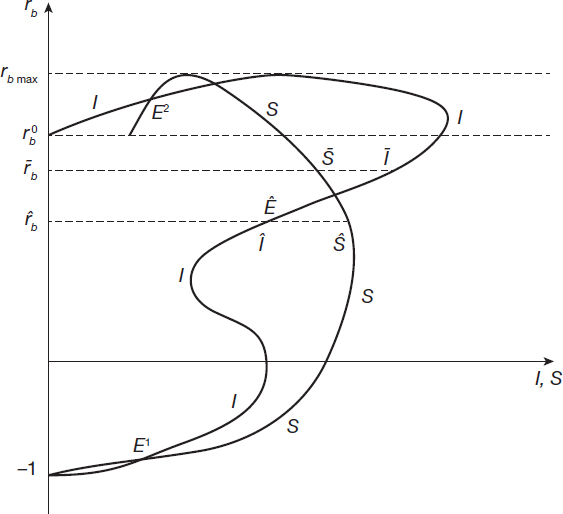
10. Some preliminary observations concerning our method of analysis may in fact be useful at this point. The general equilibrium nature of the two schedules and condition (1.7f) entail that any equilibrium in the market they represent is also an equilibrium of the system and that the converse is true (parr. 15–16). The properties of the general equilibrium relevant for its uniqueness and stability, and their dependence in particular on the circumstances of the savings and investment market then become visible in a form not unlike that of a partial equilibrium problem. It is in this way that in Sections 1.4–1.6 the two schedules will render visible a cause of multiple and unstable equilibria which does not appear to have yet been sufficiently analysed in the literature. That cause is the way in which investment changes as intertemporal prices change (see Figure 1.1).
Possibilities of non-uniqueness and instability of the equilibria have in fact been in the foreground of current general equilibrium literature. However, those possibilities seem to have been investigated in what we may describe as a mainly negative and economically unspecific way. The attention has been focused, that is, either on the impossibility of establishing uniqueness and stability under the more general premises of the theory, or on some sufficient, rather than necessary conditions for such properties.26 Similarly, the efforts seem to have been concentrated on systems of pure exchange, or of production without capital — this, despite the fact that the implications of reverse capital deepening and reswitching which had been pointed out for the traditional versions of neoclassical general equilibrium should have alerted scholars to the possible implications of those phenomena for intertemporal theory (cf. par. 2).
Thus, with regard to the causes of multiplicity and instability of the equilibria, recent literature does not seem to have added substantially to what, owing to a more simplified, but also better focussed analysis, had been known, since Walras, Marshall or Wicksell,27 about income effects and their causes. The paradox seems then to be that general conclusions about those properties that are at times presented as drastically negative for neoclassical theory28 have in effect favoured the comparatively comfortable, but unwarranted belief that the difficulties in question all have their origin in income effects — with which the theory has, after all, long managed to co-exist — and thus have had little dissuasive effect on the actual practice of the profession.29
11. Our general equilibrium demand and supply schedules may be seen as part of an attempt to remedy this situation by tackling again such central properties of the equilibria in the way Marshall, Walras or Wicksell approached them, that is by starting from specified economic conditions susceptible of causing the difficulties in order to arrive at their consequences for the equilibrium. This has led to an analysis of production with capital, and to focussing on the savings-investment market — on which reverse capital deepening impinges directly — in order to ascertain how those phenomena can affect the properties of a general intertemporal equilibrium (Figure 1.1).
A word of caution must now be added concerning our application of the method of general-equilibrium demand and supply schedules. Just because of its greater specificity, these tools of analysis bring to light questions which, apparently buried in the mathematical formalism previously used, require now30 definite answers. Where possible, those answers have been attempted here, however

provisionally. At other times the questions have been treated by referring to specific, more manageable sub-cases which do not however alter the generality of the negative results the paper is concerned with, since the sub-case is part of the general case.31 It may incidentally be stressed that when sub-cases have been resorted to, they have been specified so as to grant more favourable conditions to the theory. In particular, care has been taken to avoid mixing the cases of non-uniqueness, instability or zero factor prices emerging here, with the altogether different cases which might be due to income effects.
12. Passing now from the method to the content of our argument, the reader may ask why we have introduced the aggregate savings and aggregate investment of system (F) in order to discuss a system (E) which was in fact formulated independently of any such aggregates. The answer will of course have to come from what follows in this chapter. However, we have indicated already how the total demands of a0 and b0 which we find on the right-hand side of the first two relations in systems (1.3e), or (1.3f), are in fact made up of two quite heterogeneous elements each: the consumption demands Da0, Db0 (which we assumed to be always satisfied along the I and S schedules) and the investment demands I and Ib. Now, the investment demands are ruled by principles that are totally different from those which govern consumption demands: hunger can be satisfied by corn, and not by coal; but desire for future income, the motive of the demand for capital goods from savers, can surely be satisfied by tractors, as well as by looms or any of the thousands of other capital goods, whichever of them offers a higher rate of return. It can here be indifferently satisfied by a0 or b0 lent for production. In fact, as we shall see in par. 26, different capital goods are perfect substitutes for the savers.32
Now, in view of the different principles thus regulating investment demands as distinct from consumption demands, and in view above all of the perfect substitutability of heterogeneous capital goods for the saver, but of course not of consumption goods for the consumer — it does prima facie stand to reason that the separation of the two kinds of demand and, then, the aggregation of the capital goods demanded for investment, might lend transparency to the workings of the system.
13. In par. 8 we mentioned ‘stability’ among the properties of the equilibrium which might be inquired into by means of our two schedules. That implies that the schedules should be applied to discuss adjustments to the equilibrium. Although only hints of that analysis will be contained in the present chapter (parr. 17–18), we should perhaps clarify what can be meant by ‘adjustments’ and ‘stability’ here, in a context of dated equilibria.
In fact, as I have argued elsewhere (1976: 38), an analysis of stability, capable of fulfilling its traditional role of ensuring ‘correspondence’ between theoretical and observable magnitudes, has to be founded on the possibility of a sufficient repetition of transactions on the basis of approximately unchanged data. If a tendency to equilibrium could be established on that basis, it could also be generally supposed that disequilibrium deviations would tend to compensate each other, letting the equilibrium levels emerge as some average of observable levels, and be capable, therefore, of providing some guidance to reality. Essentially, the question in this respect would be to allow for a time setting in which
fitful and irregular causes in large measure efface one another’s influence so that…persistent causes dominate value completely.
(Marshall, 1949: p. 291)
That meaning of the positions of the economy to which theory refers its variables, and the corresponding notion of its stability, appear in fact to have been the unanimously accepted basis of economic analysis from Adam Smith, and before, until comparatively recent decades. At those earlier times, however, such a necessary repetition of markets on approximately unchanged data could be grounded in the conception of a normal position of the economy, a sufficient persistency of which was ensured by the uniform rate of return on the supply prices of the capital goods and by the corresponding adjusted composition of the capital endowment — which in neoclassical theory depends on the conception of the capital endowment as a single magnitude.33 If the abandonment of the corresponding notion of equilibrium (fundamentally different, recall, from that of ‘stationary’ or ‘steady states’) was by itself sufficient to undercut in fact the previous meaning of an analysis of stability, by imposing data too impermanent to allow for a sufficient repetition of markets, the ‘dating’ of the equilibria has jettisoned it even in principle by excluding repetition as such.34 This appears to leave in some obscurity the precise significance of present-day analyses of stability, quite independently of their negative results.
Our present critical purpose seems, however, to exempt us from entering further into the question and allows us to adopt the formal way out generally taken when the concern are still variables determinable by the equations of general equilibrium, and not the essentially indeterminable variables of a path-dependent equilibrium. This formal way out is, of course, that of ‘recontracting’, or of ‘tâtonnenment’, as it has come to be named with a misleading reference to Walras.35 In the modem fictitious theoretical world into which we shall enter by means of that assumption, the repetition of transactions — thus in fact admitted to be essential for an analysis of stability — is supposed to take place in some initial ‘moment’, or period before the actual time, measured out by ‘dated’ equilibria, has rendered such repetition impossible.
14. Though the model is simple, the discussion of system [F] and the determination of the schedules become complex as soon as we wish to go beyond the mere formal demonstration of the existence of solutions of system (F) — for which see the Mathematical Note at the end of the volume (p. 469) — and we attempt to gain an understanding of their properties and economic meaning. We have accordingly placed that discussion in an Appendix and shall here confine ourselves to listing the conclusions we shall use in the rest of the chapter, references being given to the Appendix for the supporting argument.
I. When we suppose, as is done above, that neither commodity can be stored, the economically meaningful interval of rb extends from rbmin = −1, for Pb0/Pb1 = 0 (Appendix I par. [1]) to a level rbmax, the highest among those for which W = 0 (see point IV below).
II. Changes in the intertemporal relative price rb = [(Pb0/Pb1) − 1] need not affect in one direction rather than the other total relative demands of the two contemporary commodities a0 and b0, i.e. the ratio (Da0 + Ia)/(Db0 + Ib), and therefore the relative contemporary price Pa0/Pb0 necessary to satisfy equation (1.7f). Making then the further reasonable supposition that such a contemporary relative price will not be much affected by changes in rb, we assume that the intertemporal price Pa0/Pb1 moves in the same direction as Pb0/Pb1 and hence rb in the interval rbmin < rb < rb+ in which W > 0. This suffices to ensure a unique solution in an interval rbmin < rb< rb0 where rb0 ≤ rb+ is, as we shall see under point IV below, the minimum level for which we find W = 0 (Appendix I, parr. [5]–[7]).
III. Two other important consequences follow from that assumption. The first is that the monotonic relation between Pa0/Pb1 and Pb0/Pb1 entails a decreasing relation between W and the intertemporal price Pb0/Pb1 and hence rb over the whole interval rbmin < rb < rb+, along what we shall call ‘the main branch’ of the relation between rb and the unknowns in (F), in particular between rb and I and S. That ‘branch’ is of course where, as we saw under point II, we have unique solutions, but only up to rb0 and not for rb0 ≤ rb ≤ rb+ where a continuum of positions for W = 0 will exist (see point IV below). The second important consequence of the monotonic direct relation between the intertemporal prices Pa0/Pb1 and Pb0/Pb1 is that ra will move in the same direction as rb allowing us to refer unambiguously to a rise or fall of the own interest rates (Appendix I parr. [8]–[9]).
IV. Should labour continue to be supplied at W = 0 — as would generally be necessary for ensuring the continuity of the functions and the existence of solutions of system (E) (ibid. par. [10]) — then at that zero level of W we shall find a con tinuum of solutions of (F) for levels LD of labour demanded in the interval 0 ≤ LD ≤ LS, and for the corresponding levels of rb in the interval rb0 ≤ rb+ ≤ rbmax where, with rb0 as the minimum such level, rbmax ≥ rb0 is the maximum one (ibid. par. [6]: see also Figure (1.2)).
V. The minimum level rbmin = −1 corresponding to the intertemporal price Pb0/Pb1 = 0 does not entail, as one would perhaps expect, that b0 is a free com modity so that, for example, also Pb0/Pa0 = 0 . On the contrary, there are reasons which force us to admit that, as Pb0/Pb1 → 0, the contemporary relative price Pb0/Pa0 will generally tend to a positive and finite level, with all commodities available in t = 0 having zero price in terms of all commodities available in t = 1 (ibid., parr. [7] and [12]).
VI. As for the shape of the two schedules (see Figure 1.1) what we can say generally is that: (i) the choice of b1 as our numéraire entails, as just said, that for rb = rbmin = −1 both Pa0 and Pb0 are zero, so that both the S and I schedules intersect the vertical axes at rb = −1; (ii) as we saw under point III a ‘main branch’ of the S and I schedules will exist in the interval rbmin ≤ rb ≤ rb+: along it W will decrease from Wmax for r = rbmin down to zero for rb+; (iii) the two schedules will then continue beyond rb+ in order to represent the continuum of positions indicated under point IV above, with the I schedule finally reaching the vertical axis with LD = 0 (ibid. par. [14]); (iv) it does not seem however that anything general can be said about the overall shape of the schedules in the intermediate interval 0 ≤ rb ≤ rb0 except for the single-valued character of the schedules seen under point II and the bias towards rising S and I schedules due to our choice of b1 as numéraire, and therefore of Pa0 and Pb0 rising as rb rises (a bias which is of course innocuous as far as the properties of the equilibria are concerned, which only depend on the ratio S/I at each level of rb); (v) in particular, the impossibility of supposing a necessarily falling I schedule is not however due to that bias. Nor is it due to the fact that alternative techniques have not yet been considered: possibilities of substitution between labour and means of production are already present in the system because of consumer choice between a1 and b1. The essential reason why a falling I schedule cannot be assumed will be seen below (par. 19) and is the same as for the phenomenon of reverse capital deepening, familiar from the traditional analysis. No confusion should in fact be caused by the presence of two consumption goods which could conceivably engender a rising I schedule because of income effects: as we make clear by one of the assumptions on which our argument is based (Assumption (IIIa), ibid. par. [5]), our conclusions are independent of any income effects.
1.4 The representation of the intertemporal system
15. What we must now see, therefore, is how the two schedules can aid our understanding of the behaviour of system (E). In this and the next paragraph we shall see how the schedules can represent the equilibria of the system and then, in the following two, we shall consider the information they can provide on out-of-equilibrium behaviour.
A ‘position’ (F) of the system (i.e. the solution of (F) for a particular value of rb) will also be an equilibrium (i.e. a solution of E) when the first two relations in (1.3e) of par. 3, concerning the aggregate demand and supplies of a0 and b0 happen to be satisfied: all other relations of (E) are in fact already present in (F). Leaving aside at first the case of ‘extreme’ equilibria occurring, that is, for rbmin or for W = 0, it can be asserted that when the system is in equilibrium the two schedules S and I intersect, and that the converse is also true.
As for the first proposition, when rb is in that intermediate interval, or also in the upper interval rb+≥ rb≥ rb0 along the ‘main branch’ of the S and I functions (point III in par. 14), and Pa0, Pb0 are accordingly strictly positive, any solution of (E) entails that the first two relations in (1.3e) of par. 3 above are satisfied with an equality sign,36 i.e.
| (1.3a) |
and hence (see relations (1.3f′) in par. 7)
| (1.3a) |
and
| (1.3b) |
The general equilibrium of the system thus entails an intersection of the two schedules.
As for the converse proposition, when we have an intersection of the schedules in that same interval (see Figure 1.1, par. 11), equation (1.3b) is satisfied and therefore, after adding Da0Pa0 + Db0Pb0 to both sides, we obtain
| (1.3c) |
Indicating then, by the constant γ, the common value or the ratios appearing on the two sides of equation (1.7f), we may write equation (1.3c) above as follows:
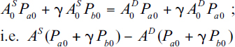 |
(1.3d) |
from which A0S = A0 D and hence, from equation (1.3c), B0S = B0D, thus fulfilling all relations (1.3e) in system (E), and ensuring that we are in a general equilibrium position.
16. Turning now to the representation of possible ‘extreme’ equilibria of the system, we may note that equilibria in the upper interval rb0 ≤ rb ≤ rbmax (see Figure 1.2) will also be shown by intersections of the two schedules, but the converse proposition will not be true. Since different (F) positions may correspond to the same level of rb, an intersection between I and S may occur in that interval at a point representing an (F) position on the I schedule, and a different one on the S schedule. The intersections representing equilibria have then to be traced by checking whether the I and S points of the intersection pertain to the same (F) position. This will be possible in the diagram because, starting, for example, from points like I+ and S+ (see Figure 1.2), the two schedules will go through exactly the same values of rb in exactly the same sequence: ‘couples’ of I and S points corresponding to the same (F) position can therefore easily be singled out.37 The reasoning conducted in the preceding paragraph will then apply to those points of intersections which represent the same (F) position on both schedules.
As we proceed to rbmin, at the opposite extreme, although the zero intertemporal prices Pa0, Pb0 yield S = I = 0, we shall generally have definite non-zero physical

Figure 1.2 The upper reaches I+I0 and S+S0 of the I and S schedules representing positions (F) for W = 0 characterised by different levels of labour employment and therefore of the investment required to equip them
quantities Ia, Ib, Sa, Sb (par. [13] in Appendix I). We need first of all to note here that the assumption about both goods being scarce for consumption in t = 0 as well as in t = 1 (see Assumption (ii) in par. [3] of Appendix I) entails that the position (F) for rb = −1 is the one characterised by the ‘collective’ zero intertemporal price of all commodities available in t = 0 relative to those of t = 1, which we mentioned under point VI of par. 14 and discussed in parr. [7] and [12] of Appendix I.
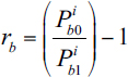
Now, that (F) position is an equilibrium when, as rb → rbmin, Sb > Ib. At that position savings would generally exceed investment when expressed in contemporary prices by means of either a0 or b0. Then, by a reasoning analogous to the one conducted in par. 15 for equations (1.3c) and (1.3d) we could in fact conclude S > I; Sb > Ib and therefore we have an ‘extreme equilibrium’ with A0S > A0D; B0S > B0D. When however S < I as rb → rbmin no equilibrium will generally exist at rbmin.38
17. While thus representing the equilibria of the system, the two schedules can, as we said, provide elements for a discussion of its out-of-equilibrium behaviour. Suppose first an (F) position for rb = rb′ in the interval rbmin < rb′ < rb0 such that S′ > I′ (see Figure 1.1, par. 11). As we just saw, the inequality S > I entails A0S > A0D and B0S > B0D. It would then seem natural to suppose an ‘initial’ reaction in the markets for a0 and b0, more directly affected by the disequilibrium, which would occur before adjustments can take place in connected markets: in our case under the reasonable assumption of excess supply for both commodities, that ‘initial’ competitive reaction could only be a fall of intertemporal prices Pa0/Pb1 and Pb0/Pb1. However, the connected markets will then tend to adjust, so that we may envisage an out-of-equilibrium behaviour in the recontracting dominated by movements centring on the two general equilibrium schedules. In this respect equation (1.7f), assuming a proportionate change of the algebraic excess demands of a0 and b0, seems to be as reasonable an assumption as can be made at a general level: it may indeed be taken to represent a condition of ‘even flexibility’ of the price system, in the sense of allowing for the excess demands of a0 and b0 to change in the same proportion. Our critical aim strengthens on the other hand the legitimacy of assuming that the dominant out-of-equilibrium movement will be along the schedules: if deficiencies of the demand and supply apparatus result under that assumption, they would seem to be all the more plausible when obstacles to the adjustments to equilibrium are also considered in the connected markets, which the schedules assume instead to be broadly kept in equilibrium.
Then, as we start moving along the schedules, the ‘initial’ fall of both Pa0/Pb1 and Pa0/Pb0 in response to the assumed excess savings will result in a movement downward along the schedules with a fall of both own rates ra and rb (see point III in par. 14). This result can indeed be taken to be general — largely independent, that is, of our assumption about the monotonic rise of Pa0/Pb1 with Pb0/Pb1 (cf. point II in par. 14, and par. [8] in Appendix I).39
Similarly to what could be argued in any partial equilibrium use of the schedules — we have then elements for arguing a tendency e.g. toward equilibrium EIII in Figure 1.1 of par. 11, where the I schedule cuts the S schedule from above and where therefore any given initial position in the interval rbIII < rb< rbIV, rb can be expected to fall, and to rise for any rb in rbII < rb < rbIII. A tendency away from equilibrium can instead be argued when, as we move from left to right, I cuts S from below (see EII and EIV in Figure 1.1).40
18. As we turn to ‘extreme’ values of rb, we may note that if we happened to have S > I in the proximity of rbmin = −1, the fall of rb, which we can assume in the presence of S > I, would imply competitive recontracting to tend to the equilibrium with the zero intertemporal (but not contemporary) prices of both a0 and b0 we saw in par. 16.41
As we could expect, some novel problems are met when we shift our attention to the upper extreme for rb0 ≤ rb ≤ rbmax. We may leave aside the ‘main branch’ of the S and I schedules (where with L = LD and W > 0 we have all the conditions for the out-of-equilibrium behaviour considered in par. 17). In all other (F) positions of that interval, we shall have excess supply of labour with L > LD and a zero wage. The I schedule will tend to finally extend leftward so as to reach the vertical axis for the (F) position corresponding to LD = 0 (cf. par. [14] in Appendix I) and, as we just saw in par.16, any equilibrium will be shown by the two schedules intersecting, and intersecting for the same (F) position.
Outside any such equilibria, if in the given position (F) we have I< S (see e.g. points I″ and S″ in Figure 1.2) it would be natural to suppose that the excess savings, i.e. the excess supply of a0 and b0, will cause the ‘initial’ fall of both Pa0/Pb1 and Pb0/Pb1 we admitted for intermediate levels of rb.
However with W = 0 and the available excess supply of labour making it possible to expand outputs, that temporary ‘initial’ fall of the prices of a0 and b0, relative to those of their outputs a1 and b1 would make it profitable for entrepreneurs to raise outputs, and as adjustments occur we would tend to move along the I schedule towards the right in the direction of an increase of the labour employment LD and therefore of the investment required to equip that labour. Prices Pa0 and Pb0 will have to move in the opposite direction and so may therefore do ra and rb. Unless an equilibrium were to be met in the process, that increase of LD would continue until full labour employment is reached in position (F+) for rb = rb+. Excess savings and the consequent persisting ‘initial’ fall of Pa0/Pb1 and Pb0/Pb1 would then result in a positive wage W, and a fall of rb: the (F) positions would become those already discussed in par. 17, characterised by W > 0.
In the case in which, in that same upper interval of rb and for W = 0, we instead had I > S in the (F) position — as exemplified by points I′ and S′ in Figure 1.2, for the same level rb″ of rb of the just discussed position (F) with excess savings — then, an opposite process of decreases of employment LD and investment would have to be expected. It would lead leftwards along the I schedule to an equilibrium which would then have to exist. As we just recalled, investment I has in fact to change continuously down to zero, while S also changes continuously, though generally without reaching zero. Then, with I starting to the right of S and having to pass finally to its left while going through exactly the same levels of rb, it is inevitable that the two schedules will cross — as exemplified by E2 to the left of the points I′ and S′ in Figure 1.2.
1.5 Alternative techniques and the investment demand
19. System (F), like system (E) which generates it, still rests on the assumption that only one method of production is available for each commodity. It is time to drop that assumption and consider the existence of several alternative methods for each commodity, all sharing the properties we mentioned in par. 3. We may call a set of ‘methods of production’, one for the commodity in question and one for each of its (direct and indirect) means of production, ‘the system of production’ or ‘technique of production’ of the commodity. Here, the ‘technique’ or ‘system’ of production of the commodity will accordingly include two ‘methods of production’, one for the commodity and one for the other commodity as means of production of the former. Thus one ‘technique’ for producing a, will also be a ‘technique’ for producing b, and we may therefore refer to techniques i = 1,…, n without mentioning the commodity they refer to.
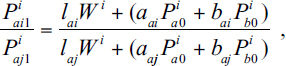
Despite our assumption that all alternative methods of production require the same three factors, there is no assurance that marginal products, even of the discontinuous kind, will exist.42 For the determination of the method that would be the cheapest at current prices and would therefore be chosen by competitive entrepreneurs, we must therefore resort to the more general approach we find in Sraffa’s Production of Commodities: namely, comparing the expenses for producing the commodity by the alternative methods. However, at each level of rb the comparison can only be done in terms of prices Pa0i, Pb0i and the wage Wi holding for the particular technique i ‘in use’ — meaning here by ‘in use’ that the technique is the one whose adoption we assume to be generally planned at the stage reached by the recontracting.43 Maximisation of entrepreneurial profits will then entail that the recontracting proceeds to any method for each commodity which happens to be cheaper at those prices.
A question which is well known from the ‘traditional’, non-intertemporal assumptions then arises, about whether the order of the alternative methods of production of the commodity as to cheapness, might not itself change with the technique ‘in use’: with the possibility of either endless switching between techniques, or of the technique finally adopted depending on the one initially ‘in use’. Our critical intent, however, will again allow us to grant the assumptions most favourable to the theory criticised and therefore to assume what has been demonstrated to be true under the traditional assumptions: that the order of cheapness of an alternative method is the same, whichever the technique in (planned) use at the given level of rb.44 We can thus suppose that entrepreneurs’ choice will always arrive at one and the same method(s) for each of the two commodities, so that at any given rb the cheapest technique(s) or ‘system(s) of production’ can be uniquely determined, together with the corresponding series of the prices, the outputs, and the I and S quantities, where the plurals above take care of the possible co-existence at some rb of two (or more) methods for the same commodity and hence of the technique(s) differing from i by the method of that single commodity which will then entail the same wage and prices for the given level of rb.
20. We can therefore proceed to reporting below the family (Fi) of systems of equations defining the two schedules under the assumption of a multiplicity of techniques of production j = 1, 2, 3… . Each member of that family is a system of equations like (F) defined in par. 6, but applied now to the technique i which happens to be the one no dearer than any other at the given level of rb. Thus, to any level rb in its relevant interval there will correspond a system (Fi) containing, as well as the relations (F) pertaining to the technique i adopted, as many quadruplets of relations, (8fi) and (9fi), as there are alternative ‘techniques’ or ‘systems of production’ j ≠ i. The first two equations (i.e. 8fi) reckon the production expenses of a1 and b1 with the respective methods j. The second couple of relations, namely (9fi), states that no method j for producing each of the two commodities is cheaper than the method pertaining to the technique i ‘in use’.45
 |
(1.1fi) |
| (1.2fi) | |
 |
(1.3fi) |
| (1.4fi) | |
| (1.5fi) | |
 |
(1.6fi) |
 |
(1.7fi) |
 |
(1.8fi) |
| (1.9fi) |
where i at the exponent indicates that the variable in question is calculated under the assumption that technique i is being planned for use at the given rb, whereas j at the deponent indicates the alternative technique to which there pertains the variable in question, coefficient of production or price based on such coefficients (no deponent has been given to the same variables pertaining to technique i). The equality signs in (1.9fi) take care of the possible co-existence between technique i and other techniques for same levels of rb, when the equality sign will apply to both the relations (1.9fi).
Correspondingly, also system (E), determining the equilibrium of the system, should now be written in the form of the following family of systems (Ei) allowing for alternative techniques:
 |
(1.1ei) |
| (1.2ei) | |
 |
(1.3ei) |
 |
(1.8ei) |
| (1.9ei) |
where, as for (E) in par. 3, the relations corresponding to equations (1.4fi), (1.5fi), (1.6fi) and (1.7fi) do not need to appear, S = I being implied in (Ei).
21. The main question which the existence of alternative methods of production raises for us here is the changes in the investment requirements I due to changes in the cheapest technique as rb varies. We might perhaps expect that owing to those changes (as well as to those of the relative outputs A1/B1 already determined in system F) the schedule I would generally show a negative slope. However, such an expectation has no better foundation for the present investment-demand schedule than it had for the capital-demand schedule in the ‘traditional’ setting.
A simple line of reasoning seems sufficient to show this. As has been pointed out,46 the roots of reverse capital deepening, as well as those of the re-switching of techniques, lie in the effect of changes in distribution (rate of profits) upon the relative value of the alternative sets of capital goods required by the processes of production which are being compared — whether such processes are alternative methods of production for the same consumption good, or the methods for two different consumption goods. In the traditional, non-intertemporal setting, it is the changing relative value of such two sets of capital goods that can make a more ‘capital-intensive’ technique become more profitable, or a more capital-intensive consumption good fall in price, as the interest rate rises. And it is that same change in the relative value of the alternative sets of capital goods that can bring about ‘re-switching’ among alternative techniques. Now, the same variability of the relative value of alternative sets of capital goods is clearly present in an intertemporal setting.
To see the thing in more definite terms, let us consider first the case of alternative techniques as distinct from that of competing consumption goods. From equations (8fi) and (9fi) we may see how, at the given level of rb, the choice between the cheapest technique i and any other alternative technique j differing, say, by the method of production of a alone, hinges on the following relative costs of the two methods:
 |
(1.10) |
the method of technique i for a1 being more profitable than the j one at the given rb when Pai1i/Paj1j < 1. Defining now
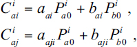
where the Cai’s are the respective capital expenses estimated at the given level of rband for i prices. We may then write the relative production expenses (1.10) of the two methods as follows:
 |
(1.10a) |
With (Caii /Iai) and (Caji /Iaj) as the respective ratios of capital to labour in the (direct) production of a1, we then have
 |
(1.10b) |
Assume now, without loss of generality, that Caii/Iai > Caji /Iaj . Should the Cai’s be measured so that they are independent of changes in W, clearly Pai1/Paj1 could only fall as W rises (and rb falls: point III, par. 14). Any changes of method could only be in favour of the more “capital intensive” one (from j to i in our case). Since however the Cai’s and therefore the key ratio Caii/Caij are not so independent, the rise of W (fall of rb) need not entail the fall of Pai1i/Pai1j we might have expected: a sufficient rise of Caii/Caji may well make Pai1i/Paj1i rise, and not fall as Wi rises. This means that the rise of W may well result in the less capital-intensive method j becoming the more profitable one of the two, and therefore being adopted.
The same change of Caii/Caji in the relative value of the sets of capital goods of the two alternative processes of production may entail, as can be shown by replacing Paj1i with Pbi1i, that the less ‘capital-intensive’ consumption good b1 may become cheaper relative to a1 as W rises (rb falls) so that regular substitution in consumption has “perverse” effects on factor demands. Hence the freedom with which we were able to draw the shape of the I schedule in our Figures 1.1, 1.2 or 1.3.47
1.6 Some conclusions
22. We can now use the schedules to see some properties of a general inter temporal equilibrium and thereby how ‘capital’ as a single ‘quantity’ enters intertemporal equilibrium. The question may usefully be approached by showing how misleading is the widespread idea is that savings and investment in an inter temporal equilibrium raise no more problems than do relative demands for contem porary commodities and can therefore be subsumed under a single theory of consumer choice.48
It is of course true that if we assume no capital to be left at the final date, the (gross) savings at t must consist of demand for consumer goods at future dates (t + τ), at the expense of demand for the same or other consumer goods at t. It is then equally true that any excess of saving decisions over investment decisions at t must necessarily take the form of an excess supply of consumer goods at t, and an excess demand for them at future dates. Thus, imagine that initial recontracting had brought the economy to the position (![]() ) of quantities and prices which the system (Fi) associates with the interest rate
) of quantities and prices which the system (Fi) associates with the interest rate ![]() b (see Figure 1.3), and suppose that (
b (see Figure 1.3), and suppose that (![]() ) would coincide with an equilibrium (Ê) except for a positive excess of savings Δ
) would coincide with an equilibrium (Ê) except for a positive excess of savings Δ![]() = (
= (![]() − Î), (
− Î), (![]() ) and (Î) being estimated at the prices of (
) and (Î) being estimated at the prices of (![]() ).
).
From the households budget equations in (Fi) for ![]() b we obtain
b we obtain
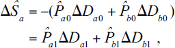 |
(1.5b) |
where the ΔD’s indicate the differences in the respective quantities demanded between positions ![]() and Ê (where savings would have been equal to Î); which, for simplicity, we have supposed to be both negative in t = 0 and positive in t= 1.49 Undoubtedly, equation (1.5b) looks similar to that holding in the case of
and Ê (where savings would have been equal to Î); which, for simplicity, we have supposed to be both negative in t = 0 and positive in t= 1.49 Undoubtedly, equation (1.5b) looks similar to that holding in the case of
contemporary commodities, should (![]() ) have failed to be an equilibrium simply because of an excess demand of b0 relative to a0, giving
) have failed to be an equilibrium simply because of an excess demand of b0 relative to a0, giving
| (1.5c) |
23. However, the analogy between equations (1.5b) and (1.5c) remains at the surface of the two phenomena and hides a basic difference between them which emerges as soon as we consider the adjustments which should lead to a new equilibrium and therefore the forces warranting it in the two cases. That basic difference can be best brought out if, for a moment, we extend our two-year model to the three years (−1), (0), (1), with the commodities a0 and b0 accordingly coming from production in t = −1 by means of L−1 labour and A−1s, B−1s initial stocks.
Now for the contemporary commodities of equation (1.5c), the question of achieving a neighbouring equilibrium will be the comparatively simple one of shift ing the labour and means of production of (t − 1) freed by (−ΔDa0) to producing ΔDb0 and no obvious obstacle stands in the way of achieving that as a consequence of the competitive rise of Pb0/Pa0, which would plausibly follow from initial competitive bidding in the situation.
The position is entirely different in the intertemporal (savings/investment) case of equation (1.5b). Obviously, it will not be possible to shift the labour and the means of production of period t = −1, set free by the reduced consumption of t = 0, to directly producing the increments ΔDa1, ΔDb1 of equation (1.5b): the labour and means of production of t = −1 are not those of t = 0, which can directly produce ΔDa1 and ΔDb1. Even less will it be possible to devote to the direct production of ΔDa1 and ΔDb1 any of the labour and means of production of t = 0, which could directly produce them, but unlike those of t = −1 are assumed to be already fully employed. No competitive rise of Pb1/Pb0 plausibly following from the relative rise of consumption demands in t = 1 can achieve either of those two feats.
How, then, can we raise the t= 1 outputs and consumptions and, moreover, do so at the expense of the consumptions of t = 0, as required by the excess savings of equation (1.5b)? The answer clearly remains that of traditional, non-inter temporal theory. This change of relative outputs over time can only be achieved by raising the gross productivity of the already fully employed labour L0, by means of an increase, in some sense, of the quantity of means of production cooperating with it. It is a question, that is, of producing in t = −1 quantities ΔIa and ΔIb while decreasing production by quantities ΔDa0 and ΔDb0, and then using the increments of investment with the constant quantity of labour L0 to produce increments ΔDa1 and ΔDb1 of consumption. But, and here comes the essential point, those increments of investment can only be motivated by the rise of the intertemporal prices of a1 and b1, relative to b0 and a0, i.e. by the fall of the interest rates: no question of the increments of investment being caused directly by the additional consumptions ΔDa1, ΔDb1 entailed in the savings of equation (1.5b) — contrary to the case for the contemporary consumptions of equation (1.5c).
The idea that savings and investment in intertemporal equilibrium cause no more problems than relative demands for (contemporary) commodities should rather be turned upside down into the one that intertemporal equilibrium raises the problem of savings and investment in basically the same terms as traditional equilibrium does.
24. The problem then is of course that what the capital controversies taught about ‘capital reversing’ and ‘re-switching’ in traditional equilibrium — and has been confirmed for the present context in par. 19 — entails that the rise of the intertemporal prices Pi,t+1/Pi,t (i = a, b), i.e. a fall of the own rates of interest ri,t might fail to provide the entrepreneurs with a motive for that increase ‘in some sense’ of Ii which is required for the intertemporal adjustments in consumption. The result might then be the striking one that, however small the initial excess savings, the theory could force us to admit movement to an equilibrium with drastic changes in wages and prices (cf. in Figure 1.3 above, the equilibrium E1 to which there would be a tendency starting from the position ![]() for
for ![]() b in our original two-year model). Further, if the position
b in our original two-year model). Further, if the position ![]() with excess savings happened to be that for
with excess savings happened to be that for ![]() b < rb″ in Figure 1.1 (par. II, p. 125) the theory would force us to admit a tendency to negative interest rates if not to the zero intertemporal prices Pa0 and Pb0 for our economy with non-storable goods.50 And as indicated in par. [12] of Appendix I such zero intertemporal prices far from being a result of satiety, would mean that the attempt of some individuals to take care of even more acute scarcities in t = 1 runs counter to the inability of the market forces, as envisaged in the theory, to transfer consumption from t = 0 to t= 1.51
b < rb″ in Figure 1.1 (par. II, p. 125) the theory would force us to admit a tendency to negative interest rates if not to the zero intertemporal prices Pa0 and Pb0 for our economy with non-storable goods.50 And as indicated in par. [12] of Appendix I such zero intertemporal prices far from being a result of satiety, would mean that the attempt of some individuals to take care of even more acute scarcities in t = 1 runs counter to the inability of the market forces, as envisaged in the theory, to transfer consumption from t = 0 to t= 1.51
Alternatively we might find an equilibrium in which it is W0 which has to become zero,52 with the attending labour unemployment, when the initial con tracting had brought to a level rb for which ![]() >
> ![]() (see in Figure 1.3), the equilibrium E2 to which there would be a tendency when the economy happened to start from rb =
(see in Figure 1.3), the equilibrium E2 to which there would be a tendency when the economy happened to start from rb = ![]() b.
b.
25. The above difference between the cases of contemporary and intertemporal consumptions allows us to begin seeing how the concept of a quantity of capital enters intertemporal general equilibrium. What we have analysed in parr. 23–24 is no less and no more than the process of substitution between labour and “capital”, the single factor, which underlies the determination of distribution between wages and profits in the traditional versions of the theory, exemplified by our reference to Wicksell’s Lectures in par. 2. The process was there viewed as involving the entire capital and labour endowments, whereas here it has been dealt with from the viewpoint of flows and not funds. But if ‘capital’ was what Wicksell and traditional theorists dealt with for their determination of wages, interest and prices, then — as indeed we foresaw in par. 2 — ‘capital’ is also what we have dealt with when studying the forces that should correct a surplus or deficit of savings over investment, thus determining the prices, in particular the own interest rates, of our simple intertemporal equilibrium and their properties.
Thus we duly found there the central relevance of an inverse relation between the own interest rates and the ‘amount’ of means of production, i.e. of capital per worker in the economy: as we saw, only if that inverse relation holds, can entrepreneurs operate adjustments towards plausible equilibria in intertemporal consumptions. And that inverse relation is of course the same which was required to ensure adjustments to plausible equilibria in the market for ‘capital’ and the other factors in the traditional version of the theory. Also the consequences of the impossibility of measuring that ‘amount’, i.e. ‘capital’, in terms independent of distribution are then essentially the same as in the traditional versions of the theory. Also the consequences of the impossibility of measuring that ‘amount’, i.e. ‘capital’, in terms independent of distribution are then essentially the same as in the traditional versions of the theory. As we recalled in par. 21, that impossibility undermines the inverse relation between interest rates and capital intensity and therefore the uniqueness, stability and overall plausibility of the resulting equilibria.54
No important difference is on the other hand made by the fact that in the intertemporal versions the inverse relation concerns a set of own rates (intertemporal relative prices) rather than the traditional single interest rate. A tendency of the own rates to move in the same direction can be argued and, more importantly, any contrasting movements among the own rates can be seen to be due to intratemporal phenomena hardly relevant for intertemporal adjustments (cf. parr. [7]–[9] in Appendix I).
26. This re-emergence of the neoclassical need for a ‘quantity of capital’ in intertemporal equilibria goes back ultimately to the basic fact that the demand for capital goods obeys principles altogether different from those governing the demand for consumption goods (par. 12). Whereas the latter comes from preferences that are specific to the goods demanded, the former results from savers’ preferences that are non-specific to the individual capital goods, and are only specific with regard to the aggregates of them. This is lucidly expressed by Walras when he introduces savings in his general equilibrium as the demand of the particular commodity which he calls ‘perpetual future income’,55 with a price of its own which is the reciprocal of the (effective) interest rate. That of course means that, in proportion to their value, capital goods are perfect substitutes for the saver as means of transferring income in time.56
The question of a ‘quantity of capital’ in neoclassical theory is indeed no more than an application of Jevons’s ‘law of indifference’ concerning the single competitive price and hence a single magnitude by which we must refer to any commodity which individuals, in this case wealth holders, treat as homogeneous. Just as one chooses according to the principle of the minimum price between alternative sources of, e.g. ‘corn’ — so one chooses between the alternative sources of ‘perpetual net income’, the different capital goods, according to the minimum price of such ‘future income’ — i.e. the maximum of the effective net rates of return. Capital goods are no more distinct commodities for savers than physically homogeneous ‘corn’ from different farms is for its consumers.
In the case of capital goods, this basic fact is however obscured by a second fact, which mixes the market for the single commodity ‘future income’ with a second layer of markets and where, furthermore, a quite different kind of substitutability emerges among capital goods. Unlike homogeneous corn where the allocation of consumers’ demand among different merchants or farms is theoretically uninteresting beyond the application of Jevons’s law of the tendency to a single price, the allocation of the demand for future income among potential sources of supply involves nothing less than the entire theory of production — in order to determine the rentals of the several capital goods and their ratio to the respective supply price. This gives central visibility to that allocation and substitutability in production which, however, is ultimately no more relevant for an explanation of the rate of interest, or system of own rates of interest (intertemporal relative prices), than the analogous allocation of the aggregate demand for corn among the several farmers is for the explanation of the price of corn. Just as it is only the aggregate demand and the supply of corn that is relevant for determining the price of corn, so it is only the demand and supply of aggregates of capital goods that is relevant for the determination of the rates of interest.
27. The presence at some stage of the theory of a quantity representing aggregates of capital goods is therefore as inevitable for the neoclassical determination of prices on the basis of the demand and supply decisions of individuals,57 as is the presence of the quantity of each consumption good. Individual demand and supply decisions about capital goods are ultimately taken in terms of that ‘quantity’ just as the similar decisions about corn consumption are taken in terms of the quantity of corn. It is on a single commodity ‘capital’ and not on individual capital goods that savers’ preferences operate, whether in the traditional ‘fund’ context, or in the intertemporal ‘flow’ context.
The traditional versions of the theory, with their equilibrium condition of a uniform effective net rate of return on the supply prices of the capital goods, entailed already taking care of that single commodity at the level of the endowment of factors,58 and those authors did so by expressing the endowment of capital directly as a single ‘quantity of capital’, its allocation in a capital-goods vector being then an unknown of the system. The abandonment of that traditional long-period notion of the equilibrium — not to be confused, recall, with a stationary or steady state59 — and of its specific condition of a uniform effective rate on capital good supply prices has meant getting rid of the single commodity ‘perpetual net income’ and of its bearer, ‘homogeneous capital’, but only at the cost of assuming away, at the level of the factor endowments, the perfect substitutability of capital goods for the saver, and Jevons’s indifference law with it: no surprise, then, for the methodological problems which are raised by today’s pure theory.60
However, those high methodological costs may have been borne in vain. They have been borne, that is, for what may turn out to have been getting rid of the obviously inconsistent notion of a ‘quantity of capital’ at the level of the demands and supplies of the immediately visible factors of production, and therefore at the level of the endowments, in order to have it re-enter the theory at the less immediately visible but theoretically equivalent level of investment-demand and savings-supply.
Appendix I: The determination of the I and S schedules
[1] In par. 7 of the text1 we had a first check of the consistency of system (F) by counting independent relations and unknowns. The existence of economically meaningful solutions for the unknown prices and quantities of (F) in the economically relevant interval of rb, rbmin ≤ rb ≤ rbmax to be presently specified, is demonstrated in the Mathematical Note at the end of this volume (p. 469). However, an intuitive account of the demonstration is necessary for a better understanding of the argument which we have conducted, and of the assumptions we have introduced.
We start by noting the lower limit of the relevant interval of values of rb. Due to our assumption that no storage is possible for either commodity,2 the ‘intertemporal price’ Pb0/Pb1 can fall to zero and equation (1.6f) of par. 7 will accordingly give
| (1.6b) |
The specification of the upper limits of rb where W = 0 will, on the other hand, require a better acquaintance with the properties of system (F) and we shall come to it in par. [6] below. 4
[2] As we proceed to the intermediate range of rb, equations (1.2f) and (1.6f) of system (F) in par. 7 of the text allow us to write the second price equation (1.1f) as follows:
| (1.1a) |
where, having used equation (1.2f), Pa0 is now in effect the intertemporal price Pa0/Pb1 as, of course, is Pb0 = (1+rb).
Two implications of equation (1.1a) are of interest here.
(a) It is only for bb(1+rb) ≤ 1, i.e. for rb ≤ (1−bb)/bb that we may have non-negative values of both W and Pa0. Considering also rbmin from equation (1.6b), we may therefore begin to restrict our attention to the interval
 |
(1.6c) |
of our independent variable, where (1−bb), and hence (1−bb)/bb, are evidently positive whenever the method of production of b is viable (par. 3 in the text).
(b) Equation (1.1a) above will then entail that for any rb in the interval (1.6c), non-negative levels of W require Pa0 to stay in the interval
 |
(1.1b) |
Given, then, rb and Pa0 in the respective intervals (1.6c), (1.1b), equation (1.1a) will determine the corresponding non-negative level of W. Consequently the first of equations (1.1f) determines Pa1. Thus the entire series of prices and the wage will be uniquely determined by equations (1.1f), (1.2f) and (1.6f), once Pa0 is given, besides rb.
To that unique series of prices and the wage, there will correspond the quantities demanded expressed by the functions Da0, Db0, Da1, Db1. The amount of total savings S in equation (1.5f) with its physical components Sa, Sb of (1.5f) will then be determined as well. The methods of production of the two commodities, being given, the same will be the case for the amount of investment I of equation (1.4f) and its physical components Ia, Ib. Such quantities need be neither single-valued, nor continuous functions of Pa0.3 It will however follow common practice and not be unduly restrictive to make the following assumption:
Assumption (i) Given rb in the interval (1.6c), the quantities demanded Da0, Db0, Da1, Db1, and hence the aggregate quantities demanded A0D and B0D are single-valued, continuous functions of Pa0 in the interval (1.1b).4
[3] Thus, then, given a level of rb in the relevant interval, any level of Pa0 in the interval (1.1b) will entail a ratio δ = A0D/B0D which will generally differ from the ratio δ = A0S/B0S, equality with which is imposed by equation (1.7f). As we then change Pa0 in the interval (1.1b), there are three possibilities (cf. Figure 1.4 in the Mathematical Note to this chapter).
(a) At one or more levels of Pa0, δ = γ. Equation (1.7f) will be satisfied and we shall have a solution of (F) for each of those values of Pa0.
(b) Over the entire interval (1.1b) of Pa0, δ < γ. This will mean that at the given level of rb it will be impossible to use a0 in as high a proportion to b0 as that in which we find the two commodities in the endowment. This means then that a0 would be a free good in an equilibrium occurring at that level of rb, when, that is, A0D = A0S.
(c) Finally, over the entire relevant interval of Pa0, we shall have δ > γ. This is the case symmetrical to (b), in which b0 cannot be used in as high a proportion to a0 as B0S/A0S (in as low a proportion as AS/BS) and b0 would be a free good in an equilibrium occurring at that particular level of rb, which would then have to be rb = −1, because of Pb0 = 0.
Cases (b) and (c) would exclude an economic solution of system (F) as formulated in the text, with equalities in the first two relations (1.3f), but the simple economic rationale of the cases, i.e. the non-scarcity of either a0, or b0 when equality between demand and supply were to be achieved for the other, indicates that a solution could be ensured by a slight formal modification of (F).5 However, that would complicate the exposition and risk obscuring the main points we wish to bring out, which are altogether independent of that kind of excess supplies. We shall therefore leave aside cases (b) and (c), as on the other hand we implied already by assuming two (scarce) goods in our model, for period t = 0, no less than for t = 1. We may therefore render explicit the following assumption:
Assumption (ii) In the interval rbmin ≤ rb ≤ rbmax, in which W = 0, and for rbmax to be defined below (par. 6), the commodities a0 and b0 can be used in the proportion A0S/B0S in which they appear in the endowment.
We may then conclude that, for any level of rb in the interval between rbmin and the level rbmax to be defined, at least one level of Pa0 will exist satisfying equation (1.7f), and thus solving system (F).
[4] The key role of the price Pa0 in the solution of (F) at any relevant level of rb calls for a specification, since there are two aspects of that price which play a different role in system (F): an ‘intertemporal’ aspect and a ‘contemporary’ one.
Having been expressed in terms of the numéraire b1 of equation (1.2f), Pa0 possesses an ‘intertemporal’ aspect, the one which we have chosen here to measure by rb (i.e. Pb0/Pb1), the independent variable of our system (F). Pa0 however also possesses a ‘contemporary’ aspect, which may be expressed by π = Pa0/Pb0, a new variable. Indeed:
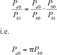 |
(1.2f′) |
In par. [3], with rb a given, variations of Pa0 were in fact variations only of the contemporary relative price p. The intertemporal role of Pa0 will instead be prominent when considering the joint variation of Pa0 and Pb0 with rb, as we shall presently do in Assumption (iii) (see also par. [7]).
[5] The generally made Assumption (i), and the confirmation of the two scarce-good nature of our model by means of Assumption (ii), are sufficient to ensure the existence of a solution for (F), but not its uniqueness: income effects may cause the same ratio A0S/B0S to occur for more than one value of π = Pa0/Pb0, at a given level of rb. We may however make the following assumption:
Assumption (iii) The value of π = Pa0/Pb0 satisfying equation (1.7f) together with the remainder of system (F) is unique for each level of rb in the interval rbmin < rb < rb0, where rb0 is the lowest level of rbfor which W = 0. Further, Pa0 will be a continuous increasing function of Pb0 i.e. of rb, in the interval rbmin < rb < rb+, where rb+ ≥ rb0 is the level at which that joint rise of Pa0 and Pb0 will have to cease, having brought to W = 0 in equation (1.1a) (par. [2] above).
By excluding more than one level of p for which the ratio of the total demands (Da0+Ia)/(Db0+Ib) of a0 and b0 can satisfy equation (1.7f), the first part of Assumption (iii) excludes income effects which in t = 0 might make the ratio A0D/B0D decrease through decreases in the consumption ratio Da0/Db0, as Pa0/Pb0 falls; it also excludes similar effects in t = 1 causing Da1/Db1 to change so as to make Ia/Ib fall rather then rise as π = Pa0/Pb0 falls.6 Since here we wish to exclude income effects, we may proceed and make the following:
Assumption (iii(a)) A monotonic inverse relation is assumed between Da0/Db0 and Pa0/Pb0 as well as between Da1/Db1 and Pa1/Pb1.
Assumption (iii(a)) only has the purpose of clarifying that the results which we shall reach as to multiplicity and instability are altogether independent of income effects. The assumption will have no consequences on our argument beyond those following from the weaker Assumption (iii).
On the other hand, as we shall see in par. [7], the direct relation between the two intertemporal relative prices Pa0/Pb1 and Pb0/ Pb1, postulated in the second part of Assumption (iii), amounts to simply supposing that the change in the intertemporal price rb will cause no large dislocation in the contemporary relative demand Da0/Db0 and Ia /Ib, so that the relative contemporary price π need not undergo large changes in order to continue and satisfy (equation 1.7f).
We shall see in par. [8] some important implications of Assumption (iii) with respect to the relations between W and rb, and between the ‘own rates’ ra and rb. But before coming to that, we must deal with the upper limit of rb and thereby clarify the relation between the three levels rb0, rb+, rbmax which Assumptions (ii) and (iii) have already associated with W = 0.
[6] We saw that the monotonic rising relation between Pa0 and rb (i.e. Pb0) of Assumption (iii) comes to an end when, for rb+ = Pb0+ − 1, W becomes zero in equation (1.1a). This zero wage will then permit labour unemployment in (F), and allow for a continuum of solutions of (F), one for each level of labour ‘demanded’ LD in the interval 0 ≤ LD ≤ L. In the resulting continuum of solutions of (F), rb can fall from rb+ down to the mentioned minimum level rb0 and/or rise up to a highest level rbmax, giving rb0 ≤ rb+ ≤ rbmax.7 It also follows that in such a sub-interval of rb, Pa0 and all remaining unknowns in [F] will no longer need be single-valued functions of rb (see Figure 1.2, in the text, par. 24). Since, on the other hand, using (1.2f′) of par. [4] equation (1.1a) of par. [2] becomes
| (1.1a) |
π = Pa0/Pb0 will have to change along that continuum of (F) positions, in a direction opposite to that in which rb and hence Pb0 vary.8 Thus for rb0 ≤ rb ≤ rb+, the increasing relation of Assumption (iii) between Pa0 and Pb0 (i.e. rb) will only hold for the values of Pa0 corresponding to what we shall call the ‘main branch’ of the function linking rb with π and the remaining unknowns in (F) — the only branch, that is, in which W > 0.
[7] We may now come to what turns out to be perhaps the key relationship in the system, the one already considered in Assumption (iii) between the contemporary relative price π = Pa0/Pb0, and the intertemporal relative prices, represented here by rb.
Thus, let us drop equation (1.7f) from system (F) for a moment, and see the likely effect on A0D/B0D of a fall of Pa0, which happened to be in strict proportion to that of Pb0.9 By thus keeping constant π while rb falls we aim to distinguish between the ‘intertemporal’ effects of that fall and the side-effects if any, that it may have on the relative demands of a0 and b0 — and hence, once equation (1.7f) is re-introduced, on the contemporary relative prices π = Pa0/Pb0 and Pa1/Pb1, as well as on the other own rate of interest, ra (par. [8]).
Now, the proportionate fall of Pa0/Pb1 and Pb0/Pb1 might be thought to affect the decisions to save and invest in some definite direction, but no general reason appears to exist why the ratios Da0/Db0 or Ia /Ib, and therefore the ratio A0D/B0D = (Da0 + Ia)/(Db0 + Ib), should be affected in one direction rather than the other. It follows that, quite independently of any uncertainty due to the income effects which we chose to rule out by Assumption (iii(a)) in par. [4], we could not expect any definite sign in the change of π necessary to keep A0D/B0D at the A0S/B0S level imposed by equation (1.7f): π may, that is, move either way, or even alternate the signs of the change as rb falls; and the same will be true for the other contemporary relative price Pa1/Pb1, controlled by price equations (1.1f). Therefore, unless the fall of rb causes pronounced dislocations of relative demands in t = 0, a tendency can be supposed for the contemporary price π not to change drastically as rb falls and, therefore, for the intertemporal price Pa0/Pb1 to follow the other intertemporal price Pb0/Pb1 (i.e. rb) in its fall. This tendency of the two ‘inter temporal’ prices to fall or rise together is at the basis of our Assumption (iii).
An important and perhaps surprising implication of what we have just said should now be noted for future reference. We saw that no reason exists why as rb falls towards rbmin, the relative contemporary price π = Pb0/Pa0 should move in one direction rather than the other. However, the own interest rb falling towards the minimum level of (−1) holding when the commodities are not storable is in fact the intertemporal price Pb0/Pb1 of b0, falling towards zero. It therefore appears that in system (F), the assumption of a zero level of the intertemporal price Pb0/Pb1 of b0 does not entail a zero level of its contemporary price Pb0/Pa0, contrary to what we would expect from a commodity which is becoming ‘free’ in the generally accepted sense — when a tendency to zero of the price of the commodity in terms of one scarce commodity (b1 in this case) would entail a tendency to zero of its price in terms of all other scarce commodities (like a0 here) whether of the same, or of another, date. We shall return on this basic point in par. [12].
[8] After seeing the grounds on which Assumption (iii) rests we may now turn to two important implications of that assumption. The first is that, as shown by equation (1.1a) of par. [2] the monotonic direct relation between Pa0 (i.e. Pa0/Pb1), and rb (i.e. Pb0/Pb1) entails a monotonic inverse relation between rb and W in the interval between rbmin and rb0. The same is true for any level in the upper interval rb0 ≤ rb ≤ rb+, limitedly, however, to the ‘main branch’ of the functions linking rb to p and the other unknowns of the system (par. 6).
The second implication of Assumption (iii) is that the monotonic increasing relation between the intertemporal prices Pa and Pb there specified, also entails a monotonic increasing relation between ra and rb so that over that interval the two own rates of interest will always move in the same direction.10
[9] It is indeed time for some more general considerations on the relationship just referred to between own rates of interest. The considerations will refer to our simple model, but appear susceptible of generalisation.
There seems indeed to be no reason why ra should always move in the same direction as rb when the latter changes in system (F). The relation between the two rates ensured by arbitrage is given by:
 |
(1.6a) |
where the factor within square brackets shows, as we would expect, that the proportion between the two rates of t = 0, established by arbitrage, compensates the disadvantage which those, who lend in terms of the commodity whose relative price falls between time t = 0 and time t = 1, would otherwise have: thus if it is a that falls, the factor in question is larger than 1, and ra is correspondingly larger than rb, and vice versa.
The two rates might therefore move in an opposite direction over a limited interval of rb11 but only if the change in rb were to modify considerably the variation in the relative price of the two commodities over the year: where the stress falls on ‘modify’ rather than ‘variation’, since a constancy in the price variation would allow the two rates to move, not only in the same direction, but also in strict proportion. However, the variation in question is governed by the technical conditions of production expressed in price equations (1.1f) and its change is not therefore likely to be large unless the change in rb affects very strongly the ratios between the three factor prices Pa0, Pb0, W and, besides, large differences exist in the pro portion in which the three factors are used in producing the two goods.
[10] We have so far been mainly concerned with the determination of the two schedules at intermediate levels of rb. Completion of the analogous determination at the ‘extreme’ values of rbmin = −1, and rb0 ≤ rb ≤ rbmax, for W = 0, raises some additional problems connected with the zero levels of W or Pb0 which those extremes imply.
We may turn first to the case of W = 0 along the corresponding upper range of rb (par. [6]), and have a closer look at the supply of labour in that range. It has often been noted that there is no reason why, as the wage approaches zero, the supply of labour should also approach zero. If wages are the only income available to the worker for survival, the supply of labour can easily be imagined to increase, rather than decrease, as the wage gets close to zero (a quarter pound of daily bread is better than nothing).12 The situation only changes when the wage actually reaches zero, and supplying labour no longer makes any sense for the worker. It would thus seem reasonable to envisage a discontinuity in the supply of labour at a zero wage or close to it, where a jump to zero would presumably occur from the high level to which the supply might tend as the wage tends to zero.
Such a discontinuity would, however, have the undesirable consequence of eliminating the certainty of the existence of at least one economically significant solution to a system of general equilibrium: in particular the system would no longer admit the zero wage solutions should the supply of labour happen to exceed demand at all strictly positive wages. We have therefore followed what seems to be generally supposed: i.e. a continuity of the supply of productive resources even at zero prices for their services and, therefore, that the quantity of labour made available at that price is the limit to which that quantity tends as the wage tends to zero,13 which in the system (F) is the given supply L. This assumption — which we have in fact used already, when referring to a continuum with different levels of labour employment at a zero wage in the range rb0 < rb < rbmax (par. 6) — and the irrational behaviour it would entail, should however be kept in mind when, in what follows, the shape of the I schedule will show the possibility of equilibria in the interval rb0 ≤ rb ≤ rbmax.
[11] As we proceed now to the analogous question concerning savings, i.e. the supply of a0 and b0 as capital goods, it is similarly possible to envisage a state of acute scarcity for individuals whose only way to survive in t = 1 are stocks of (non-storable) a0 and b0. Savings may then well increase in physical terms as both intertemporal prices Pb0/Pb1 and Pa0/Pb1 tend to zero (on that joint tendency to zero of all intertemporal prices for commodities available in t = 0 cf. par. [12]), with savers discontinuously annulling their useless savings as those prices actually reach zero, and rb = ra = −1.14 We shall however assume continuity in the supplies Sa and Sb of a0 and b0 as capital goods, so as to ensure the existence of at least one general equilibrium for the system. We shall therefore find at zero inter temporal prices, the levels of physical savings to which Sa and Sb tend as rb tends to (−1).
[12] As a second preliminary to considering more closely the determination of the extreme points of the I and S schedules, we must now examine the meaning of the zero price Pb0/Pb1 we assume when referring to the point in the schedules for rbmin = −1. This zero intertemporal price presents an interest which goes beyond its direct importance, confined as that is in system (F), to the case in which no commodity in the economy can be stored. As we noted in par. 7, where we first came across it, that zero price does not designate b0 as a free commodity in the generally accepted sense of having a zero price also in terms of any other scarce commodity besides b1. On the contrary we saw that there is no reason why b0’s contemporary price π = Pb0/Pa0 should be zero when Pb0/Pb1 is such.
The two kinds of prices, contemporary and intertemporal, have in fact two quite different meanings. The intertemporal price Pb0/Pb1 expresses the conditions at which the commodity can be transferred over time — and thus reflects merely the scarcity or abundance of savings relative to investment needs. The contemporary price π = Pb0/Pa0 reflects instead the scarcity of b0 relative to a0 in t = 0, and by setting rb = −1 we did not assume anything in particular about it. This contemporary relative scarcity is largely dependent on the endowments A0S and B0S, which remain exactly the same all along the I and S schedules and up to rbmax.
Indeed our Assumption (ii) in par. 2, that a0 and b0 can always be used in the given proportion A0S/B0S, has excluded the possibility of either b0 or a0 having a zero contemporary relative price whether at rbmin or at any other level of rb. And what we just saw in par. 11 entails that both b0 and a0 might become increasingly scarce for consumption in t = 0, as rb approaches its minimum level, with the corresponding definite scarcity of b0 relative to a0, expressed by π = Pb0/Pa0. What is assumed not to be scarce the moment in which we give the value of (−1) to our independent variable rb is only the purchasing power which people seek to transfer from t = 0 to t = 1, relative to the only possibility to collectively do so in that economy: lending capital goods a0 and b0 to producers, who transform them into a1 and b1: but for that to happen a0 and b0 must be demanded for production and can therefore be in excess supply, independently of their scarcity in consumption in t = 0.
This nature of the zero price of b0 at rb = −1 comes more fully into light when we observe that arbitrage will then entail zero intertemporal prices of all commodities dated t = 0 in terms of any other dated t = 1. Were it not so anybody wishing to exchange b0 for b1 could do so via a1 (if Pa0/Pa1 > 0),15 or by first getting a0 and then b1, and this either directly (if Pa0/Pb1 > 0), or again through a1 (if Pa0/Pa1 > 0).
[13] We are now finally able to complete our discussion of the solutions of (F) at the lower and upper extremes of the possible levels of rb. With respect to rbmin = −1, we know that, given the continuity assumed in par. 11 for the supply of physical savings, solutions of (F) will exist there, no less than for the remaining interval rbmin < rb ≤ rbmax.16 We are therefore legitimised to extend to that point Assumption (iii) about the uniqueness of the solution of (F).
The peculiarity of the diagrammatic representation of this point is that the zero price we find there for both commodities a0 and b0, of which I and S physically consist, will make the two schedules converge to zero as rb reaches (−1) (see Figure 1.1, in the text, par. 11). The positive, finite contemporary relative price of the two commodities available in t = 0 (par. 7 and 12) entails however that, should we choose to measure S and I by taking a0 or b0 as the numéraire, we would find there two non-zero separate points S and I, with Sa, Sb being both smaller or both larger than Ia, Ib, the sign of the inequality being the one indicated by the relation between S and I as rb approaches rbmin sufficiently (cf. par. 15 in the main text).
[14] As we proceed to the determination of the I and S points of the schedules at the opposite extreme, we find the continuum of (F) positions we outlined in par. [6]. That continuum, we said, will correspond to levels of labour employment LD between zero and L, with the corresponding changes of the investment required to equip that variable amount of labour.17
We may look at the continuum by starting at rb = rb+, where W reaches zero after falling monotonically from its maximum level as rb rises from rbmin up to rb0, and then along the ‘main branch’ of the function linking I, S and the other unknowns of (F) with rb (see Assumption (iii), par. [5]). Beyond rb+, the I schedule will however sooner or later turn left as it will have to extend to touch the vertical axis as the investment demand falls to zero together with the amount of labour LD to be equipped by means of that investment (see Figure 1.2 in par. 16 of the text). Thus, starting from the value rb+, the schedule I may either rise or fall as it moves right or left, to finally reach the vertical axis on the left, having its highest and lowest points at, respectively, rbmax and rb0, each or both of which may or may not coincide with rb+.18
The levels of S will similarly change as rb varies in that interval, and the schedule may also extend either right or left as it rises or falls together with the I schedule, starting from point S+ for rb+. No reason however exists why it should tend to zero as LD tends to zero (see again Figure 1.2 in the text):19 at the corresponding points, savings remain those effected out of the endowments A0D and B0D: wages being zero, the different levels of labour employment do not affect the income out of which savings are decided.
Appendix II: Two notes on Hahn on ‘the neo-Ricardians’
[A] Two meanings of the uniform rate of return on capital and some mathematical flaws in Hahn’s (1982) argument
[i] What follows is not a belated commentary on, or an answer to, Hahn’s (1982) article on the so-called ‘neo-Ricardians’. That misleading article had essentially two aims: the first was to claim that Sraffa and his ‘followers’ were only concerned with a ‘Special case’ of neoclassical theory; the second was to answer their critique, centred on the notion of a ‘quantity of capital’, by contending that the notion plays no role in neoclassical theory.
Now, the first claim has been answered time ago by explaining that in the classical theory of Smith and Ricardo which Sraffa aimed to revive, the idea of a distribution of the social product based on the substitutability of ‘productive factors’ and therefore on the determining role of ‘factor endowments’ is absent; so that Sraffa’s contribution cannot be based on the assumption of the capital endowments of Hahn’s ‘Special neoclassical case’.1
As for the second contention the answer is in the main text above, where it is argued in detail how a ‘quantity of capital’ is implied, together with its deficiencies, in an intertemporal equilibrium. It is also contended there that a reference to that ‘quantity’ in neoclassical theory is rendered ultimately inevitable by the fact that capital goods are for savers perfectly substitutable means of acquiring future income and savers’ decisions are accordingly taken with respect to that single ‘quantity’ (parr. 26–27 in the text).
[ii] What follows in this Appendix is therefore confined to two specific points intended to clarify some misunderstandings that have seriously marred the ‘capital controversies’ so far. The first is a widespread confusion between two quite different kinds of uniform rate of return on capital: a uniformity of own commodity interest rates, and that of effective rates of return on the supply prices of the capital goods. This confusion, causing the flaws we shall see in Hahn’s (1982) mathematical argument, is an expression, I shall argue, of the obscuration of the change which has occurred in the notions of equilibrium during the last few decades and of its deeper causes: the change, that is, sometimes perceived as the ‘Formalist revolution’ in neoclassical theory.2
The second point, considered in Section B, regards instead a peculiarity implicit in the new notions of equilibrium, which Hahn again expresses in a particularly candid way when assuredly denying that the ‘quantity of capital’ has any relevance in neoclassical pure theory. The peculiarity consists, essentially, of regarding physical compositions of the capital endowment the economy moves away from, as equivalent, in defining non-stationary equilibria, with physical compositions the economy tends to.
[iii] In Hahn (1982) a key role is played by the distinction between a ‘General’ neoclassical case and a ‘Special’ one, where the latter is characterised by a uniformity of the rate of return on capital. The distinction echoes in fact one drawn by critics early in the capital controversies (par. [vii]), between the contemporary versions of neo-classical theory and the traditional ones based, as the latter were, on the above condition of a uniform effective rate of return on the supply prices of capital goods, and on the resulting ‘adjusted’ physical composition of the ‘capital stock’ (n. 2 in the text).
Hahn’s model is the one we adopted for our chapter, and his ‘General’ neoclassical case coincides with our system [E]3 but for two elements. The first is the exclusion of the inequality signs, and associated zero prices, from the first three relations of our system [1.3e]4 (par. 3 in the text), regarding factor demands and supplies. The missing inequality signs rule out, besides the possibility that one of the factors be non-scarce in the generally accepted sense, the less obvious possibility of ‘extreme equilibria’ arising from excess savings (point III in par. 14 of text).
[iv] Of more interest to us here is however a second shortcoming of Hahn’s formalisation. It is his supposition that ‘both goods are produced’ (ibid., 364), which he does not motivate, as we did (par. 3 of the text), by the assumption that the two goods are non-storable: in fact the whole issue of the storability of commodities, hardly separable from that of an intertemporal equilibrium, is absent in Hahn (1982). Now, in that unspecified form, Hahn’s assumption is in conflict with the fact that the two goods are also capital goods, and for durable or storable capital goods, the possibility of demand prices below supply prices, and therefore temporary non-production of them, is the logical entailment of a system, like Hahn’s, based on a given physical composition of the initial capital endowments5 (e.g. the so-called ‘Hahn problem’ about adjustments to equilibria rests entirely on some capital goods not being produced, and their prices being therefore free to move below the respective supply prices so as to adjust to price expectations). The result is that when applied to ordinary and therefore durable, or storable capital goods, Hahn’s ‘General neoclassical case’ falls into an overdeterminacy which, curiously enough, is a neat replica in terms of present-day intertemporal general equilibria of the overdeterminacy to be found in Walras’s originary general equilibrium system.
The question here is ultimately that of the uniform effective rate of return on the supply prices of the capital goods. Demand prices below the respective supply prices for capital goods offering a potentially lower rate of return, is indeed the way in which arbitrage achieves a uniformity of returns on the demand prices of the capital goods. The moment in which such prices are equalised with the respective supply prices — in which, that is, production of all capital goods is assumed6 — also is the moment in which we are introducing in the equations the traditional equilibrium condition of the uniformity of rates of return on the supply prices, postulated by Walras in common with all his contemporaries and successors up to recent decades. But in Walras that traditional condition was in conflict with a capital endowment given in its physical composition, and not as the abstract ‘quantity of capital’, susceptible of assuming any physical form, of his contemporaries and successors — thus causing what I have elsewhere referred to as ‘Walras’s inconsistency’.7
Now, in Hahn’s intertemporal context, with price changes considered in the equilibrium equations, a uniform effective rate of return necessarily takes the form of rates of interest which differ according to the commodity in which the loan is expressed (like ra ≠ rb in our chapter). This effectively uniform rate of interest, and therefore of return on the demand prices of capital goods, is introduced in the equations when we refer to n−1 discounted prices for n dated commodities, thus implying arbitrage through triangular intertemporal exchanges. It becomes therefore a uniform rate of return on the supply prices of the capital goods, the moment in which these goods are assumed to be produced and, accordingly, their prices are equalised with the supply prices. And this is just what is done by Hahn in his ‘General’ case, when he assumes that both goods are produced. The condition thus introduced cannot however be generally satisfied in his context, any more than it could in Walras’s original system, since the physical composition of the capital endowment is as given in Hahn as it was in Walras.
This flaw of Hahn’s treatment, we said, is curious. Walras’s inconsistency had been acknowledged by Hahn in e.g. an earlier (1975) paper of his and indeed, as we shall see in par. [vii], is the very one he intends to show to affect the ‘Special case’ and to have been overcome in the ‘General case’, which we now see to be instead affected by it (the ‘Special case’ being affected by an overdeterminacy of quite different origin, cf. par. [v]). The contradiction is strictly connected with the confusion between two kinds of uniformity of rates of return we mentioned at the beginning, and to which we can now turn.
[v] The confusion emerges as we proceed from Hahn’s ‘General’ neoclassical case to his ‘Special’ case, and note a third flaw in Hahn’s mathematical argument. He obtains the ‘Special’ case by adding to the relations of the General case that of a uniformity of the two own interest rates:
 |
[I] |
i.e. the condition of a constancy Pa0/Pb0 = Pa1/Pb1 of the relative price of the goods over the two periods (see equation [21] in Hahn, 1982: 364).
Now, uniformity (I) of the own commodity interest rates is quite a different matter from the uniformity of the effective rates of return on the supply prices of the capital goods referred to by the critics, to whom Hahn is there intending to answer (par. [vii]). However, he analyses the former as if it were the latter: in particular, he incorrectly attributes the overdeterminacy of his ‘Special’ case to the cause pointed out by critics for Walras’s overdeterminacy, i.e. the given proportions between the stocks of the several capital goods in the endowment.8
That Hahn’s interpretation of his own ‘Special’ case is incorrect can, on the other hand, be easily seen as soon as we extend from two to three years the life of the economy of his model (clearly, Hahn does not intend his distinction between ‘General’ and ‘Special’ neoclassical cases to be valid only for a two-year economy). We would then have two additional unknown prices Pa2, Pb2, but three new equations: the two additional price relations of type (1e) of par. 3 in the text, and the equation Pa1/Pa2 = Pb1/Pb2 relating to the uniformity of the own rates in t = 1. Thus the total of excess equations in the ‘Special’ case now adds up to two, against which the single additional unknown B0 or A0/B0 proposed by Hahn is of no avail. Indeed the physical composition of the initial capital stock has little to do with a constancy of relative prices, i.e. with the kind of uniformity of returns Hahn states in equation (I) for his ‘Special’ case.9 This uniformity would depend, if anything, on the size rather than the physical composition of the capital endowment: it would be the size of that endowment, relative to that of labour and other original factors, that might ensure the incomes, and therefore the savings, of a stationary or steady-growth economy with its constant relative prices.10
[vi] In fact both in his interpretation of the ‘Special’ neoclassical case, and in his assumption that all capital goods are produced (par. [iii]), Hahn takes as one:
(a) the uniformity of the own commodity rates of interest of equation (I), due to a constancy of relative prices over time;
(b) the traditional uniformity of the effective rate of return on the supply prices of the capital goods, the result of an adjusted physical composition of the capital stock (par. [i]),
where uniformity (b) is independent of (a) since, as shown for Hahn’s ‘General’ case (par. [iv]), it is quite compatible with changes in equilibrium relative prices over time, and therefore with the divergent own commodity rates ruled out by uniformity (a).
And Hahn takes (a) as if it were (b) not only when, as we saw, he ascribes the overdeterminacy caused by equation (I) and uniformity (a) to the proportions between the two stocks as if it were due to (b): he does so also when the traditional uniformity (b), being unaccompanied by (a), unlike what happened in the old theorists referred to by the critics (par. [vii]), is unwittingly introduced in a ‘General case’ intended to show those critics how one can do without that very traditional uniformity (b).
We may also note here incidentally that Hahn appears to misinterpret the divergence of own commodity rates of interest when he writes: ‘The crudest empirical observations will convince one that there is no unique rate of profits to be observed in the economy: Do we conclude from that that competition is functioning badly? Answer: No. Consult any general equilibrium text’ (1975: 361), thus apparently referring to divergences of own commodity rates. However, what empirical observation can reveal is divergent profit rates for different businesses, compared therefore in terms of money or some other common numéraire. But then, that divergence has nothing to do with divergences between own commodity rates, which would show by reckoning in different numéraires the same rate of profits (when, of course, the relative prices of those numéraires change over the year).
[vii] Unambiguous confirmation of the Hahn (1982) confusion about uniform rates, as well as of the intent we attributed in par. [iii] to his (1982) distinction between ‘General’ and ‘Special’ neoclassical cases, can in fact be obtained from the already quoted earlier (1975) paper of Hahn. He referred there to results advanced early in the capital controversies by the critics, who had pointed out how the contemporary attempt to surmount the inconsistency of the notion of a ‘quantity of capital’ by taking the capital endowment as a given physical vector entailed falling into the alternative inconsistency of Walras’s originary general equilibrium. This was the case unless uniformity (b) was dropped, together with the entire traditional notion of equilibrium, as is done in contemporary pure theory — thus undermining, it was further argued by those critics, the persistency of the equilibria necessary for a correspondence between theoretical and observable variables.11
Accordingly, in (1975), Hahn begins by reporting statements by Harcourt (1975) to the effect that in the ‘Walrasian model’ it is not possible to have a ‘theory of the rate of profits’ [read: to determine a uniform rate of return on capital of type (b) above] and that
to get a uniform rate of profit Wicksell (and others) had to work with Robinsonian leets [homogeneous capital].
(Hahn, 1975: 360–361)
To this Hahn objects that the ‘Walrasian model’ can deal with ‘the uniform rate of profit’ by treating it as just ‘an extremely specialised case’ (Hahn, ibid.).
The passage is of some interest in itself because Hahn acknowledges there those early critical results of the capital controversies, and in particular: (i) the inconsistency between ‘uniform rate of profit’ and ‘Walrasian model’ and, there-fore, (ii) the role of ‘Robinsonian leets’ (homogeneous capital) for ‘Wicksell and others’ in allowing for a uniform rate of profit. However, surprisingly enough, those two points are not mentioned in the (1982) paper, apparently devoted to answering the ‘neo-Ricardian’ critique on capital of which they evidently were central elements.12
What is of specific interest to us now is however the confirmation which the (1975) article gives of the confusion about uniformity of rates of return, and of the intent of the ‘Special’ neoclassical case. With respect to the first point Hahn describes as follows the ‘specialisation’ of the ‘Walrasian model’ yielding Wicksell’s ‘uniform rate of profit’:
General Equilibrium Theory is general and so we can discuss the equilibrium of an economy whatever its initial conditions, e.g. outfit of goods inherited from the past. For most such specifications it will not be the case that the equilibrium equilibrium price of a good for future delivery in terms of the same good for for current delivery will be the same for all goods.
(360, our italics)
But the uniformity of the rate of profits of ‘Wicksell (and others)’, i.e. uniformity (b) above, is quite different from ‘the equilibrium price of a good for future delivery in terms of the same good for current delivery [being] the same for all goods’, quite different, that is, from the uniformity (a) of own rates to which Hahn refers here.
(We may incidentally note how the above straight identification of Wicksell’s uniform rate of profits with a uniformity of own rates of interest which is simply a constancy of relative prices, provides the key to what probably misled Hahn and other authors into confusing the two uniformities. In Wicksell, as in Walras, as in all theory up to recent decades, the persistence of the traditional equilibrium ensured by uniformity (b) above allowed abstracting from changes in equilibrium prices, so that uniformity (b) took form (a) and the latter can therefore be easily mistaken for (b)).
But, as we said, the (1975) article also clarifies the intent of the (1982) ‘Special neoclassical case’. We find in (1975) words like the following referred to the ‘capital outfit’ allowing for a ‘uniform rate of profit’
that a very extreme specialisation of a general model somehow shows the latter to be inapplicable requires the very summit of incomprehension
(1975: 360)
where the contention clearly is that the homogeneous capital referred to by the critics was introduced by ‘Wicksell and others’ in order to deal with what was only ‘a very extreme specialisation’ of contemporary neoclassical theory, with its given physical capital endowments. The passage makes clear, were it necessary, that the 1982 ‘Special neoclassical case’ is simply this (1975) ‘extreme specialisation’ to which Hahn believes he can reconduct all neoclassical theory prior to recent decades.
We shall return in Section B below on this idea of Hahn, according to which an equilibrium with a capital stock of adjusted physical composition, and to which the economy therefore tends, is seen as just an extreme specialisation of ‘equilibria’ from which the economy would tend to depart.13
[viii] However what has been of interest for us here has been above all to trace through Hahn (1975, 1982) a widespread misunderstanding14 which, during the capital controversies, has contributed to obscuring a point of considerable importance: namely the causes and implications of the drastic change which has occurred in mainstream pure theory in the wake of Hicks (1939). Uniformity (b), I submit, has played a central role in that change which, slow at first in gaining acceptance, rapidly established itself after the early phase of the capital controversies. For the reasons we saw, uniformity (b) had in fact to be abandoned when, after the failure of the attempts of Jevons, Böhm-Bawerk, Wicksell and others at an ‘average period of production’, it began to be admitted that capital could only be consistently measured in terms of a set of quantities. This also meant abandoning the neoclassical version of the traditional notion of a normal or ‘natural’ position of the economy on which economic thinking had relied since its inception in order to achieve correspondence with observable variables (cf. e.g. par. 13 in the text; also below in this section).
Now, this disappearance of uniformity (b) with Hicks (1939) and subsequent work seems to have occurred without any clear recognition of its implications or even clear acknowledgement of the disappearance itself. Uniformity (b) could indeed be mistaken for the uniformity of the rate of return on the demand prices of the capital goods which was of course retained in the system by letting capital goods prices fall below their supply prices, but had altogether different implications. What appears however to have been decisive in preventing the issue from emerging has been, I submit, the confusion with uniformity (a), for which the disappearance of (b) from a non-stationary equilibrium has tended to be identified with the simultaneous disappearance of uniformity (a) owing to intertemporal pricing.
The obfuscation of condition (b) and therefore of the basic reasons of the change which pure theory has undergone with the adoption of the ‘Walrasian’ capital endowment as a capital goods vector in Hicks (1939) — the reasons, that is, of the ‘Formalist revolution’ in neoclassical theory as we saw it has been called15 — has indeed made it possible to continue viewing that change in terms of Hicks’ (1939) more explicit argument, namely the dependence of present individual decisions, and therefore of equilibrium, upon future prices: as if the persistence of the traditional equilibrium, made possible by uniformity (b), had not always been viewed as the basis for abstracting from such a dependence and from the radical difficulties it entails at the level of general theory. The introduction of dated prices, I submit, should indeed be seen as a consequence of the new equilibria and their ‘fleeting’ character (Marshall, 1920: 443 (543)) rather than a cause of the change over to them.16
(Before concluding on the question, it may be interesting to provide an example of how some contemporary authors find it difficult to grasp the traditional concept of a normal position, even in the neoclassical form it took in Marshall, J.B. Clark, Pigou, etc. An author like Christopher Bliss reconstructs as follows that concept in a writer as clear as Wicksell. We are given, Bliss describes (1975: 115), two economies ‘in semi-stationary growth’ such that ‘the citizens are determined to hold capital goods of a specified value in terms of the numéraire no matter what equilibrium comes about’ and such that ‘in economy 2 the citizens [hold] a higher numéraire value of capital’. Wicksell’s question then is, Bliss reports, ‘how will the economies differ with regard to the total product produced’ — an exercise, he then comments, which is ‘extremely contrived’ because ‘no convincing specification of the demand for capital would lead to a totally inelastic demand for a particular numéraire value’ (Bliss, 1975: 115). To unravel this description we need three observations. First, if it were a question of semi-stationary economies (i.e. economies in steady growth: Bliss, 1975: 86–87) which is not the case for Wicksell (cf. e.g. 1901, Part III) then the steady growth condition would determine the amount of capital per head in the economy17 and there would be no problem of ‘citizens holding capital goods of a specified value’ — (a question of a ‘totally inelastic’ supply rather than demand, unlike what Bliss writes). Second, the point of those equilibria in Wicksell was not ‘to hold capital goods of a specified value … no matter what equilibrium comes about’, but rather that a sizable increase in ‘capital’ (the single quantity, of course) would take time, and the capital in existence could be assumed constant over the period required for the equilibrium variables to emerge through a compensation of deviations (e.g. Marshall [1920]: 443–543). Third and last, surely Wicksell’s priority in the alleged ‘com parison’ between the two economies would have been the respective rates of interest rather than ‘the total product produced’ (see e.g. Wicksell, 1934: 157, 162): indeed what Bliss describes as a ‘comparison’ between ‘two economies’ is simply, in Wicksell as in the other traditional neoclassicists, the construction of a (general-equilibrium) demand schedule for ‘capital’ (the mirror image of one for labour) to be then matched with the already mentioned supply. So Bliss’s ‘extremely contrived exercise’ is essentially the basis of the neoclassical theory of the distribution between capital and primary factors, in the form in which it gained acceptance at the end of the nineteenth century and it dominated before recent decades: the lack of any wide resonance of the works of a Walras or Pareto at the time, when compared with those of Marshall, Jevons, Wicksteed, J.B. Clark or Pigou, etc., suggests that it was perhaps thanks to the roots it took in the shape of that ‘contrived exercise’ that neoclassical theory has been able to survive the ‘Walrasian’ form which, for the reasons we saw, it was forced to adopt with the ‘Formalist revolution’ of recent decades.)
[B] Capital endowments and ‘History’
[ix] It is not surprising that in his 1982 reply to the ‘neo-Ricardians’ on capital, Hahn should overlook the role of the notion of ‘capital’ as a single factor in lending credence to the idea of a generalised substitutability between ‘factors of production’. This oversight is common to most contemporary pure theory (though not to applied theory) although it is transparent that, contrary to what would be required by the substitutability between physical factors postulated in the theory, alternative methods of production, or methods for alternative consumption goods, generally differ by the kind of capital goods employed, rather than by their proportions.18
What is more surprising is that in (1982) no trace should be found of the purely theoretical role acknowledged in (1975), which ‘capital’ played for ‘Wicksell (and others)’ in allowing for a ‘uniform rate of profit’ (see quotation in par. [vii]). It is owing to the latter oversight that in (1982: 354) Hahn can write
it seems to me impossible (as a matter of intellectual history) to maintain that the possibility of perfect capital (or labour) aggregation is a neo-classical doctrine
which would otherwise have raised the problem of how ‘Wicksell (and others)’ could refer to an aggregate capital (‘Robinsonian leets’) while failing to maintain its ‘possibility’. But Hahn may have been betrayed here by a lack of transparency in his compact language.
[x] Hahn however moves then from intellectual history to logic, and argues the irrelevance of the concept of a quantity of capital in neoclassical theory as follows
Arguing in a circle is not the problem […]. The point is much simpler […] In general, the neoclassical equilibrium can be found given the vector of endowment which may have, say, 108 components. It would be surprising if there were a single number [a ‘quantity’ of capital C] which gives the same information as the 108 dimensional vector.
(1982: 369)
where the point is simple, but appears to be the opposite one: namely that a 108 dimensions capital endowment gives excessive information. Indeed C would be required in order to express the capital endowment according to the perfect substitutability of capital goods for savers, the consequent uniform rate of return and adjusted physical composition of the endowment allowing for a persistence of the equilibrium sufficient for the traditional correspondence between theoretical and observable variables — along the lines Hahn had indeed acknowledged in 1975 to be those of Wicksell (par. [vii]). And it is of course with this needed C that the ‘arguing in a circle’ comes in.
[xi] Hahn’s clear-cut belief in the uselessness of the notion of a quantity of capital in neoclassical theory may however be of use now for looking from a particular angle to what can be seen as a basic deficiency of the contemporary equilibria. In 1975, after acknowledging that ‘to get a uniform rate of profits’ ‘Wicksell (and others)’ resorted to ‘Robinsonian leets’, Hahn continued as follows
But all they had to do (writing before v. Neumann they cannot be blamed for not doing so) is […] simply assume that history has given us the appropriate outfit.
(1975: 360, our italics)
Reflection however shows that the ‘appropriate [capital] outfit’ has nothing more to do with ‘history’ than have e.g. the particular outputs of consumption goods allowing for equality between prices and expenses of production: both sets of quantities clearly result from assuming a competitive process and not from an accident of history. Just as those consumption goods outputs can only be unknowns in a neoclassical demand-and-supply theory, so the same ought to be the case for the physical quantities constituting a given capital endowment. It was surely this, rather than any as yet missing von Neumann’s theorems that made ‘Wicksell (and others)’ introduce capital as a single quantity.
Hahn’s idea, that any physical composition of the initial capital endowment can be the basis of a neoclassical non-stationary equilibrium, seems thus to be ultimately not much better founded than that of taking as given in such a theory the outputs of consumption goods, and then arguing that it will be a ‘Special’ case when ‘history’ has yielded outputs allowing for prices equal to their production expenses. The necessary existence of stocks for capital goods may of course slow down, relative to many consumption goods, the competitive tendency to the equality between demand and supply prices, but surely it does not make of that tendency any less of an equilibrating tendency than the analogous one for consumption goods.
Notes
† The present chapter reproduces Garegnani (2003), which in turn was a revised version of the one contributed to H. Kurz — Garegnani (2000) — with the addition of an Appendix II and the shift to an Appendix I of the material previously in Section IV. I thank for useful comments the participants at several seminars held in Italy and elsewhere, where the ideas contained in this chapter have been discussed since 1992. Thanks are due in particular to Profs. R. Ciccone, J. Eatwell, J. Geanakoplos, G. Impicciatore, H. Kurz, F. Petri, B. Schefold, F. Serrano, D. Tosato and F. Ravagnani. Special thanks are owed to Dr M. Tucci and Prof. M. Angrisani for help on the mathematical parts of the chapter (see Dr Tucci’s Mathematical Note at the end of this volume, p. 469). I am grateful to Luisa Milanese for her assistance through the numerous versions of this chapter.
1 For example, that is the basic contention in Prof. Hahn’s article on the ‘neo-Ricardians’, 1982 (see Appendix II at the end of the chapter). See also ‘equilibrium theory (say of an inter-temporal equilibrium) … does not need aggregate notions like capital’ (Bliss, 1974, 117n). Similarly, Prof. Samuelson had written earlier:
Repeatedly in writings and lectures I have insisted that capital theory can be rigorously developed without using any Clark-like concept of aggregate ‘capital’, instead relying upon a complete analysis of a great variety of heterogeneous physical capital goods and processes through time.
(Samuelson, 1962: 193)
The claim seems to have been widely accepted also from the critically inclined side of the controversy (see e.g. Currie-Steedman).
2 The ‘traditional’ version of neoclassical theory is here understood to be that which has dominated neoclassical pure theory until comparatively recent decades, and is characterised by equilibria with the adjusted physical composition of the capital endowment imposed by the condition of a uniform effective rate of return on the supply prices of the capital goods (but see n. 8 below on today’s frequent confusion between this concept of equilibrium and the quite different notion of a stationary or steady state). That equilibrium was however inconsistent with expressing as a vector of capital goods its given capital endowment (cf. Appendix II, par. (iv) below), and was in fact accompanied by a treatment of it as a single ‘quantity of capital’, which could change its ‘form’, so as to allow for the rentals of the several capital goods to come into line with the above uniform rate (e.g. Hicks, 1932, p. 20). Walras had been the outstanding exception in relying on a vector of capital goods but, sharing as he did that traditional notion of equilibrium, his treatment of capital was simply inconsistent. A return to Walras’s conception of the capital endowment as a physical vector, accompanied however by the abandonment of the traditional notion of equilibrium, occured when, with Hicks (1939), the impossibility of consistently conceiving capital as a single magnitude began to be in fact admitted. That return characterises what we indicated above as the ‘contemporary’ versions of neoclassical theory.
The italicised word ‘effective’ by which we qualified the uniform rate of return was meant, on the other hand, to take care of the fact that the definition of that uniform rate will entail a non-uniformity of the own commodity rates of interest as soon as changes in relative prices over time are considered, as happens in the ‘contemporary’ versions of the theory. In the capital controversies, that inequality of own rates of interest, due to price changes, has indeed been often confused with the inequality of effective rates on the supply prices of the capital goods, due instead to the unadjusted physical composition of the capital endowment pertaining to Walrasian theory. The confusion, which has contributed considerably to the opacity of the capital controversies, is discussed in Appendix II below, with particular respect to the form it took in Hahn (1982).
3 We shall here be exclusively concerned with intertemporal equilibria based on complete ‘futures’ markets and leave aside ‘temporary equilibria’. It should, however, be evident that if the ‘quantity of capital’ underlies the savings-investment decisions of intertemporal equilibria, that quantity will not be any less entailed in those of a ‘temporary equilibrium’.
4 Cf. e.g. the view that when it is recognised that in any discussion of savings and investment (‘intertemporal allocation’), the proper variables are ‘today’s prices for future goods’ there is ‘a perfectly consistent story that does not look any different from the story about choosing commodities today’ (Arrow, 1989: 155).
5 Bliss has rightly claimed that ‘capital cries out to be aggregated’ (1975: 8). He does not however seem to have uncovered the reason of that ‘cry’: the perfect substitutability of capital goods for savers.
6 Cf. par. 9 for consistency with the aggregate of budget equations (‘Walras’s law’).
7 For these general equilibrium demand and supply functions of ‘capital’ in traditional neoclassical theory, cf. Garegnani (1970: 425). To develop analogous concepts applicable to intertemporal equilibria will, as we said, be a main aim of the present chapter.
8 Cf. par. 1, n. 2. In the course of the capital controversies, the ‘traditional’ concept of equilibrium, in which the capital endowment is a given, has often been identified with the altogether different concept of a ‘stationary’ or ‘steady state’ of the economy where it is instead an unknown. The confusion has been favoured by the fact that a price constancy is today generally explained in terms of ‘steady states’. However, the traditional price constancy was a direct assumption, founded only on the persistence attributable to those equilibria — a result largely of the assumption of an adjusted physical composition of the capital endowment. That assumption and the persistence it attributed to the equilibrium had the advantage of cutting through the difficulties which the dating of equilibrium variables entails: from the arbitrariness of the initial instant, to that of the final horizon, or to the meaning of a stability for such dated equilibria. The assumption had however the decisive disadvantage that, in neoclassical theory, adjusted physical composition of capital and uniform effective rate of return on the supply prices of capital goods entailed conceiving the capital endowment as a single magnitude (n. 2 above).
9 Cf. the frequent use among those authors of expressions like ‘free’ or ‘fluid’ or ‘floating’ capital, as opposed to ‘invested’ or ‘fixed’ or ‘sunk’ capital e.g. Jevons (1957: 242–244); Marshall (1920: 62, 341); Wicksell (1893: 156; 1934: 145, 234; 1935: 192).
10 Indeed, under our present assumptions of circulating capital only, and of yearly production cycles, the demand for gross investment and the supply of gross savings for the year would coincide with the demand and supply of ‘capital’ of the traditional theories (for a more detailed examination of the connection between the two notions, see Garegnani (1978: 352)). We may take this occasion to note how the relationship between demand for investment and demand for ‘capital’ has often been obtained by referring to the demand for capital at a lower rate of interest, and by then spreading the ‘net investment’ required in order to bring the capital stock to that level, over some given time period of adjustment. However, such a procedure either reflects a turnover period of aggregate capital, in which case our argument provides a foundation for it, or is arbitrary, as it overlooks the fact that even under constant technical conditions, capital accumulation generally entails changing most kinds of capital goods and not adding new capital goods to those in existence. Capital accumulation can only be generally conceived as one process with the replacement of the existing physical capital.
11 It may be interesting to notice here the form which these price relations assume with undiscounted prices (indicated by the small letters)
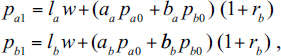
similar to that of the traditional price equations, except of course for the different prices applied to the same good according as it appears as input or as output; for the connected dependence of the level of the uniform effective rate of profit upon the chosen numéraire cf. n. 2 above and passim (for the relation between these undiscounted prices and the discounted ones cf. par. 21, n. 47).
12 It may thus be interesting to note that, had we considered the possibility of storage, system (E) would have needed to be modified by replacing the last two equations in (1.3e) with the following relations:
 |
(1.3e′) |
where Ti is the quantity of commodity i stored (i = a0, b0).
Further, equations (1.1e) in (E) would have to be modified by introducing an inequality sign
| (1.5e′) |
and the following relations would also have to be added
| (1.5e″) |
indicating the price Pi0 low enough to make it convenient to provide the commodity of period t = 1 by the storage of that of period t = 0, at a cost of storage here assumed to consist of a physical wastage αi < 1. Now, the cases will be three, depending on Ti relative to Di1:
1. if Ti = 0, the relation (1.1e′) for commodity i will hold with an equality, and (1.1e″) generally with an inequality;
2. if 0 < Ti < Di1, i.e. the demand for i in t = 1 is satisfied by storage only in part and therefore the needs of i in t = 1 will be partly satisfied by storage and partly by production, both the respective relations in (1.1e′) and (1.1e″) will hold with an equality sign;
3. if finally Ti = Di1, relation (1.1e″) will be satisfied with an equality sign, (1.1e′) being generally satisfied with an inequality.
Conditions (1.1e″) will on the other hand allow determining the two new unknowns Ta and Tb.
13 An example is provided already by equations (1.1e″) in n. 12 which establish a constraint on ‘intertemporal’ prices which has no substantive correspondent for ‘contemporary’ prices. We shall also see (point IV in par. 14, and parr. [7] and [12] in Appendix I) that the principle for which the zero price of one commodity in terms of one scarce commodity, entails a zero price in terms of any other scarce commodity does not appear to apply to intertemporal prices.
14 It should be noted that, contrary to general usage, we need to include in the gross investment, and hence in both ‘gross’ social product and ‘gross’ savings, the replacement of circulating means of production (the only means of production of our model).
15 From the first two equations (1.3e) we obtain Ia0 = A0 − Da0, and Ib0 = B0 − Db0; and since in relations (1.5) we have Sa0 = A0 − Da0; Sb0 = B0 − Db0; we obtain Ia0 = Sa0; Ib0 = Sb0 and, finally, I0 = S0. We have here assumed the relevant relations (1.3e) to be equations. Should the inequality sign apply in any of the two, the corresponding price would be zero and the ‘excess savings’ in that commodity would not affect the value equality, I0 = S0.
16 It may be asked why the income L0W is being excluded from Y0 in equation (1.5) and is included instead in Y1. However, ‘yearly’ production cycles, as distinct from continuous production, force us to distinguish between the period in which the participation of resources to production has occurred (in the present case t = 0) and the period in which the corresponding income must be supposed to accrue, if the equality between the social income and value of the social product is to be maintained. This does not preclude wages being ‘advanced’ in t = 0, but that would be out of the savings of capitalists in t = 0, unlike what we have assumed here in equation (1.5).
17 The relations we are describing are in the nature of accounting identities and would hold whether the economy is in equilibrium or out of it — whether, more generally, they refer to realised savings and investment or, instead, to decisions to save and invest under some a priori specified, hypothetical circumstances. The latter is the case in equations (1.4) and (1.5), where we have applied those relations to the equilibrium quantities of system (E), just as it will be the case when we shall apply them to the partly different hypothetical circumstances of system (F) of the next paragraph, implying equilibrium in some markets and not in others.
18 See the quotation in par. 1, n. 4.
19 We have referred to two own rates of interest for period t = 0. As is well known, when the relative price of the two goods changes from t = 0 to t = 1, arbitrage will impose a lower nominal interest rate for loans in terms of the good, say a, whose relative value rises from t = 0 to t = 1, in order to compensate the advantage its lender would other-wise have relative to lenders of b, and so as to realise what is in effect a uniform rate of interest. This rate takes then a numérical expression dependent on the numéraire, not unlike what happens for commodity prices (cf. n. 2 and Appendix I, par [9]).
20 Cf. n. 8, 15. The nature of these two constructs can perhaps be more easily grasped when we realise that they follow the simple logical procedure which underlies, in an elementary textbook, the representation of, say, the demand for labour, when the quantity demanded LD is directly derived from the marginal product of the labour employed with the given supply λ of land, the only other productive factor. At any point along that demand schedule, the following equations will therefore hold:
![]()
The wage w is the independent variable, leaving four unknowns in the four equations, i.e. the corn output Q, the rent rate ρ and the quantities demanded and supplied LD and LS of labour, where for simplicity we have supposed the factor supplies LS and λ to be rigid. At any relevant level of w, equilibrium will hold in the remaining two markets: for corn, where Q is equal to the corn expenditure (LDw + λρ) from the owners of the two factors, and for land, where the supply λ is fully employed. The two schedules LD(w) and LS = constant resulting as w varies, will therefore be ‘general equilibrium schedules’ in the sense market, i.e. when either LD = LS, or LD < LS with W = 0, or LD > LS and the wage is at its maximum for which ρ = 0. We may note for future reference how that disequilibrium in a single market — that of labour — is here compatible with the sum of budget equations (Walras’s law) because the labour income in the economy is taken to be LDw, i.e. that corresponding to the quantity LD of labour demanded, and not to the endowment LS: cf. par. 9 in this text for the similar problem in the savings-investment market.
We may also note how the schedules may clarify the economic rationale of the necessary existence of an equilibrium, once excess supplies of factors are admitted for a zero price of their services. Not only an excess supply LS > LD permits an equilibrium for w = 0, but also an excess demand LS > LD does so for w at its maximum, since that situation is, in fact, just the same case with land in the place of labour: i.e. excess supply of land with zero rent, when land used can be scaled down to employ no more than the labour supply so any relative position of the schedules entails equilibria. Once excess supply and zero prices are admitted, the existence of solutions can be seen as a rather clear implication of the aggregate of budget equations (and, of course, of the continuity of the functions). Uniqueness, stability and more generally plausibility of the “equilibria” are what the neoclassical demand and supply rested on and the principle of substitution was for.
21 See par. 9 (and the preceding footnote), for the ‘adjustment in expenditures’ which allows the disequilibrium to be confined to the single market of savings and investment.
22 The changes in methods of production which we might expect to occur along the schedules as rb varies will be introduced in Section 1.5. It should however be noted that the schedules determined by (F) would already allow for the ‘substitutability’ between factors arising from consumer choice in t = 1.
23 The fact that the single market for I and S involves in effect the two markets, for a0 and b0, is irrelevant here.
24 The question is essentially the same as the one concerning the adjustment in the power to purchase ‘corn’ in the simple example of general equilibrium demand for labour of par. 6, n. 20 above. We implied that adjustment when we attributed an income only to the workers employed LD. In the present model, let us indicate by Db1′, Da1′, the consumption demands in t = 1 resulting from the equations of consumer equilibrium on the usual hypothesis that they dispose of the income resulting at the given prices from all the resources they own. Summing the budget equations through consumers and the two ‘years’, we get, after some simple transformations,
| (1.8a) |
Clearly the L.H.S. of equation (8a) gives both the social income Y1′, and the value of the purchases the individuals would carry out at t = 1, under the stated assumptions of complete sales of A0S, B0S, besides L. Then using relation (1.5) of par. 4, we have
| (1.8b) |
On the other hand, the value Q1 of the gross social product for t = 1, as it results from the system (F) by substituting for prices in accordance with equations (1.1f), is given by
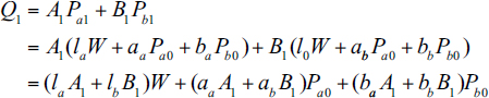
and using equation (1.4f),
| (1.8c) |
Thus the purchasing power (S+LW) in equation (1.8b) would face commodities of the value (I+LW) in equation (1.8c), and if we had used Db1′, Da1′, in the system (F), the system would have been inconsistent. The ‘adjustment’ of purchases mentioned in the text can, on the other hand, be represented by the following equations, in which we indicate by Di1, as distinct from Di1′, the ‘adjusted’ purchases in t = 1 appearing in our system (F):

It follows that the ‘adjusted’ aggregate expenditure and income Y1 in t = 1 is now given by

and consistency has been brought back into the system (F). We may note that, by definition, consumption purchases for t = 0 remain unchanged, i.e. Db0 = Db0′, Da0 = Da0′, and so does therefore S, the amount of the decisions to save in t = 0.
25 Apparently less plausible is the behaviour assumed in the opposite case of I > S, where the purchases for t = 1 would have to exceed what is possible with the purchasing power obtained from the full sale of the A0S and B0S endowments. However, the extra purchasing power implied in our adjustment of expenditures may be taken to express the tendential relative rise of purchasing power available in t = 1 because of the excess demand in t = 0 and a resulting tendential rise in the prices of commodities a0 and b0 (in terms of which savings are effected) relative to those of a1 and b1.
26 Cf.: ‘Unfortunately, necessary conditions are unlikely to be available’ (Arrow, Hahn, 1971: 242).
27 See e.g. Marshall (1949: 109–110, 391n, 665); Walras (1954: 112–113); Wicksell (1934: 56–61).
28 See e.g. Kirman (1989).
29 Thus Hicks could conclude in 1939 about the stability of equilibrium in exchange, and with reference to income effects:
It cannot indeed be proved a priori that a system of multiple exchange will be necessarily stable. But the conditions of stability are quite easy conditions, so that it is quite reasonable to assume that they will be satisfied in almost any system with which we are likely to be concerned.
(Hicks, 1939: 72)
and he even thought that such a conclusion could be strengthened when introducing production (1939: 104).
30 See e.g. the distinction between ‘intertemporal’ and ‘contemporary’ relative prices in par. 3. (For its implications, cf. point V in par. 14 and par. 8 in Appendix I).
31 Essentially, the resort to a sub-case has occurred once, namely for the monotonic rising change of Pa0 as rb rises (cf. point II in par. 14 below).
32 They are not of course perfect substitutes in production.
33 See above, n. 2.
34 Thus in Value and Capital, 1939, where the new notions of equilibrium and the associated ‘dating’ of equilibrium variables were used for perhaps the first time in influential Anglo-American work, Hicks felt forced to assume that transactions carried out at non-equilibrium prices would have very little effect on the amounts transacted, so that equilibrium prices could be realised on his ‘Mondays’ (1939: 127–128: the stability of those equilibria was evidently taken for granted). However, both in that book and in much subsequent work in pure theory, it is not mentioned that the question in the preceding literature was that of a compensation of deviations through repetition, and not that of the price actually hitting its equilibrium level. Thus Bliss (1975) refers to the ‘Herculean programme’ of constructing ‘the complete theory of the behaviour of the economy out-of-equilibrium’ necessary, in his view, in order to validate equilibrium ‘as something that would be expected to be realised’ apparently overlooking that repetition of transactions on unchanged data and not the truly Herculean ‘complete theory etc.’ had been the question — so long as one could rely on the traditional notion of equilibrium. We get however closer to the basic difficulty, when Bliss continues
Furthermore, even if equilibrium were to be stable there might not be enough time within the space of a “week” for the prices to adjust to an equilibrium
(Bliss, 1975: 28)
where Bliss sees the importance for the significance of the equilibrium of a sufficient lapse of time under approximately unchanged data. But, then, why not an equilibrium like the traditional one which would last more than a week, without falling in the limited relevance of the “steady state”? Here again (cf. n. 5 above) Bliss does not seem to ask himself the question, clearly relevant for the theory of capital to which he devotes his book (we shall indeed see in the Appendix II, par. viii, the very particular way in which he reconstructs the traditional equilibrium of Wicksell).
35 Walras introduced re-contracting only in the 4th edition of the Elements (1900). In the previous editions, the word tâtonnement had covered only the process of repetition of actual transactions, which in his view (confirmed up to the posthumous 4th ‘definitive’ edition of 1926):
is perpetually tending towards equilibrium without ever actually attaining it (…) like a lake agitated by the wind where the water is incessantly seeking its level without ever reaching it.
(Walras, 1954: 380)
Re-contracting with ‘bons’ (tickets) was introduced in the 4th edition of 1900 and exclusively in order to avoid considering the changes occurring in the capital stocks during the process of gravitation around the equilibrium (1954: 242 and Jaffè’s collation note [h] pp. 582–583; Garegnani, 1960). Thus, it seems, recontracting was adopted in order to rigorously analyse a real repetition of transaction (in which, he thus implied, changes in the capital stocks over the relevant period would not make appreciable difference) and not in order to have a notional repetition of transactions when a real one was prevented even in principle by the dating of the equilibria.
36 The level rb > rbmin entails Pb0 > 0 and hence, by assumption (iii) par. [5], Appendix I, Pa0 > 0.
37 Thus, should the schedules be representable as in Figure 1.2 below, intersection D would not indicate an equilibrium because, of the two successive (F) positions, (F′) and (F″), that we meet in sequence at rb as LD falls from the full employment level of I+ and S+, point D corresponds to (F′) on the I schedule, but to (F″) on the S schedule. Intersections E1 and E2 however are equilibria since each corresponds to the same (F) position on both schedules.
38 Except for the fluke case of Sa = Ia, and therefore, Sb = Ib exactly achieved for rb = −1, which would of course be compatible with both S > I and I > S in the proximity of rbmin
39 It would be correct to say that the cause of the possible rise of one own rate, call it ra, as the other falls because of excess savings, is quite different from the excess savings, which cause the other to fall and would generally make for a fall of both rates. A fall of all consumption goods prices for t = 0, relative to those for t = 1 is in fact what we would expect from excess savings, i.e. excess supply of consumption goods in general in t = 0, and excess demand for them in general in t = 1. A rise of ra as we move along the schedules because of excess savings can only result from a strong dislocation of contemporary relative prices for which the relative price of a to b were to rise for more between t = 0 and t = 1 than it did at higher levels of rb (cf. Appendix I par. [9]).
A seeming puzzle connected with opposite movement of the own rates should perhaps be sorted out at this point. Should ra rise in the proximity of an equilibrium as rb falls because of excess savings, would not a representation of the same (F) position with ra in place of rb on the vertical axis (see Figure A) lead to opposite conclusions about the stability of the equilibrium? The answer is of course negative since the adjusted spontaneous competitive change consequent to excess savings would, with an apparent paradox, be a rise and not a fall of the interest rate — owing to the change in the relative-prices factor of equation (1.6d in loc. cit. Appendix I). Figure A below illustrates the ‘upside-down’ representation of an equilibrium E and of the neighbouring positions (F′) and (F″) when ra is put on the vertical axis.
40 40 As I remarked in (1991: 359) arguments about stability conducted like the one here, confined essentially to signs of changes, while finding ready confirmation in competitive behaviour, ‘are by their nature quite general [and] render … possible equally general conclusions’.

Figure A Should the own commodity rates ra and rb change in opposite direction in moving from a position (F′) of the economy with S′ > I′ to a position (F″) with only rb falling as indicated by the arrow in diagram (i) — then the spontaneous competitive movement in diagram (ii), with ra on the vertical axis, would be upwards
41 No tendency would be there to the ‘fluke’ equilibrium mentioned in n. 38 when Sa = Ia, Sb = Ib at rbmin but S < I as rb → rbmin.
42 Marginal products, whether of the discontinuous or the continuous variety, require that the available techniques be susceptible of being ordered so that they can be made to differ by the quantity of only one factor at a time. That, it seems, cannot generally be done when the factors are more than two: weighted averages of the different methods available which could give the above result will not make general economic sense, since it would be an exception when the methods entering such averages could coexist.
43 A sufficient unanimity concerning the technique to be adopted has evidently to be assumed in order to let the corresponding prices emerge from the re-contracting. That unanimity has then to be replaced by a similar one concerning a second technique which had been found to be cheaper at those earlier prices, and so on and so forth. The way out of this conundrum is of course the further fiction of the auctioneer.
44 For the question in its traditional context, cf. Sraffa (1960, Chapter xii) and the subsequent literature referred to in Kurz and Salvadori (1995: 151).
45 Comparisons regard in fact methods of production of each commodity rather than techniques: and changes in technique, in particular those leading to the cheapest technique i, are best envisaged as resulting from changes of methods for one commodity at a time. However, referring to techniques, as above, rather than to methods, has no drawback here when one remembers that there will then be no one-to-one correspondence between method and technique, the same method appearing in several techniques differing from each other by the method of the remaining commodity.
46 Cf. Garegnani (1978–1979: I).
47 To make rb appear explicitly in equation (10b) we should turn to the undiscounted prices, here indicated by the small letter p. (cf. n. 11 above). By itself, this change in the equations does not, of course, entail any change in the assumptions of the model (in particular in the assumption of complete future markets or of an ‘initial’ contracting period): it only requires that each price be notionally referred to the date of delivery of the good by taking as numéraire for it. the good b of the same date. Then the wage W and the undiscounted prices of a1 and b1, are numerically equal to the discounted ones because already expressed in terms of b of t = 1
![]()
As for the undiscounted prices of a0 and b0, using equation (1.6f) we have:
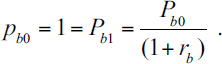
and since Pb0 = 1 + rb, we also have
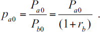
The two relations (1.1f) can then be written as follows:
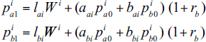 |
(1.3fi′) |
and the first equation of each couple (1.8fi) is
| (1.9fi′) |
Expressing now the undiscounted capital expenses as
 |
(1.10′) |
By transformations analogous to those operated in passing from equations (1.10) to (1.10b) in the text, we obtain
 |
(1.10b′) |
where the change in the pai0/paj0 can now be seen to depend on the ratio (1+rb)/W.
48 For an example cf. the quotation in par. 1, n. 4.
49 Equation (1.5b) holds before the adjustments of purchasing power mentioned in par. 9.
50 Thus it seems incorrect to hold, with evident reference to reverse capital deepening and the reswitching of techniques, that
it is only because we want to have some kind of geometric average, called the rate of interest, that we get some of these paradoxes.
(Arrow, 1989: p. 155)
The paradoxes are present, whether we refer to the intertemporal prices which, as Arrow states there, are ‘what we are really interested in’, or to the single rate of interest in the case of the traditional equilibrium. Only the language for describing them changes (cf. n. 39 above).
51 It perhaps ironical that Keynes should have been incorrect when he wrote: ‘If savings consisted not merely in abstaining from present consumption but in placing simultaneously a specific order for future consumption, the effect might indeed be different. For in that case the resources released from preparing for present consumption could be turned over to preparing for the future consumption’ (Keynes, 1936: 210–211). In fact the order for future consumption could remain unfulfilled if the reaction of the interest rates failed to incentivate entrepreneurs to ‘deepen’ capital in the economy. However, the ‘might’ we have italicised indicates, perhaps, Keynes’ doubt that his ‘struggle of escape from habitual modes of thought’ (1936: p. viii) could have gone further.
52 Cf. e.g. ‘Certainly … we should not be much interested in an equilibrium with a zero real wage’ (Arrow and Hahn, 1971: 354–355).
53 It may seem paradoxical that it should be excess investment that accompanies here labour unemployment. However in the model, excess investment is excess demand for the given stocks of a0 and b0, with whose owners labour competes in sharing the product available in t = 1 (see equation (1.1a) in Appendix I, par. [2]): zero wages due to deficient investment need at least three periods in order to emerge.
54 To a (1970: 422) statement of mine to the effect that the neoclassical explanation of distribution rests essentially on the premise that a fall of the rate of interest must increase the ratio of ‘capital’ to labour in the economy, Chistopher Bliss reacted by writing ‘If by explanation of distribution the author means equilibrium theory (say of the intertemporal economy) then he has dreamed up this condition’ (1975, 117). What we just saw in the text might now convince Bliss that dreams can indeed be prescient — of course if one regards as relevant for intertemporal “equilibrium theory” the possibility of zero wages or negative interest rates in its equilibria.
55 Walras (1954: 274 ff). Of course it is difficult to define ‘perpetual future income’ in an intertemporal equilibrium, rather than in the traditional long-period equilibrium of Walras’s system (par. 1, n. 2). However, the essential nature of savings in neoclassical theory as demand for a homogeneous commodity ‘future income’ remains the same.
56 Walras’s point incidentally explains why competitive arbitrage tends to achieve a uniform rate of return over any (however short) period by acting on the demand price of the capital good, and lowering it below its supply price when the rate of return on the latter is below that of other capital goods. But the prices of capital goods, like those of any product, tend to equality with the respective supply prices in the Marshallian long period, and Walras’s single price will turn out to obtain on the supply prices of the capital goods as Walras and the present discussion imply.
57 The need for that ‘quantity’ is in fact strictly connected with neoclassical theory. The perfect substitutability among capital goods for wealth holders does not impose the notion of an independently measurable quantity of capital in the classical theories, where the rate of interest (profits) is not explained in terms of individual demand and supply decisions about ‘factors of production’ and is instead obtained, essentially, as a difference between product and wages determined separately from prices.
58 See n. 2 above.
59 Cf. n. 8 above.
Notes for Appendix I
1 Paragraphs in this Appendix are numbered in square brackets to distinguish them from those of the main text.
2 Should b0 be storable, its intertemporal price Pb0/Pb1 could not fall below unity, or below (1 − αb) when storage for a year implies costs ab (cf. equations (1.1e″), n. 12 in the text), and rb could not accordingly fall below zero, or (−αb) respectively.
3 E.g. we cannot exclude that at some relative price Pa0/Pb0 a consumer be indifferent between the two goods within certain limiting proportions of them: all quantities staying within those limits would then be demanded at the corresponding single price. (This question, which concerns multiplicity of quantities demanded at given prices should of course not be confused with ‘income effects’, which may cause multiplicity of prices for the same quantities demanded: par. [5]).
4 In fact the rise of Pa0 together with rb (par. [5]) will lower the economically relevant upper limit of both rb and Pa0 below those of relations (1.6c) and (1.1b).
5 5 The device would consist of somewhat counterintuitively dissociating the total quantities A0U, B0U of the two commodities ‘used’ for consumption and investment, from the respective quantities ‘demanded’ A0D, B0D appearing in equation (1.7f). Provided the price of the commodity in question is zero, we could then let the quantity ‘demanded’ A0D or B0D exceed the respective one used A0D or B0D, by allowing for inequalities in the corresponding relations [1.3f], where the R.H.S. expresses B0U, A0U, respectively, and in that way satisfy equation (1.7f).
6 A lowering of Pa0/Pb0 would tend to lower the relative price Pa1/Pb1 of the good requiring more of a for its production (provided the relative labour intensities in the production of a and b do not cause the variation of the wage to more than compensate that effect) and with the proportion consumed of that good increasing, the proportion Ia /Ib would also increase.
7 It might on the other hand seem that having in common W = 0, such a continuum of solutions of (F) would have in common also the contemporary relative price π = Pa0/Pb0 and the rest of the price system with it, so that a single level of rb = rb+ = rbmax, and the corresponding single set of prices, would hold over the whole continuum for W = 0.
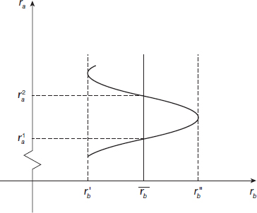
Figure B As the own rate rb″ falls from rb″ to rb′ a rise or constancy of the own interest rate ra, as depicted in the figure, is incompatible with the monotonic increasing relation between Pa0/Pb1 and Pb0/Pb1 of Assumption (iii) in par. 4
However zero total wages LDW mean that Q1, the value of the product in t = 1 (par. 9, n. 24 .in the text) along the continuum, is given by
Q1 = S = Da1 Pa1 + Db1 Pb1.
Now, if prices were not to change along that continuum, the ratio Da1/Db1 would be constant, and so would then be the ratio Ia/Ib, though the absolute levels of Da1, Db1 and therefore Ia, Ib would be falling as LD falls (see the adjustment to the level of I of the purchasing power in t = 1, described in the main text: par. 9, n. 24). Since Da0 and Dbo would instead be constant also in their absolute amounts, it would follow that, A0D/B0D, a weighted average of Da0/Db0 and Ia/Ib (see the first two equations (1.3f)), would generally be changing with LD. This imposes a change in the contemporary price π (and hence the other prices) in order to continue to satisfy equation (1.7f).
8 It may be useful to note that rb0, although no greater than rb+, must be larger than rbmin. Since Pb0 = 0 would entail Pa0 = 0 (par. [11]), equation (1.1c), valid for W = 0, is only compatible with Pb0 > 0, and therefore with rb0 > rbmin.
9 Formally we replace equation (1.7f) with an equation Pa0/Pb0 = constant, and treat A0D/B0D as an unknown.
10 Suppose that not to be so and thus ra to fall as rb rises in a sub-interval rb′ < rb < rb″ included in the overall interval rbmin < rb < rb0 (see Figure B). At least two distinct levels, ra1 and ra2 would have to correspond to any given level ![]() b in that sub-interval, since ra must have initially risen from ramin = −1, together with rb, as Pa0/Pb1 rose monotonically from zero together with Pb0/Pb1 (Assumption (iii); and par. 11 below). However, that same monotonic relation between Pa0 and Pb0 entails that the two levels Pa01 and Pa02 corresponding to ra1 and ra2 respectively, would be equal because they correspond to the single value
b in that sub-interval, since ra must have initially risen from ramin = −1, together with rb, as Pa0/Pb1 rose monotonically from zero together with Pb0/Pb1 (Assumption (iii); and par. 11 below). However, that same monotonic relation between Pa0 and Pb0 entails that the two levels Pa01 and Pa02 corresponding to ra1 and ra2 respectively, would be equal because they correspond to the single value ![]() b0 =
b0 = ![]() b + 1. But then Pa01/Pb0 = Pa02/Pb0 would have in common the same unique series of prices (par. 2), and therefore ra1 = ra2, contrary to our premiss. The same monotonicity of the relation between Pa0/Pb1 entails that ra cannot remain constant as rb changes: for that to happen two levels of rb and therefore of Pb0, i.e. Pb02, Pb01, should correspond to the level Pa0 holding for the given ra.
b + 1. But then Pa01/Pb0 = Pa02/Pb0 would have in common the same unique series of prices (par. 2), and therefore ra1 = ra2, contrary to our premiss. The same monotonicity of the relation between Pa0/Pb1 entails that ra cannot remain constant as rb changes: for that to happen two levels of rb and therefore of Pb0, i.e. Pb02, Pb01, should correspond to the level Pa0 holding for the given ra.
11 This can only happen for a part of the relevant interval of rb, since ra has to rise from −1 as rb does (see the preceding endnote).
12 A position which we find exemplified in Morishima (1964: 87) is to assume, at a zero wage, both a zero supply and the continuity of the supply schedule for labour. It might seem possible to reconcile this position with the question of ‘survival’ discussed in the text, by assuming a nearly horizontal segment joining the origin of the axes with a comparatively high level of labour supply for a wage close to zero (a strictly horizontal segment would instead be the graphic representation of the kind of continuity we are assuming). However, it is not easy to see why a worker who has been increasing his labour supply to try to survive, should abandon that purpose by progressively decreasing his supply when the wage is still positive: a discontinuity of supply would rather seem natural when the worker gives up hope of survival. Even more arbitrary seem to be other assumptions ensuring continuity, such as e.g. that of each individual being endowed with some quantity of each resource (Debreu, 1959: 19) i.e. of a quantity of some other resource whose price is bound to rise when that of the resource considered tends to zero, thus avoiding dependence on the latter for survival.
13 We are here referring to general-equilibrium-demand and supply schedules for labour, obtained from (E) by treating W as an independent variable, and using the third of relations (1.3e) to define the new unknown labour demanded LD, with an adjustment in aggregate expenditure analogous to that we saw in par. 9, n. 24 in the text.
14 The discontinuity would result from savings suddenly disappearing, at rb = −1 with a0 and b0 being used instead entirely for consumption in t = 0 at the ‘contemporary’ price π = Pa0/Pb0, ensuring relative consumption demands Da0/Db0 compatible with (1.7f). It is also possible to envisage that, through consumption loans, wage income (reaching its maximum, as rb and ra fall towards their minimum) be spent in advance by increasing consumptions Da0, Db0 of both goods as their intertemporal prices relevant here fall towards zero: this could engender negative gross savings in the lower range of the S curve, and savings could become zero at some level rb > rbmin.
15 This arbitrage condition like any arbitrage conditions entailed by indirect exchanges is implied when reducing the number of prices from that of all combinations of the n commodities taken two by two, down to (n−1). Thus e.g. Pb0/Pb1 = 0 entails that in Pb0/Pb1 = (Pb0/Pa1)(Pa1/Pb1) = 0, with Pa1/Pb1 ≠ 0, we should have Pb0/Pa1 = 0. This, so to speak, ‘collective’ zero intertemporal price of commodities dated t = 0, in terms of commodities dated t = 1 confirms on the other hand that capital goods a0 and b0 are perfect substitutes for the savers acquiring them (parr. 25–26 in the text) so that the zero intertemporal price of one entails a zero price of the other. The reader may however wonder how it will be possible to discriminate in practice between, on the one hand. producers of b1 or a1, who would get b0 and a0 for free, and owners of a0 and b0 who should instead give some of their commodity in order to get the other.
16 Cf. par. 3. The only difference is that for rb = −1, i.e. Pb0 = 0, equation (1.2f) of par. 4 gives the intertemporal price Pa0 = 0.
17 Given the possible multiplicity of solutions of (F) in the interval rb0 ≤ rb≤ rbmax, the determination of the (F) positions for W = 0 is most easily envisaged by the device of letting LD (which is uniquely related to those positions) to take the role of independent variable when W = 0, so as to obtain the corresponding rb and with it all the other unknowns of the (F) system for that level of LD. In particular this will allow tracing the multiple (F) positions which may correspond to the same level of rb for W = 0.
18 Assumption (iii) of par. [5], on the joint rise of Pa0/Pb1 and Pb0/Pb1 so long as W > 0, excludes that among the multiple solutions for rb0≤ rb ≤ rbmax, there may be any with a positive W, apart from those on the ‘main branch’ of the function relating π = Pa0/Pb0 and rb.
19 Contrary to what one might think at first, the income from which those savings come, is likely to change little as LD changes since, with W = 0, only the owners of the initial stocks A0S and B0S will have an income (cf. n. 7) — the adjustment in the expenditure for t = 1 described in par. 9 of the text then taking care of the changes in the physical social product for that period as LD changes.
Notes for Appendix II
1 See par. (v) about the capital endowments of Hahn’s ‘Special’ case. Cf. Garegnani (1990b: 113–115) for an answer to Hahn’s (1982) first claim. We may also note that in (1975: 361) Hahn finds ‘incomprehensible’ the ‘neo-Ricardian’ idea that ‘distribution precedes value’. However, it was in (1951, xxx–xlviii) that Sraffa had advanced his interpretation of Ricardo and the old classical economists in terms of a wage determined by historical and institutional circumstances (‘subsistence’), with the non-wage distributive variables accordingly resulting as a residue or surplus. This interpretation, where in an evident sense distribution (the determination of the real wage) precedes values, had indeed been expounded and variously discussed before, with, and after, Sraffa (1960), also with respect to its distinction from the alternative theory advanced by Joan Robinson in 1956 and her other works.
2 Cf. e.g. Hutchison (2000); Blaug (1999).
3 Cf. equations (22) in Hahn (1982: 364) corresponding to our equations (1.1e) of par. 3 in the chapter; his equation (17), p. 363, for our (1.2e); then (25), p. 365, for the first three of our relations (1.3e) and, finally, equations (23), p. 364, for the remaining two of relations (1e).
4 Cf. equations [25], in Hahn (1982: 363). Hahn does not, on the other hand, assume ‘activities’ of free disposal and justifying those equality signs.
5 Cf. n. 7 below. For the distinction between demand and supply prices of capital goods, cf. e.g. Walras’s distinction between the ‘prix de vente’ and the ‘prix de revient’ of such goods, which Jaffé translates in his edition as ‘selling prices’ and ‘costs of production’ respectively (Walras, 1954: 271 ff.).
6 Of course obsolete capital goods are not supposed to be produced but neither can they be present in the physically specified endowment of an economy like that of Walras (1954) and Hahn (1982) where only the dominant methods of production appear. I owe to Professor Fabio Petri having attracted my attention to the point.
7 See Garegnani (1990a: 11–22); on the point in Walras’s own texts, cf. also by the same author (1958) and (1960), Part II, Chs. II and III. In Appendix G of the (1960) book, I also noted how Pareto, who in the Cours (1896–97) had already been ambiguous as to whether all capital goods were being produced, finally abandoned in his Manuel (1906) any attempt to formalise the theory of capitalisation. (The overdeterminacy of Walras’s system becomes evident if we refer to the extreme case of absolute redundancy in the endowment of one capital good, with its rate of return on the supply price being accordingly zero or negative, and obviously less than that of any scarce capital goods).
8 Cf. Hahn (1982: 365–366) where it is suggested that B0 be treated as an unknown, while keeping A0 as a given.
9 One may be curious about the reason why in Hahn’s model letting the proportion between the two capital goods in the endowment be an unknown will instead ensure constancy of prices. That has to do with the peculiarity of a model which admits of one production cycle only. By starting from a sufficiently high stock A0S relative to stock B0S (see par. 6 in the text) and then lowering it sufficiently, we may generally continuously change Pa0/Pb0 so that it rises from zero to infinity: i.e. from a0 being a free good to b0 being such. There must then be at least one proportion A0/B0 of the two stocks for which the curve described by the relative price Pa0/Pb0, with A0/B0 in the abscissae intersects the analogous curve described by the production prices Pa1/Pb1 of equations (1.1e) of par. 3 in the text, thus giving ra = rb. However, as soon as a second yearly cycle of production is allowed for, and price equations must be satisfied also for Pa2 and Pb2, the same relative prices could be maintained for a third year only if the economy happened to be stationary (or the technical conditions of production allowed for a labour theory of value).
10 Cf. e.g. Hicks (1939: 118) and Garegnani (1960, Appendix E). This of course does not detract from the fact that a constancy of relative prices will generally imply also an adjusted physical composition of the capital stock.
11 See the references in n. 7, and Garegnani (1976: 38–39). The results are reported, e.g. in Harcourt (1972: 170, 171), J.Robinson (1970: 338), Dobb (1973: 205 n).
12 Cf. par. (iv) and n. 8.
13 As just mentioned Hahn (1982) does not recall that this ‘specialisation’ was traditionally achieved by treating capital as a homogeneous substance so that the proportions between capital stocks were in fact unknowns, and not ‘specialised data’ which ‘history’ had happened to throw up (par. [xi]).
14 On this failure to distinguish the basic form (b) of uniformity of returns on capital characterising a normal position of the economic system from Adam Smith down to recent decades, from the uniformity (a) between own rates due to price constancy and, besides, from the short period uniformity imposed by arbitrage (and to be presently considered in this Appendix), see e.g. Christopher Bliss’s New Palgrave article dedicated to the ‘Equality of Profit Rates’. Under what he calls ‘the rate of profit’ Bliss does not appear to distinguish between the above short-period uniformity on the demand prices of the capital goods and the uniformity on the supply prices, the one traditionally indicated as the ‘uniform rate of profit’. The uniform ‘rate of profit’ is instead counterposed to the divergence of own commodity rates of interest which, as in Hahn, accordingly appears to be taken as one with the divergence of effective returns on the supply prices of the capital goods which the critics had indicated as a shortcoming of contemporary theory.
15 Cf. n. 2.
16 Such an attentive reading of the relevant part of Hicks’s Value and Capital shows, I believe, that the difficulty Hicks was trying to overcome was not that of the change of equilibrium prices over time: but rather that of the ‘quantity of capital’ — as, on the other hand, he indicated by the very title of his book (on the point, cf. Garegnani, 1976: 30–36; Milgate, 1979: 6–9).
17 Cf. n. 8 in the text and n. 10 here.
18 Possibilities of substitution would still enter the system as the physical composition of the stock can change by means of capital replacement: but then, as argued in the main text, we are back to ‘capital’ as a single quantity and its problems through the relation between gross investment and the interest rate.
References
Arrow, K.J. (1989). ‘Joan Robinson and Modern Economic Theory: an Interview’, in G.R. Feiwel (ed.), Joan Robinson and Modern Economic Theory, London: Macmillan.
Arrow, K.J. and Hahn, F.H. (1971). General Competitive Analysis, San Francisco: Holden-Day: Edinburgh: Oliver & Boyd.
Blaug, M. (1999). ‘The Formalist Revolution or What Happened to Orthodox Economics after World War II?’, in R.E. Backhouse and J. Creedy (eds), From Classical Economics to the Theory of the Firm. Essays in Honour of D.P.O’Brien, Cheltenham: Edward Elgar.
Bliss, C.J. (1975). Capital Theory and the Distribution of Income, Amsterdam: North-Holland.
Bliss, C.J. (1987). ‘Equal Rates and Profits’, in J. Eatwell, M. Milgate and P. Newman (eds), New Palgrave Dictionary of Economics, London: Macmillan.
Böhm-Bawerk, E.v. (1891). The Positive Theory of Capital, London: Macmillan. Translation of the 1st edn of Böhm-Bawerk (1889).
Currie, M. and Steedman, I. (1990). Wrestling with Time. Problems in Economic Theory, Manchester: Manchester University Press.
Debreu, G. (1959). The Theory of Value, New York: John Wiley.
Dobb, M. (1973). Theories of Value and Distribution Since Adam Smith: Ideology and Economic Theory, Cambridge: Cambridge University Press.
Eatwell, J.L. (1987). ‘Walras’s Theory of Capital’, in J. Eatwell, M. Milgate and P. Newman (eds), New Palgrave Dictionary of Economics, Vol. 4, London: Macmillan.
Garegnani P. (1958). A Problem in the Theory of Distribution from Ricardo to Wicksell, Cambridge University, Ph.D. Thesis.
Garegnani, P. (1960). Il capitale nelle teorie della distribuzione, Milano: Giuffrè.
Garegnani, P. (1970). ‘Heterogeneous Capital, the Production Function and the Theory of Distribution’, Review of Economic Studies, 37, pp. 407–436.
Garegnani, P. (1976). ‘On a Change in the Notion of Equilibrium in Recent Work on Value and Distribution’, in M. Brown, K. Sato and P. Zarembka (eds), Essays on Modern Capital Theory, Amsterdam: North Holland.
Garegnani, P. ([1978] 1979). ‘Notes on Consumption, Investment and Effective Demand’, Part I and Part II, in Cambridge Journal of Economics, 2, pp. 335–353, and 3, pp. 63–82.
Garegnani, P. (1990a). ‘Quantity of Capital’, in J. Eatwell, M. Milgate and P. Newman (eds), Capital Theory, London: Macmillan.
Garegnani, P. (1990b). ‘Sraffa: Classical versus Marginalist Analysis’, in K. Bharadwaj and B. Schefold (eds), Essays on Sraffa, London: Routledge.
Garegnani, P. (1991). ‘On Some Supposed Obstacles to the Tendency of Market Prices Towards Natural Prices’, Political Economy, 6, pp. 329–359.
Garegnani, P. (2000). ‘Savings, Investment and Capital in a System of General Inter temporal Equilibrium’, in H.D. Kurz (ed.), Critical Essays on Piero Sraffa’s Legacy in Economics, Cambridge: Cambridge University Press.
Garegnani, P. (2003). ‘Savings, Investment and Capital in a System of General Inter temporal Equilib rium’, in F. Petri and F. Hahn (eds), General Equilibrium: Problems and Prospects, London and New York: Routledge, pp. 117–172.
Hahn, F.H. (1975). ‘Revival of Political Economy: The Wrong Issues and the Wrong Argument’, The Economic Record, 51, pp. 360–364.
Hahn, F.H. (1982). ‘The Neo-Ricardians’, Cambridge Journal of Economics, 6, pp. 353–374.
Harcourt, G.C. (1972). Some Cambridge Controversies in the Theory of Capital,Cambridge: Cambridge University Press.
Hicks, J.R. (1932). The Theory of Wages, London: Macmillan.
Hicks, J.R. (1939). Value and Capital, 2nd edn, London: Oxford University Press.
Hutchison, T. (2000). On the Methodology of Economics and the Formalist Revolution, Cheltenham: Edward Elgar.
Jevons, W.S. ([1871] 1957). The Theory of Political Economy, New York: Kelley.
Keynes, J.M. (1936). The General Theory of Employment, Interest and Money, London: Macmillan.
Kirman, A. (1989). ‘The Intrinsic Limits of Modern Economic Theory: The Emperor Has No Clothes’, The Economic Journal, 99, Supplement, pp. 126–139.
Kurz, H.D. and Salvadori, N. (1995). Theory of Production: A Long Period Analysis, Cambridge: Cambridge University Press.
Marshall, A. ([1920] 1949). Principles of Economics, London: Macmillan.
Morishima, M. (1964) Equilibrium, Stability and Growth, Oxford: Clarendon.
Pareto, V. (1896–7). Cours d’Economie Politique, 2 vols. Lausanne: Librarie de l’Université.
Pigou, A.C. (1932). The Economics of Welfare, 4th edn, London: Macmillan.
Robinson, J.V. (1970). Review of C.E. Ferguson, ‘The Neoclassical Theory of Production and Distribution’, Economic Journal, 80, pp. 336–339.
Samuelson, P.A. (1962). ‘Parable and Realism in Capital Theory: The Surrogate Production Function’, Review of Economic Studies, 29, pp. 193–206.
Sraffa, P. (1960). Production of Commodities by Means of Commodities. Prelude to a Critique of Economic Theory, Cambridge: Cambridge University Press.
Walras, L. (1926). Elements d’Economie Politique Pure, 4th and definitive edn, Paris: F. Richon.
Walras, L. (1954). Elements of Pure Economics, London: Allen & Unwin. English translation of the 4th definitive edition of Walras (1874) by W. Jaffé.
Wicksell, K. (1893). Über Wert, Kapital und Rente nach den neueren nationalökonomischen Theorien, Jena: Gustave Fischer. English translation as Wicksell (1954).
Wicksell, K. ([1901] 1934). Lectures on Political Economy, Vol. 1, London: Routledge & Kegan.
COMMENT ON GAREGNANI*
Bertram Schefold
It is generally agreed that the paradoxes of the theory of capital, uncovered in the so-called debate on reswitching in the 1960s, undermine the validity of neoclassical theory, to the extent that it is based on productive functions and steady state comparisons. It has remained controversial whether general (inter temporal) equilibrium theory is also affected as I have argued in three earlier papers. They demonstrate that general equilibrium paths involving changes of techniques with reswitching are associated with counterintuitive parallel movements of factor prices and factor quantities; they generate, moreover, at least local instabilities. The aim of the present paper [complete version: Schefold 2008] is to explain the method used by P. Garegnani to prove that the paradoxes of capital imply difficulties for general equilibrium theory, and to evaluate advantages and shortcomings of his approach, but we first give our intuitive reason why such instabilities exist.
The choice of technique among methods (input vectors) a0, a1, a2 with labour l0, l1, l2, is introduced by assuming that there are two alternative processes in the first industry of a model with two sectors, producing two commodities in single production, so that we have two techniques

We analyse the systems first as in Sraffa (1960). We assume that the wage curve of the first technique is approximately linear and that the wage curve of the second technique exhibits reswitching as shown in Figure 2.1.
Reswitching here implies that we have l0 < l1; technique (![]() ,
, ![]() ) is used at P0 and is less capital intensive in a steady state comparison than (A, l) at P1, P2 or P3. Reswitching also implies that we have neither a0
) is used at P0 and is less capital intensive in a steady state comparison than (A, l) at P1, P2 or P3. Reswitching also implies that we have neither a0 ![]() a1 nor a0
a1 nor a0 ![]() a1.
a1.
The basic idea is very simple. Compare steady states at P0 and P1. Suppose that these techniques are available for producers in an intertemporal equilibrium with one consumer. The equilibrium lasts during one period of production, with a beginning (time t = 0), when endowments are available for production and consumption at t = 0, and an end (time t = 1) when goods produced will be con sumed. Suppose that the steady state at P0 is an intertemporal equilibrium of this type, as in Garegnani (2000) and in Garegnani (2003), in that the utility of the consumer is maximal, given the constraints of the endowments and in the labour market where the available labour force happens to be fully employed. Suppose that an auctioneer in a tâtonnement announces prices and tests the stability of this state. In so doing, he happens to set the (surplus) wage rate equal to zero and to set prices of endowments such that producers choose technique (A, l), and the economy lands at P1 where the rate of profit would be maximal, if a steady state could be obtained immediately. If activity levels do not change much in the

Figure 2.1 Two techniques with reswitching
transition, employment will be lower, since l1 < l0. This effect (which we call technology effect) confirms the decision of the auctioneer to set the wage rate equal to zero, and one begins to wonder whether P1 is not a second stable equilibrium.
Reswitching is clearly at the root of this technology effect. We here have the characteristic, counterintuitive (from the neoclassical point of view) relation between factor prices and quantities. This is best seen by stepping backwards: There is unemployment at P1. This unemployment can be mended by moving to P0 but, in order to achieve full employment, the wage rate has to be raised, not lowered. Such transitions are modelled as paradoxical equilibria in Schefold (1997) and Schefold (2000).
The paradoxical nature and the tendency to instability of equilibria involving reswitching are obvious, but whether the instability prevails depends on utility and consumption. In the present context, there is only one consumer, the optimum is unique, and a convergence of a tâtonnement process towards a different equilibrium P1 therefore is ruled out. In the longer paper (Schefold 2008), I use specific assumptions in order to clarify this point, because I thus wish to complement Garegnani’s analysis in which demand is not derived from utility explicitly. Other assumptions are made in Schefold (2005), where the emphasis is on showing that equilibria involving reswitching are relatively less stable in a general equilibrium with one consumer than equilibria involving technologies that correspond to the neoclassical assumption of a negative cor relation between the rate of interest and the intensity of capital. The lowering of the wage rate by the auctioneer lowers the cost of production of future goods, and hence own rates of interest will tend to rise. These changes of prices of outputs will result from the competition among producers and they are reported to the auctioneer in the tâtonnement process. The auctioneer announces these prices to the consumer. The consumer will demand relatively more of the future goods, and the producers will raise employment to make them available.
The rise in employment, due to the rise of interest rates, may be called deferred consumption effect. It is similar to the consequence of an increase in saving due to a rise in interest rates in what Garegnani calls the ‘old’ neoclassical theory, but the phenomena are not identical as there is a direct effect on investment and an increased demand for goods in the future. Even in the presence of several consumers, the essential phenomenon in inter temporal equilibrium is an increased demand for future goods, not an increasing unspent income, as we argue in the more extensive version of our critique of Garegnani. This deferred consumption effect is opposed to the technology effect, and the former must dominate the latter eventually in further iterations of the tâtonnement process, for that process, if it converges, must converge to the unique equilibrium.
Different conditions may delay this process of convergence. Leaving aside the possibility of cycles, discussed elsewhere, we may first simply note that the two own rates of interest of the two commodities need not move in the same direction, and it is not certain that both c11 and c21 will increase, if the change of relative prices from p0 (the vector of endowment prices at t = 0 in P0 to p0* (the vector of endowment prices announced by the auctioneer) is large.
Second, the technology effect must predominate if the increase of the rates of interest is small enough, because P0 is close to P1. In the limit, the present analysis can be started in a steady state in the switchpoint S2 between P0 and P1 itself, where prices are the same for both techniques. Suppose that (![]() ,
, ![]() ) is used first, that the auctioneer calls prices that deviate from the switchpoint prices marginally, so that the producers adopt technique (A, l), the wage rate being marginally lower. Demand for endowments (announced to the auctioneer) q* = c0* + c1*A (c0* and c1* are the vectors of consumption goods demanded at t = 0 and t = 1, after the announcement of disequilibrium prices) will therefore also only change marginally, but a large, discontinuous change of employment results if l1 is considerably smaller than l0. For the change of employment induced by the derived change in consumption is (c11l0 + c21l2) − (c11*l1 + c21*l2) > 0, with l0
) is used first, that the auctioneer calls prices that deviate from the switchpoint prices marginally, so that the producers adopt technique (A, l), the wage rate being marginally lower. Demand for endowments (announced to the auctioneer) q* = c0* + c1*A (c0* and c1* are the vectors of consumption goods demanded at t = 0 and t = 1, after the announcement of disequilibrium prices) will therefore also only change marginally, but a large, discontinuous change of employment results if l1 is considerably smaller than l0. For the change of employment induced by the derived change in consumption is (c11l0 + c21l2) − (c11*l1 + c21*l2) > 0, with l0 ![]() l1 and ci1* only marginally larger than ci1. There is therefore unemployment. The auctioneer will have to announce a zero wage rate in the second round and must announce relative prices of endowments p0** based on the discrepancy between original endowments q and q*.
l1 and ci1* only marginally larger than ci1. There is therefore unemployment. The auctioneer will have to announce a zero wage rate in the second round and must announce relative prices of endowments p0** based on the discrepancy between original endowments q and q*.
We thus find that reswitching involves a local instability due to the technology effect, which may be dominated sooner or later by the deferred consumption effect and the effect of changes in relative prices. A complete analysis of these possibilities does not exist. Rather, we should speak of a research programme. One finds by comparison that ordinary switches (movements across points such as S1 in Figure 2.1) do not involve this instability: technology effect and deferred consumption effect then work in the same direction, supporting the hypotheses of neoclassical theory. Reswitching has here been used as the simplest and conceptually most striking example among the paradoxes of capital theory. The paradoxical effects are largely the same, but the empirical relevance is much greater (see Han and Schefold 2006), if reverse capital deepening is considered.
My comment on the paper by Garegnani (Garegnani 2003, modified from Garegnani 2000 and reprinted in this volume) is meant to further this research programme. As Mandler (2002) has emphasised, it is useful to test Garegnani’s method by using a general equilibrium model with one consumer, in order to distinguish between effects deriving from the structure of production and effects deriving from the multiplicity of consumers. The latter have been analysed thoroughly by neoclassical authors working on pure exchange models. Garegnani makes many assumptions about the behaviour of consumers without deriving it from utility theory. As a result, it is often not clear which of his results reflect problems of capital theory and which reflect the interaction of consumption demands by a multiplicity of heterogeneous consumers. Our comment therefore must be based on a reconstruction of Garegnani’s argument in the framework of the one-consumer model.
Initial endowments, at the beginning of the period of production, are ![]()
![]() 0, initial consumption is c0
0, initial consumption is c0 ![]() 0, and consumption at the end of the period is c1
0, and consumption at the end of the period is c1 ![]() 0. Activity levels during the period of production are q1, gross outputs therefore also are q1 and q1
0. Activity levels during the period of production are q1, gross outputs therefore also are q1 and q1 ![]() c1, and initial endowments are used for consumption or investment:
c1, and initial endowments are used for consumption or investment:
where we may replace q1 by c1, as both goods are capital goods as well as consumption good,s so that production, whatever it is, will be consumed and q1 = c1. So far, the input—output matrix A is square, with only one process in each industry — the choice of techniques is considered only subsequently and is expressed by means of activity levels q1; c1 = q1B then is output at time t = 1, B being the output matrix for rivalling single product processes. The price vectors at the beginning and at the end of the period are p0 and p1 respectively and w is the wage paid at the end, all discounted to the present. Therefore
![]()
(insert Bp1, if there is a choice of techniques). The labour market is constrained by the availability of labour L, and therefore q1l ![]() L. Goods not used are free, but this condition is not really necessary as there will be no overproduction, all capital goods also being consumption goods. If there is a choice of technique, unprofitable processes are not used. Of immediate relevance is the condition w(L − q1l) = 0, for labour may not be fully employed. The wage rate then is zero.
L. Goods not used are free, but this condition is not really necessary as there will be no overproduction, all capital goods also being consumption goods. If there is a choice of technique, unprofitable processes are not used. Of immediate relevance is the condition w(L − q1l) = 0, for labour may not be fully employed. The wage rate then is zero.
Garegnani’s article is most opaque in his assumptions about consumption. He introduces consumption demand functions c0 = c0 (p0, p1, w) and c1 = c1(p0, p1, w), but the reader is only gradually being told what their properties are; they emerge fully only in the Appendix I, while c0 and c1 curiously are not even treated as unknowns in the first system presented (E), although it is clear from the Mathematical Note by M. Tucci in Garegnani (2003) that the amounts consumed are the values of ‘standard Walrasian demand functions’ assumed at the equilibrium prices. There is no attempt to prove that Garegnani’s assumptions about consumption functions are mathematically consistent and compatible with standard assumptions about utility maximisation.
For most of what follows I shall test Garegnani’s results by assuming that there is only one consumer, with a utility function U(c0, c1), which is strictly concave, and the intertemporal budget equation is
![]()
consumption demand functions follow from this. The introduction of utility maximisation under the simplest possible hypothesis will help us to determine in what sense Garegnani’s hypotheses are compatible with neoclassical assumptions about ‘rational’ agents. It is well known that these equations define a unique optimum (where utility is maximised under the condition that the quantity constraints are fulfilled) and a unique equilibrium, equal to the optimum, where the price and the quantity relations are observed and where utility is maximised subject to the budget constraint. It is possible to construct intertemporal equilibria in such a way that they are steady states, either by choosing a suitable utility function (Schefold 1997, Chapter 18.2) or a suitable vector of endowments (Schefold 2005).
The equations for the simplest case, leaving aside technical choice and omitting non-negativity conditions for brevity, now are:
| (1) | |
| (2) | |
| (3) | |
| (3a) | |
| (4) | |
| (4a) |
If (1)–(4a) hold, we shall speak of a full equilibrium. One of my aims in confronting Garegnani’s interpretation of intertemporal equilibrium with what I take to represent the original intertemporal approach is to identify which elements of Garegnani’s critique have to be ascribed to problems of the choice of technique and of the theory of capital and which derive from assumptions about consumption. It is well known that the problem of multiplicities of equilibria and their stability exists in pure exchange economies. I agree with Garegnani about the importance of the stability problems due to the structure of production, at least in principle, but the different sources of instability have to be kept separate as far as possible. Unfortunately, Garegnani’s assumptions about consumption are strewn like strips of paper in a forest where a paper chase has taken place; rather than following the path with all its windings thus indicated, I prefer to look down at the landscape from some convenient vantage point; this is provided by the one-consumer model.
The allocation of goods is determined by relative prices, and it has therefore always been recognised that interest rates, representing specific relative prices, are relevant for the intertemporal allocation of goods. The controversial question is whether aggregates of saving and investment are necessary (as Garegnani contends) or even only useful (which I doubt in the present context) for the understanding of this allocation. Neither saving nor investment is an autonomous force in the usual understanding of intertemporal equilibrium, as they are in Keynesian economics, where changed expectations may lead to an increase of monetary savings without a commitment to buy in the future. In intertemporal general equilibrium, excess savings mean unsold goods, which are unsold because of false prices; they have a necessary counterpart in excess demands, and equilibrium is restored through a coordination in all goods and factor markets (if the conditions for stability prevail). It is certainly possible to calculate for a given allocation how much is being saved by income receivers in each period, it is possible to calculate the value of goods not consumed but allocated for production in each period, and both aggregates must be equal period per period; what is proved in elementary national accounting for actual economies must hold in general equilibrium as well, and Garegnani derives the corresponding equations, which are also to be found in macroeconomic textbooks with microeconomic foundations (e.g. Malinvaud 1983, Vol. I, p. 52). But do these aggregates play separate causal roles in an intertemporal equilibrium (as opposed to temporal equilibria), with flexible prices (without rigidities, with perfect competition), with rational agents and with perfect foresight? As saving and investment coincide in full equilibrium, Garegnani tries to show that their discrepancy is essential for understanding if and why there is a tendency to equilibrium.
This is not the direction in which mainstream economics has moved in recent decades. Many controversies about Keynesian macroeconomics were concerned with the problem of finding the appropriate microeconomic foundations for macroeconomics. These debates sprang from the neoclassical belief that, since the intertemporal allocation of resources can be based on individual decisions about present and future consumption in intertemporal equilibrium, aggregate behaviour must be reducible to individual behaviour, and individual acts of saving are not simply indefinite acts of not spending but represent commitments to buy in the future. The obvious objection is to point out that the future is uncertain. The answer of the proponents of intertemporal theory was to make decisions to buy in the future contingent upon future states of nature (Debreu 1959, Chapter 7). They thus moved away from the Keynesian concept of uncertainty and introduced a different theory of it, which is coherent, however artificial it may appear to be in the Keynesian perspective.
In fact, many economists have complained about the lack of realism of this representation of the world, by pointing out that the relevant forward markets are lacking and that the future states of nature cannot be enumerated. The analysis of incomplete contracts has become a special discipline. But the idea of intertemporal equilibrium is both daring and consistent. It has roots in the ‘old’ neoclassical theory, in particular in Böhm-Bawerk (1921).
The discrepancy of saving and investment in Garegnani’s model thus is a construct: the aggregate result of disequilibria in markets for goods and factors. The neoclassical economist hopes that equilibrium will be achieved by equilibrating forces operating in all individual markets simultaneously. But Garegnani’s rollback of the intertemporal revolution involves the idea that the aggregates of saving and investment, each considered as a function of the rate of interest, are, or at least represent, the decisive equilibrating forces.
The procedure involves an important deviation from the ordinary model: if saving and investment are causal determinants of the equilibrium, there must be a market for them such that savings and investment functions, dependent on some rate of interest, intersect in equilibrium. Because of Walras’s law, it is not sufficient simply to assume that one market is in disequilibrium, as at least one other market then also is in disequilibrium. Garegnani here takes up one of his early ideas: a constraint in the model is relaxed by treating one of the endowments as a variable, and this is made dependent on the equilibrium value of one of the other variables of the model, which can now be varied parametrically. The approach bears a similarity to Clower’s (1969) dual decision hypothesis.
The Neowalrasian/Neokeynesian School — for which Malinvaud (1977) once was a central reference — most often works with definitions of effective demand such that there are connected disequilibria and rationing in several markets, and the nature of the disequilibria and rationing can be different. Garegnani has a disequilibrium in only one market. He defines investments and savings as follows:
| (5a) | |
| (5b) |
Investment is the value of the amount of capital goods needed at activity levels q1 ‘today’ to produce consumption at activity levels c1 = q1 for ‘tomorrow’, and savings is the value of the amount of endowments not consumed ‘today’. This concept of saving embodies no concept of uncertainty: neither that of the proponents of modern intertemporal general equilibrium theory, nor the concept linked to monetary theory of the Keynesians.
Garegnani thus introduces two new variables that are well defined and equal for every full equilibrium (1)–(4a); the equality follows from multiplying (1) by p0. In order to portray a disequilibrium, he relaxes condition (1), but not completely, as follows: the assumptions is that endowments ![]() and the demand for endowments denoted by
and the demand for endowments denoted by
| (1′) |
remain proportional in disequilibrium. Hence, there is always a positive multiplier ζ such that
| (6) |
It is then proposed to let the own rate of interest, rs (Garegnani takes that of the second commodity, hence
| (7) |
vary as the independent parameter solving equations (1′), (2), (3), (3a), (4), (4a), (6) and (7); and the unknowns of the system, c0, c1, p0, p1, w, ζ, together with I and S according to (5a), (5b), become functions of rs.
In order to permit a disequilibrium to occur, and to confine it to one market, that for S and I, Garegnani resorts to peculiar assumptions that are explained in par. 9 and note 24 in Garegnani 2003 (par. 9 and note 19 in Garegnani 2000).
These assumptions must (and do) imply a modification of Walras’s law and of the budget equation (4a). In order to understand them, it is necessary to understand first that the confinement of the disequilibrium to I and S is only a façon de parler: It is obvious from (1a) and (6) that the disequilibrium, if it exists with I ≠ S, will be one involving both goods at t = 1, for S ≠ I implies
![]()
and, hence, ζ ≠ 1, which expresses the fact that we have either excess saving (S > I and ζ < 1) or excess investment (S≥ I, ζ > 1). The intended disequilibrium of S and I therefore really means that goods at t = 0 remain unsold (S > I, ζ < 1) or are in excess demand (S < I, ζ > 1), not because there is saving/dissaving motivated by uncertainties, but because there is a deficient demand/excess demand for goods at t = 0, caused by disequilibrium prices, and this may be associated with demand for present goods c0 or for investment c1A, or both, being low or high. As the labour market is in equilibrium anyway, the isolated disequilibrium with S ≠ I can be permitted only to happen by preventing a spillover, according to Walras’s law, to the remaining market for goods at t = 1, and here a kind of dual decision hypothesis must be introduced. The form given by Garegnani to his dual decision hypothesis is complicated, however. I analyse it in the longer paper. Here, I propose a rationing scheme that is no less plausible than Garegnani’s and is easier to handle.
We propose to consider the system (1′), (2), (3), (3a), (6), (7) and (4), but to change the budget equation (4a) and to replace it by
| (4a′) |
The budget consists of wages (which may be zero) and of the value of the hypothetical endowments q*, which are equal to demand and therefore are sold at time 0. At false prices, only q* = c0 + c1A as part of the endowments are demanded, and, hence, no more income than q*p0 is derived from selling the endowments and can be turned into effective demand; hence q*p0, not ![]() p0, must enter the budget equation in the same way as only labour employed can demand goods in Keynesian economics. (According to Clower’s dual decision hypothesis, the unemployed cannot demand anything — contrary to the Walrasian budget equation — unless they receive the dole. Equations (4) and (4a) determine ‘notional’ demand, resulting in standard Walrasian demand functions, and (4) and (4a’) determine ‘effective’ demand.) The reasoning why
p0, must enter the budget equation in the same way as only labour employed can demand goods in Keynesian economics. (According to Clower’s dual decision hypothesis, the unemployed cannot demand anything — contrary to the Walrasian budget equation — unless they receive the dole. Equations (4) and (4a) determine ‘notional’ demand, resulting in standard Walrasian demand functions, and (4) and (4a’) determine ‘effective’ demand.) The reasoning why ![]() −q* remain unsold (only the case of deficient demand is discussed for brevity) is based on an implicit assumption: a lock-in prevents owners and consumers from revising their purchases, from buying collectively as much as
−q* remain unsold (only the case of deficient demand is discussed for brevity) is based on an implicit assumption: a lock-in prevents owners and consumers from revising their purchases, from buying collectively as much as ![]() , therefore from earning as much as corresponds to the selling of
, therefore from earning as much as corresponds to the selling of ![]() , and from thus increasing their utility.
, and from thus increasing their utility.
With (1) and (4a) left aside, the endowment appears only in the definition of S and in (6). Substituting (6) in the budget equation (4a′) and in (1′) yields a system that, for every ζ given, is formally equivalent to our original system (1), (2), (3), (3a), (4), (4a), with ![]() replaced by ζ
replaced by ζ![]() . We conclude that, for every ζ given, there will then exist a unique solution that is an optimum and formally an equilibrium (Schefold 1997). We here regard it as a full equilibrium if ζ = 1, and we speak of a semiequilibrium if 0 < ζ < ∞. Each variable of the model may therefore be considered an equilibrium trajectory in function of parameter ζ, and each trajectory will actually be a well-defined function of ζ for all ζ > 0; it may be or may not be monotonic. This will also be true for the rate of interest rs = (sp0/sp1), hence rs = rs(ζ).
. We conclude that, for every ζ given, there will then exist a unique solution that is an optimum and formally an equilibrium (Schefold 1997). We here regard it as a full equilibrium if ζ = 1, and we speak of a semiequilibrium if 0 < ζ < ∞. Each variable of the model may therefore be considered an equilibrium trajectory in function of parameter ζ, and each trajectory will actually be a well-defined function of ζ for all ζ > 0; it may be or may not be monotonic. This will also be true for the rate of interest rs = (sp0/sp1), hence rs = rs(ζ).
The modification of Garegnani’s model provides a new basis for an evaluation of his approach. We see that, for each ζ, there is a semiequilibrium with q* as (hypothetical) endowments. We call this a Clower semiequilibrium (CSE), in contrast to Garegnani’s semiequilibrium (GSE), with a different definition of effective demand, which is only discussed in the longer version of this paper. In accordance with the earlier definition, we may speak of a full equilibrium if ζ = 1 and if hypothetical endowments are equal to real endowments.
Garegnani does not take ζ but rs as an independent variable, which implies that some trajectories may become multivalued even in a one-consumer economy, as we shall see. It is economically more interesting to regard the rate of interest as independent, but it is mathematically simpler to start from a variation of ζ, at least in a one-consumer model, as all variables are then uniquely determined for each ζ; once this function rs(ζ) is obtained, it may be inverted where its derivative exists and does not vanish.
It is clear that I = S now is necessary and (for p0 ≠ 0) also sufficient for a full equilibrium, for ζ = 1 implies ![]() − c0 = q1A, hence I = S, and conversely I = S yields
− c0 = q1A, hence I = S, and conversely I = S yields
![]()
and therefore ζ = 1, if p0 does not vanish (cf. Garegnani 2003, par.16, for the case p0 = 0). If the rate of interest rs is regarded as the exogenous variable, determining I(rs) and S(rs), a full equilibrium is characterised by a rs such that I = S.
The general picture is this: as ζ falls from ‘large’ values to zero, I, S and rs are definite functions of ζ, with S < I for ζ > 1 and S > I for ζ < 1 and S = I for ζ = 1. There will be a broad tendency for S and rs to rise and for I to fall, but not necessarily everywhere. A definite result obtains with our assumptions for S − I, in terms of the numeraire ![]() , as
, as
![]()
The formula confirms S → −∞ for ζ → ∞. Figure 2.2 shows plausible schedules for S − I, rs, w in terms of ![]() as numeraire, in function of ζ, on the assumption that ζ = 1 is a full employment equilibrium:
as numeraire, in function of ζ, on the assumption that ζ = 1 is a full employment equilibrium:
The underemployment semiequilibria with w = 0, obtained by diminishing ζ, correspond to situations in which lower hypothetical endowments prevent the full employment of available labour. The rate of interest rs = (![]() p0/
p0/![]() p1) − 1 then depends
p1) − 1 then depends

Figure 2.2 S − I, rs, w as functions of ζ. Dotted line: additional hypothetical equilibria roughly according to Garegnani (not possible in one-consumer model); they lead to equilibria P1 and P2, (besides P0, which is a full equilibrium of the one-consumer model)
on prices that must fulfil Ap0 = p1; it can therefore not vary much, but it can fall to some extent even without a change of technique. The relationship between S − I and rs, which follows from the elimination of ζ, is shown in Figure 2.3:

Figure 2.3 The relation between S − I and rs. Dotted lines: extension of the schedule according to Garegnani. P0: equilibrium with q* = ![]() , ζ = 1. P1, P2 additional unstable and stable equilibrium roughly according to Garegnani. Only P0 is a full employment equilibrium (Garegnani, 2003, par.14, Assumption II)
, ζ = 1. P1, P2 additional unstable and stable equilibrium roughly according to Garegnani. Only P0 is a full employment equilibrium (Garegnani, 2003, par.14, Assumption II)
After the elimination of ζ, where we have drs(ζ)/dζ ≠ 0, one obtains schedules I(rs) and S(rs), which bear a similarity to the savings and investment functions of traditional theories. Should they therefore be used for the analysis of the stability of intertemporal equilibria? I already have indicated my theoretical doubts, in particular regarding the interpretation of S(rs) — there is no separate decision to save in the intertemporal model. Moreover, additional difficulties arise if there is a choice of techniques. If techniques change, as with Sraffa systems, at ‘switch-points’, discontinuities result. One can prove that switches of technique are generically associated with discontinuities in the schedules I(rs), S(rs) at full employment with positive wage rates.
Moreover, the schedules, as functions of the rate of interest, are multivalued. Consider two functions, ![]() s(ζ) and
s(ζ) and ![]() s(ζ), which result from the consideration of the CSE associated with each given ζ, taking each technique in isolation. Imagine that both are drawn in a diagram similar to Figure 2.2, and that, in each interval of ζ, where one ‘system’ is used because it is cheaper, the corresponding curve is drawn in bold; dominance of, say,
s(ζ), which result from the consideration of the CSE associated with each given ζ, taking each technique in isolation. Imagine that both are drawn in a diagram similar to Figure 2.2, and that, in each interval of ζ, where one ‘system’ is used because it is cheaper, the corresponding curve is drawn in bold; dominance of, say, ![]() s(ζ) need not imply
s(ζ) need not imply ![]() s(ζ) >
s(ζ) > ![]() s(ζ), however, and the transitions between the ‘systems’ cannot take the form of ‘switches’ at isolated levels of ζ, as can be proved. As it may easily happen that both curves are not monotonic, the inverted ‘function’ ζ(rs) will not be single valued. If both
s(ζ), however, and the transitions between the ‘systems’ cannot take the form of ‘switches’ at isolated levels of ζ, as can be proved. As it may easily happen that both curves are not monotonic, the inverted ‘function’ ζ(rs) will not be single valued. If both ![]() s and
s and ![]() s have an ascending and a descending branch, as rs in Figure 2.2, up to four different levels of ζ may be associated with a given level of rs, such that all four correspond to a CSE. The schedules I(rs) and S(rs) then will also have as many values, and, as they will be discontinuous as well, the utility of the schedules is very much in doubt.
s have an ascending and a descending branch, as rs in Figure 2.2, up to four different levels of ζ may be associated with a given level of rs, such that all four correspond to a CSE. The schedules I(rs) and S(rs) then will also have as many values, and, as they will be discontinuous as well, the utility of the schedules is very much in doubt.
Is this a problem for neoclassical theory or for Garegnani’s critique? I think both. It is a problem for neoclassical theory when it is asked how changes of the rate of interest (dependent perhaps on monetary factors) influence the choice of technique. But it is also a problem for Garegnani, as I(r) and S(r), not being well defined, are not adequate to explain the change.
But suppose that we are not interested in the disequilibrium behaviour of the model but only in the equilibria shown in the intersections of the I − S schedules and their multiplicity. Garegnani writes, ‘regular substitution in consumption has perverse effects on factor demands. Hence the freedom with which we were able to draw the shape of the I schedule’ (Garegnani 2003, par. 21). The problem here is that parametric variations of ζ or rs lead not only to changes of technique in response to the variation of distribution, here represented by rs, as in Sraffa (Sraffa 1960, Part Three), but also to changes in demand and quantities produced and consumed in a general equilibrium in which only the preferences of the consumers, the spectrum of techniques and the relative composition of the endowments are fixed. This interdependence adds to the complications of the ‘old’ debate about capital theory, for even pure exchange economies can have multiple and unstable equilibria. By contrast, the general equilibrium with only one consumer is unique, even in the presence of technologies that allow reswitching, as has been stated above. Hence, if techniques are chosen and demand vectors are assumed to construct a certain I-schedule, the S-schedule cannot be drawn independently but is determined together with the intersections of I and S and the corresponding equilibria, and vice versa, if the construction starts from the S-schedule. Garegnani would need a novel extension of the Mantel, Sonnenschein and Debreu theorems (Debreu 1983) to show how, for a sequence of techniques, chosen in connection with a variation of the rate of interest, there exists (or does not exist) a set of utility functions and a distribution of wealth justifying these choices.
The full equilibrium of Figure 2.2 is unique, if ζ = 1, and also each semiequilibrium is unique as ζ is varied. This is true for the CSE and seems also to be true for the GSE, if there is only one consumer. It is not clear how additional full equilibria, such as the five equilibria suggested by Garegnani’s diagram 5.1, may come about, of which some are regarded as stable, some as unstable according to his disequilibrium analysis, without introducing several consumers. The simplest possible extension of this kind is shown by means of the dotted lines representing hypothetical underemployment equilibria in Figures 2.2 and 2.3 here, with an additional stable equilibrium and one unstable equilibrium at P2 and P1. The decisive question is what role is played by the necessary multiplicity of consumers and what by technology in bringing such a multiplicity of equilibria about. This question cannot be solved by means of Garegnani’s approach based on aggregate consumption functions.
Garegnani’s critique is indirect, for he does not try to identify shortcomings of intertemporal general equilibrium theory as it is. Rather, he introduces concepts usually regarded as not needed in the modern version of this theory, saving and investment, and tries thus to assimilate a ‘new’ version of neoclassical theory to ‘old’ neoclassical theory, which relied on a concept of aggregate capital. The indirect critique is an interesting challenge for neoclassical theorists, but I doubt that they will take it up. His approach to the theory of saving is at odds with the conception of intertemporal equilibrium. There is no room for saving as unspent income without a definite commitment to acquire future goods — if necessary, contingent on the state of nature, with uncertainty as in Debreu (1959). Hence, there is no need for a macro economic coordination of savings and investment; equilibrium can be found in individual markets.
Saving arises in a world with Keynesian uncertainty as a monetary phe nomenon; uncertainty may be a sufficient motive to save in a disequilibrium, where not even prices are uniform. Hence, the aggregation of capital to make savers indifferent between capital goods is not necessary for the process of saving to take place. (I do not deny that arbitrage leads in intertemporal equilibrium to own rates of interest that are different, but each uniform on commodities invested and on processes used, so that, to this extent, Garegnani’s ‘law of indifference’ for savers — more precisely: investors — holds.)
Finally, if it is argued that aggregates of saving and investment and the corresponding schedules are perhaps not necessary as autonomous forces to bring equilibrium about, but that their schedules are useful as indicators of equilibria and disequilibria and of stabilisation processes in many markets, I answer with the objection that the schedules cannot serve these purposes well, as they may be discontinuous and multivalued, and interdependent in their construction. An assertion of instability or of a multiplicity of equilibria would then represent a criticism of general equilibrium theory only if a general correspondence of the instabilities at the ‘macro’ and at the ‘micro’ level could be proved to exist, in spite of the discontinuities of the schedules.
I have tried to show that a more direct critique of intertemporal equilibrium is possible. It demonstrates the destabilising influence of reswitching, which can, however, be dominated by the stabilising influences of the preferences of one consumer. This is a direct critique, based on the usual assumptions of intertemporal theory. It uses the tâtonnement process, which, even if Walras originally may have had another conception of it (Garegnani 2003, par.13), has become the standard tool to analyse stability. The results obtained so far are limited. The assertion that reswitching and reverse capital deepening are relevant causes for the instability of intertemporal equilibrium is not a result to be announced but a hypothesis, supported by preliminary results, that leads to a programme for future research.
Notes
*This comment is a summary of a longer paper published in Chiodi and Ditta (2008), pp. 127–184. The reader is referred to the longer paper for all formal proofs and more extensive explanations.
1 Garegnani writes this condition in a slightly different form, applicable for n = 2 (n is the number of commodities) in formula (7f) in Garegnani (2000, p. 403) and (5.7f) in Garegnani (2003, p. 123).
References
Böhm-Bawerk, E. v. (1921), Kapital und Kapitalzins, two vols, 4th edition, Jena: W. Fischer. Chiodi, G. and L. Ditta (eds) (2008), Sraffa or an alternative economics, New York: Palgrave Macmillan.
Clower, R.W. (1969), The Keynesian counterrevolution: a theoretical appraisal, in: R.W. Clower (ed.), Monetary theory, Harmondsworth: Penguin, pp. 270–97.
Debreu, G. (1959), Theory of value. An axiomatic analysis of economic equilibrium, New York: Wiley. Third Printing 1965.
Debreu, G. (1983), Mathematical economics. Twenty papers of Gerard Debreu, Cambridge: University Press.
Garegnani, P. (2000), Savings, investment and capital in a system of general intertemporal equilibrium, in: H.D. Kurz (ed.), Critical essays on Piero Sraffa’s legacy in economics, Cambridge: Cambridge University Press, pp. 392–445.
Garegnani, P. (2003), Savings, investment and capital in a system of general intertemporal equilibrium (with 2 appendices and a mathematical note by M. Tucci), in: F. Petri and F.H. Hahn (eds), General equilibrium. Problems and prospects, London: Routledge, pp. 117–75; republished in the present volume. Earlier version in: H.D.Kurz (ed.), Critical essays on Piero Sraffa’s legacy in economics, Cambridge: Cambridge University Press, 2000, pp. 392–445.
Han, Z. and B. Schefold (2006), An empirical investigation of paradoxes: reswitching and reverse capital deepening in capital theory, Cambridge Journal of Economics 30.5, pp. 737–65.
Malinvaud, E. (1977), The theory of unemployment reconsidered, Oxford: Blackwell.
Malinvaud, E. (1983), Théorie macroéconomique, 2 vols, 2nd edition, Paris: Dunod.
Mandler, M. (2002), Classical and neoclassical indeterminacy in one-shot versus ongoing equilibria, Metroeconomica 53.3, pp. 203–22.
Schefold, B. (1997), Normal prices, technical change and accumulation, London: Macmillan.
Schefold, B. (2000), Paradoxes of capital and counterintuitive changes of distribution in an intertemporal equilibrium model, in: H.D. Kurz (ed.), Critical essays on Piero Sraffa’s legacy in economics, Cambridge: Cambridge University Press, pp. 363–91.
Schefold, B. (2005), Reswitching as a cause of instability of intertemporal equilibrium, Metroeconomica 56.4, pp. 438–76.
Schefold, B. (2008), Savings investment and capital in a system of general intertemporal equilibrium — an extended comment on Garegnani: with a note on Parrinello, in G. Chiodi and L. Ditta (eds), Sraffa or an alternative economics, New York: Palgrave Macmillan.
Sraffa, P. (1960), Production of commodities by means of commodities, Cambridge: University Press.
REPLY TO SCHEFOLD
Pierangelo Garegnani
I thank Professor Schefold for the attention and time he has evidently devoted to my paper. I shall however consider here solely his comments on my argument, leaving aside his reconstruction of it, and his own critical argument against contemporary general equilibrium theory. His comments can be grouped around two issues: (i) what he describes as the ‘indirect’ character of my criticism of general equilibrium theory, and (ii) whether my specific results for the possible multiplicity and instability of an intertemporal equilibrium are due only to the impossibility of a consistent measurement of capital or are, at least partly, a result of ‘income effects’ and would accordingly disappear, if we made e.g. the hypothesis of an economy with a ‘single consumer’.1 I’ll take the two questions in turn.
With respect to the first group of issues Schefold writes:
Garegnani’s critique is indirect, for […] he introduces concepts usually regarded as not needed in the modern version of this theory, savings and investment, and tries thus to assimilate a new version of neoclassical theory to ‘old’ neoclassical theory which relied on a concept of aggregate capital […] at odds with the conception of intertemporal equilibrium. There is no room for savings, for unspent income without a definite commitment to acquire future goods. Hence no need for a macroeconomic coordination of savings and investment — equilibrium can be found in individual markets.
(86)
No doubt, Schefold is right when he writes that ‘[in intertemporal equilibrium] there is no room […] for unspent income without a definite commitment to acquire future goods’, but that is indeed an integral part of my argument. To savings in t = 0 there corresponds an income for t = 1, and therefore parts of the Da1 and Db1 consumptions in t = 1, determined as usual on the basis of the preferences of the savers.2 No doubt, also, that the equilibrium of the system implies the equilibria of the individual markets (how could it not?): but there obviously are links between the markets, and the links existing between capital goods are of a different nature from those between consumption goods, the former being those that need be brought to light by means of the notions of savings and investment. We could indeed say that the point of singling out an aggregate called ‘savings’ is not, as Schefold seems to believe, that of having to leave unspecified the demand for future con sumptions corresponding to those savings; it is rather that of leaving unspecified the demand for present capital goods as it comes from savers. For savers, capital goods are in fact perfectly substitutable for each other in proportion to their values, as the elements of a single commodity, which Walras had lucidly called ‘permanent net income’.3 It is the question that I treat specifically in parr. 3, 4 and 12 of my paper, which Schefold seems to overlook. As I put it there,
hunger can be satisfied by corn and not by coal, but needs for future income can be satisfied by tractors as well as looms or any of the thousands of (other) capital goods.
[Garegnani, this volume: 23]
It would indeed be odd if, in view of this basic difference in the kinds of demand coming from the individuals — one from them as consumers and specific to each good, and one as savers, for present capital goods, generic as to its physical constituents, and specific only in terms of its value amount — the distinction between the two, i.e. the notion of savings as an amount of value, did not turn out to lend transparency to the working of the system and be useful in discussing the properties of its solution.
Just as quantities of corn or cloth are relevant because individual demands operate on them, so the quantity of the single commodity ‘future income’, i.e. savings, an amount of value, is equally likely to be relevant because savers’ demand for capital goods operates only on it. The physical specification of that generic demand for capital goods will in fact depend on the effective rate of return those goods get in production and, therefore, on the production system and not on any specific preferences of the savers, their prospective owners.
Now all this, while a result of the homogeneity of capital for savers, has nothing to do with the fact that the future is uncertain, which Schefold seems to view as the foundation for singling out savings and investment as aggregates [Schefold, this volume: 80]. It is equally present when the future is assumed to be certain, as in my model. Schefold seems to have been misled here by the one particular aspect of savings that has happened to be stressed in recent decades in order to justify Keynes’s conclusions about labour unemployment, in contrast with the orthodox theory of interest, an expression of the neoclassical theory of distribution.4 (The critical results concerning intertemporal equilibrium Schefold himself aims at in his works would incidentally entail that uncertainty and incorrect expectations may be less essential for explaining involuntary unemployment than the objective deficiencies of the neoclassical theory of distribution.)
There seems therefore to be no question of my criticism being ‘indirect’ because based on concepts of savings and investment that I am said to have added to contemporary general equilibrium (in a way that, however, Schefold does not attempt to identify5), in order ‘to assimilate the new versions of neoclassical theory to “old” neoclassical theory’: what I have done has been to draw out those concepts that are in fact implicit in contemporary general equilibrium.
Schefold’s correct observation that microeconomic concepts of savings and investment do not express
the direction in which mainstream economics has moved in recent decades
(80)
is on the other hand not very relevant: what matters is, of course, whether they make it possible to reach valid results. Indeed the direction of mainstream economics Schefold refers to is one of the very obstacles that have hindered achieving the critical results we are discussing before, and which he broadly shares.
We may now come to the second group of questions. Schefold writes:
As Mandler (2002) has emphasized, it is useful to test Garegnani’s method by using a general equilibrium model with one consumer in order to distinguish between effects deriving from the structure of production and effects deriving from the multiplicity of consumers.
(77)
In a comment of mine to Mandler (2002) published in the meantime (2005), I have argued in detail why my results are independent of income effects (multiplicity of consumers). In the ensuing rejoinder (2005) to Mandler’s reply to it (2005), I have shown, with an example, how those results would obtain in an economy with a single-consumption good6 or even a single consumer.7
Briefly, in the example, we consider a situation in which the economy is in equilibrium, except for some excess savings. We may then suppose that, through the assumed complete ‘futures’ markets, firms will plan to produce for t = 1 the consumption associated with the excess savings of t = 0 (just like all other consumption for t = 1), with the particular proportion of capital to labour pertaining to the technique most profitable at the ruling prices. With reverse capital deepening, the fall of the interest rates that the initial excess savings will cause will, however, entail a fall in the proportion in which investment (the circulating capital of my paper) and labour are demanded by firms, just when the proportion in which the two factors are supplied by individuals has increased because of the excess savings. The equalization characteristic of the intertemporal assumptions between the t = 1 output value and the individuals’ purchasing power in t = 1 will then8 entail an excess demand for labour in parallel with the excess supply of savings, and, what matters most, the fall in the rate of interest will generally increase and not eliminate both excesses.9 Clearly, all this is independent of any income effects.
Professor Schefold’s doubts to the contrary seem to have been caused above all by the fact that, as he sees it:
Garegnani makes many assumptions about the behaviour of consumers without deriving it from utility theory.10 As a result it is often not clear which of his results reflect problems of capital theory and which reflect the interaction of consumption demands by a multiplicity of heterogeneous consumers.
(77)
The first sentence is surprising, if we understand the ‘it’ as relating to ‘behav iour’ (rather than to the ‘assumptions’, which would have called for a ‘them’ in the passage). In that case, the question is: from where does Hahn derive the demand functions of his model if not from ‘utility theory’, and from where then do my Das, Dbs come, since, as I explicitly said, I was simply taking up Hahn’s (1982) model?
But Schefold’s suspicions may relate rather to the ‘many’ assumptions about consumers that he sees me as making. He does not mention which those assumptions are — and therefore how they could have conceivably produced the results he discusses. He may, however, refer to assumptions (i), (ii) and (iii) of Appendix 1 of my paper. Now, those assumptions would seem to be quite innocent, though my statement of them in mainly economic terms may have made them look abstruse to Professor Schefold. Thus, assumption (i) ensures that, when prices are given, the quantities demanded are uniquely determined (so that it simply excludes the case of price intervals in which two goods are perfectly substitutable, and there accordingly are straight-line segments in their relevant indifference curves), whereas assumption (ii) ensures that the model remains a two-goods model in the economically meaningfully interval of rb, i.e. that one of the two commodities does not become super abundant when used in the same proportion to the other as is present in the endowment.11 Only assumption (iii) may perhaps be seen to place some real constraint on consumption. The constraint, however, is simply that changes in the interest rate rb do not substantially affect the contemporary relative scarcity, and prices, of the two contemporary goods ao and bo, which of course the changes of rb have no need to do. It is, in other words, the question of a comparative independence of contemporary from intertemporal relative prices discussed at length in Appendix 1 (parr. 6 and 7) of my paper — an assumption that, as reflection shows, far from introducing income effects makes them more difficult.12 Here are, it seems, the assumptions I make about consumer behaviour, and they were grouped and stated in the essay before determining the general equilibrium investment-demand and savings-supply functions depending on them. Schefold however views them as
strewn like strips of paper in a forest where a paper chase has taken place […] with all its windings.
(79)
Is it perhaps that we have grown unused to letting economic reasoning dictate content and location of our assumptions?
However that may be, we can understand Schefold’s dissatisfaction at his own personal ‘paper chase’ to find the hiding place for the influence of con sumption, which — on the basis of a theorem whose applicability to my argument he seems to have no doubt about (pp. 85–6) — he believes my results to be due. Indeed, if the proposition stating the uniqueness and stability of the equilibrium for a ‘single consumer’ production economy were applicable to my paper, the results could only come from income effects involving the t = 1 commodities. But that proposition does not in fact apply to my argument: as I stated in my reply (2005) to Mandler’s Comment (2005), the theorem applies to a system without production of capital goods: the case, in inter temporal terms, that Walras in his own treatment of general equilibrium had separated out as production without ‘capital formation’, and capital goods enter therefore on the same footing as land.
Notes
1 See n. 7 below.
2 More exactly they are included in the Da1′ and Db1′ of my paper, as calculated before their adjustment into the Da1, Db1, in order to prevent disequilibrium from spilling over from the savings-investment market to that of labour [Garegnani, this volume, par. 9 n. 24; cf. also n. 8 below].
3 Cf. Walras (1954), par. 242.
4 Walras e.g. who was clearly unconcerned with a ‘macroeconomics’ distinguishable from a ‘microeconomics’ gave to the aggregate of savings a central place in his ‘Theory of Capital Formation’: cf. equation (7) of par. 247, in (1954), equalizing the demand for ‘permanent net income’, a value amount (n. 3 above), with the aggregate value of the capital goods’ outputs, i.e. exactly what we would describe today as, respectively, a gross savings supply and a gross investment demand.
5 In my paper nothing has in fact been added to the original system (E), the same as Hahn’s (1982), in order to obtain the general-equilibrium savings supply and investment demand of system (F), its degree of freedom being simply the result of treating the interest rate rb as an independent variable.
6 On the other hand, intertemporal income effects — which remain assuming a single consumption good — affect the supply of savings, and not the demand for investment, through the well-known possibility that a fall in interest rates i.e. rise of the price of future income may increase and not decrease savings.
7 It is not always made clear that the singleness of the consumer as such, to which Schefold in common with numerous other writers refers, bears little relation to the result of the uniqueness and stability of the equilibrium, as shown by the fact that income effects and direct relation between price and quantity demanded are quite possible for the individual and indeed are generally possible for the community only to the extent in which they occur for some individual consumers. The single consumer brings these results in question because he must also be the single owner of all productive resources, and that entails the coincidence between the endowments and equilibrium point.
8 In my paper, par. 9, the purchasing power in t = 1 is instead cut (subsidized) so as to allow for constant labour employment and a coincidence between investment demand and proportions of capital to labour as the interest rates change. As may be easily seen, this alternative assumption does not affect the basic conclusion as to the sign of the excess savings and, therefore, the properties and location of the equilibria [cf. Garegnani, this volume, n. 24; and n. 2 above].
9 Except, of course, in the case in which the fall in interest causes a contraction in the decisions to save stronger than the contraction of investment, thus decreasing excess savings, in which case the initial equilibrium would be stable (I owe this observation to my colleague Roberto Ciccone).
10 This statement seems, however, to be contradicted when Schefold also writes: ‘I wish to complement Garegnani’s analysis in which demand is not derived from utility explicitly’ [this volume, p. 76; our emphasis]. But, on the other hand, doubts on the derivation (here admitted as implicit) are again expressed when Schefold writes:
There is no attempt [in the article or in Tucci’s Mathematical Note to it] to prove that Garegnani’s assumptions about consumption functions are mathematically consistent and compatible with standard assumptions about utility maximisation.
[this volume, p. 78]
or
The introduction of utility maximisation under the simplest possible hypothesis [the single-consumer economy] will help us to determine in what sense Garegnani’s hypotheses are compatible with neoclassical assumptions about ‘rational’ agents.
[this volume, p. 78]
The mathematical consistency of the argument would, however, seem to be proved by the existence of solutions to my system [F] intuitively argued in the article, and proved in Tucci’s Mathematical Note. As for the compatibility with utility maximization, cf. the text below on the content of assumptions (i), (ii), (iii) of my paper.
11 Garegnani [this volume], par. 8.
12 As indicated, the assumption would have the opposite effect, as it limits the variation of Pa1/Pb1 and therefore the scope for any income effects on the demand for investment.
References
Garegnani P. (this volume), ‘Savings, Investment and the Quantity of Capital in GeneralIntertemporal Equilibrium’, pp. 13–74
Garegnani P. (2005), ‘Capital and Intertemporal Equilibria: A Reply to Mandler’, Metroeconomica 56 (4), pp. 411–37.
Garegnani P. (2005a), ‘Further on Capital and Intertemporal Equilibria: A Rejoinder to Mandler’, Metroeconomica 56 (4), pp. 495–502.
Hahn F.H. (1982), ‘The Neo-Ricardians’, Cambridge Journal of Economics 6, pp. 353–74.
Mandler M. (2002), ‘Classical and Neoclassical Indeterminacy in One-Shot Versus Ongoing Equilibria’, Metroeconomica 53 (3), pp. 203–22.
Mandler M. (2005), ‘Well Behaved Production Economies’, Metroeconomica 56 (4), pp. 477–94.
Schefold, P. (this volume) ‘Comment on Garegnani’, pp. 74–88.
Walras L. (1954), Elements of Pure Economics or the Theory of Social Wealth, George Allen & Unwin, London.
COMMENT ON GAREGNANI
Harvey Gram
Garegnani analyzes a model of intertemporal equilibrium attributed to Hahn (1982), whose purpose was ‘to counter what he took to be the “neo-Ricardian” critique’ (Gargenani, this volume, p. 13). Garegnani intends to show that inter temporal equilib rium theory is no less vulnerable than traditional versions of neoclassical theory to the critique of the concept of capital (Garegnani, 1960; Sraffa, 1960).
For some, the capital controversy ended with the famous Symposium on Capital Theory (1966). However, it was clear even then that mainstream theorists did not regard the implications of reverse capital deepening and re-switching as grounds for an assault on the logic of intertemporal equilibrium theory. For them, only the simple ‘parables’ were at risk. At the time of the Symposium, and before the appearance of Bliss (1975) and Burmeister (1980), Michael Bruno (1967) had already used optimal control theory to show how a neoclassical theorist would analyze a model exhibiting reswitching and related phenomena.1 He concluded:
There is no technique reswitching along the optimal path … Own rates of interest pi [ra and rb in Garegnani] jump discretely, avoiding inter mediate switch points. The only way reswitching can still be brought about in this model is by allowing for a change in [the rate of growth of the effective labor force] and/or [the time rate of discount] as between generations.
(Bruno, 1967, p. 215 and n. 37, emphasis added)
The unexpected ‘jump’ is imposed by the requirement that the saddle-path converge to a meaningful point (non-negative, finite prices and quantities).2
The theory of optimal accumulation goes back to Malinvaud (1953), Samuelson and Solow (1956), and Dorfman, Samuelson and Solow (1958). It flowered in a collection of essays edited by Shell (1967)3 and reached a high water mark in Cass and Shell (1976). Later it was argued that this same ‘Hamiltonian approach to dynamic economics … [reveals] the common theoretical core of classical and Walrasian economics’ (Burgstaller, 1994, p. 10). A systematic response to such a far-reaching claim, always in the background of the debate concerning the concept of capital, is long overdue. Schefold (1997, 2000) and Garegnani have taken the first steps.
The purpose of this note is to provide diagrams, which may help to elucidate the argument in Garegnani. The model has three inputs and two outputs. Outputs (A1, B1) in period 1 (the second period) are quantities of goods a and b demanded by consumers, (Da1, Db1). Consumers receive wage income plus a uniform effective rate of return on that part of their period 0 non-durable endowment (A0, B0) that is sold to firms for use in production, namely: (Ia, Ib) ≤ (Sa, Sb) ≤ (A0 − Da0, B0 − Db0), where (Da0, Db0) is period 0 consumption.4 Inputs are labor services, laA1 + lbB1, and circulating capital goods (also a and b), aaA1 + abB1 Ξ Ia and baA1+ bbB1 = Ib. The latter define an investment vector (Ia, Ib) . In Figure 4.1,
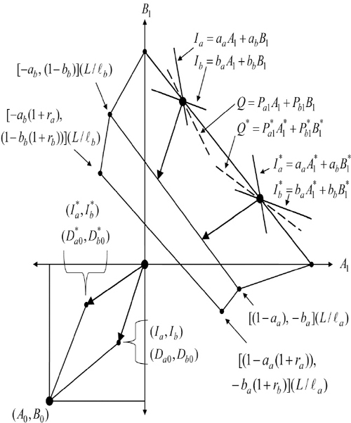
Figure 4.1 From different second period outputs, investment vectors, pointing inward, are shifted to meet first period demand vectors emanating from initial non-storable quantities
two points on the full employment line, connecting L/la and L/lb, show the consequences for (Ia, Ib) of a higher ratio, A1/B1.5 The case considered assumes that aa/ab > la/lb > ba/bb, so that Ia is higher and Ib is lower when A1/B1 is higher. A line corresponding to maximum Q1 = A1Pa1 + B1Pb1 (Garegnani, this volume, n. 24) can cut the labor constraint without violating the condition that relative price should not exceed opportunity cost.6
There is no future beyond period 1, and what is used up in that period is part of the endowment of period 0. However, viability is assumed, with a view to applying the analysis to more general cases (Garegnani, this volume, pp. 35–40). Viability is shown by drawing investment vectors (Goodwin, 1970, p. 25; Walsh and Gram, 1980, pp. 276–80). For each pair of gross outputs, the investment vector (Ia, Ib) points toward corresponding net outputs. The end-points of all such vectors, each beginning at a point on the labor constraint, trace out a full-employment net output schedule.7 This schedule intersects the positive quadrant if and only if (1 − aa)(1 − bb) − abba > 0, the well known viability condition, which is evidently satisfied in Figure 4.1.
Vectors (Ia, Ib) are now shifted to point from the origin in Figure 4.1 into the lower left quadrant, where a box diagram has dimensions defined by the t = 0 endowment, (A0, B0). The requirement for multiple equilibria (see EII, EIII, and EIV in Garegnani’s Figure 1.1) is now clear. If the given points on the labor constraint in our Figure 4.1 are to correspond to a pair of such (E) solutions with positive prices and a positive wage, then the demand vectors at t = 0, emanating from the

Figure 4.2 A price plane shifts inwards as the price of the product Pa1 decreases. A dashed line of possible solutions for input prices W, Pa0 and Pb0 changes position
lower left corner of the endowment box, must be the ones shown.8 The question thus arises as to whether or not this is plausible. Formally, can two input price vectors, (Pa0, Pb0), be found such that the associated wage and output price vectors (W, Pa1, Pb1) induce the two indicated demand vectors, (Da0, Db0) = (A0 − Ia, B0 − Ib) and (Da1, Db1) = (A1, B1)?9 An answer to this question requires analysis of the model’s price relations.
In Figure 4.2, the fixed plane corresponds to good b1 (Pb1 = 1). Any point on it defines input prices (W, Pa0, Pb0) consistent, under competition, with B1 > 0. The variable plane shifts towards the origin as Pa1 is reduced. Any point on it satisfies the competitive price relation for product a1 and is therefore consistent with A1. The planes intersect10 in a line of points (W, Pa0, Pb0) consistent with strictly positive outputs, at a point of intersection of the three constraints in Figure 4.1. In that event, (L, Ia, Ib) are such that a third plane in Figure 4.2, corresponding to minimum Q1 = WL + IaPa0 + IbPb0 (Garegnani, this volume, n. 24), will contain the entire line of intersection of the competitive price planes. By the duality principle of linear programming,
![]()
Figure 4.3 presents the price relations in a way conducive to Garegnani’s argument. His (1.1e) or (1.1f), rewritten as:
![]()

Figure 4.3 A ruled surface shows how the wage measured in terms of b1 varies with own rates of interest ra and rb. The latter two are set equal at the interior dot point: one point on the standard wage—profit curve
![]()
can be solved, after eliminating Pa1/Pb1, to yield the equation for a ruled surface:
| (1) |
Its intersections with two of the three coordinates planes (where W = 0 and rb = −1) define hyperbolic functions whose curvature is determined by the signs of laab − lbaa and abba − aabb (convex to the origin when positive; concave, when negative).11 The surface has a linear intersection with the coordinate plane where ra = −1 (Pa0 = 0). For any other ra, as (1) shows, the inverse relation between W/Pb1 and rb is also linear. In a model in which the real wage is measured in terms of a third good (see Bruno, 1969), points on the surface in Figure 4.3 are intersections of three linearly independent planes, and the surface is no longer ruled.
There is a link between Figures 4.1 and 4.3. Investment vectors corresponding to extreme gross outputs at the end-points of the labor constraint in Figure 4.1 can be multiplied by a uniform profit factor (1 + r) to obtain longer vectors (assuming r > 0) with unchanged slopes. The line connecting their end-points has absolute slope, Pa1/Pb1 = Pa0/Pb0. This case is familiar (Goodwin, 1970, p. 54; Walsh and Gram, 1980, p. 388). When ra ≠ rb, separate Ia and Ib components of the investment vectors emanating from L/la and L/lb, when multiplied by (1 + ra) and (1 + rb), cause those vectors to become shorter or longer, and flatter or steeper, as own rates of interest vary subject to −1 ![]() ra
ra ![]() (1 − aa)/aa and −1
(1 − aa)/aa and −1 ![]() rb
rb ![]() (1 − bb)/bb. The absolute slope of a line connecting the end-points of these adjusted vectors measures:12
(1 − bb)/bb. The absolute slope of a line connecting the end-points of these adjusted vectors measures:12
 |
(2) |
For any given relative price, Pa1/Pb1, own rates of interest are linearly related; in our case, that relation is direct because lbba − labb < 0 and laab − laaa < 0. Note also that:
 |
(3) |
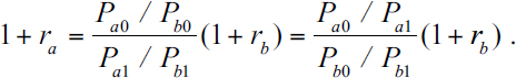 |
(4) |
A line of intersection of price planes in Figure 4.2 (for a given Pa1/Pb1), when intersected in the positive orthant by a vertical plane through the origin (for a given Pa0/Pb0), determines own rates of return (and the real wage in terms of any price).13 Thus, own rates of return are functions of contemporaneous price ratios, as shown by (3) and (4).
Along the ‘main branches’ of Garegnani’s investment and saving schedules, it is assumed that both Pa0 and Pb0 increase, as do ra and rb. In our diagrams, where aa/ab > la/lb > ba/bb, a reduction in Pa1/Pb1 from aa/ab to la/lb causes the line of intersection of price planes in Figure 4.2 to shift in such a way that it may or may not be possible to raise both Pa0 and Pb0.14 However, as Figure 4.3 shows, it is always possible to raise both ra and rb (cf. Garegnani, this volume, p. 46 and n. 10). Thus, a movement along the ‘main branches’ of Garegnani’s investment and saving schedules corresponds, in Figure 4.3 (as W falls), to a movement down the surface in a direction steeper than any line of that surface, and therefore always somewhat in the direction of higher ra.15
Returning to the question of multiple solutions (as indicated in the box diagram in Figure 4.1), we did not succeed in constructing an example to show the type of unstable intersection that occurs at EII and EIV in Garegnani’s Figure 1.1. This may have been a consequence of the numbers chosen for the single technique and/or the form of our utility index. In any case, Garegnani (this volume, p. 23) appears to associate ‘multiple and unstable equilibria’ with the presence of alternative techniques. Choice of technique in an intertemporal equilibrium model is more complex than in a model with uniform own rates of return. If several surfaces (one for each technique) were to be drawn in Figure 4.3 (see also Bruno, 1967, p. 207, and Bruno, 1969, p. 49), their outer envelope could exhibit reswitching at points where ra ≠ rb. Rather than attempting to analyze the relationship between such a complex envelope and Garegnani’s saving and investment schedules, we conclude with some more general remarks.
The traditional long-period equilibrium is characterized by ‘a uniform effective rate of return on the supply prices of the capital goods’ (Garegnani, n. 2). This means that non-uniform own rates of return are consistent with a uniform effective rate of return once changes in relative prices are taken into account. This essential characteristic of the traditional approach is also a central feature of intertemporal equilibrium analysis. Among its first-order conditions are the so-called Euler equations, which state that current yield (own rates of return) plus capital gain or loss (as relative prices change) is the same for all capital goods (Bruno, 1967, eqs. (7) and (49); Burgstaller, 1994, p. 23, n. 10).
Garegnani states that the physical composition of the initial capital stock, if arbitrary, would generally preclude equality of effective rates of return.
In the capital controversies, that inequality of own rates […] has indeed been often confused with the inequality of effective rates on the supply prices of the capital goods, due instead to the unadjusted physical composition of the capital endowment pertaining to Walrasian theory.
(Garegnani, n. 2)
Bruno (1967, 1969) and Burgstaller (1994) and all those whose work they built upon would presumably disagree. The Euler equations do ensure equality of effective rates of return, given an arbitrary physical composition of capital. What they fail to ensure is convergence to a meaningful solution. Transversality and ‘jump’ conditions are also necessary. These are just as damaging for intertemporal general equilibrium analysis, insofar as it constitutes a theory of value, as the required variability of the physical composition of capital is for the coherence of the traditional Walrasian long-period analysis (Garegnani, 1960, pp. 91–119). The reason is that appropriate initial prices must be part of the data (Gram, 2001, pp. 159–60; Burgstaller, 2001, p. 206). Otherwise, changing, but always uniform, effective rates of return will ‘lead to bankruptcy for someone’ (Samuelson, 1967, p. 229). The theory is also bankrupt: ‘A fundamental attribute of Hamiltonian systems is that, as market systems, they are dynamically highly unstable — namely saddle-path stable’ (Burgstaller, 1994, p. 38). This, and not the required variability of the composition of the capital stock in traditional theory,16 is the Achilles heel of intertemporal equilibrium theory. An unstable path cannot provide the foundation for a theory of value and distribution. It is the very antithesis of the classical concept of the long period as a center of gravitation (cf. Burgstaller, 2001, pp. 205–6).
Notes
1 Another relevant paper (Bruno, 1969) was available in July, 1966 as a discussion paper, Department of Economics, Massachusetts Institute of Technology.
2 Robinson offered a prescient warning concerning the mathematical requirements of a formal theory: ‘“The formulae are wiser than the men who thought of them,” and the technique knows a great deal more about the assumptions that it requires than the economist who is expounding it’ (Robinson, 1932, p. 8).
3 This collection includes the paper by Bruno (1967). There is also a candid discussion of the meaning of intertemporal equilibrium by Samuelson (1967, pp. 228–30). His discussion of the required ‘Reaiming Behavior of Speculators’ appears to undercut the entire approach.
4 The possibility of storage is considered by Garegnani, but is not part of his main argument. Therefore, the only way to consume goods in the next period is to produce them. An act of saving is not enough; investment, the actual use of the unconsumed endowment, must occur.
5 The ‘adjustment’ discussed by Garegnani (this volume, n. 24) can be thought of as forcing the three constraints in Figure 4.1 to intersect in a single point. Should either Sa > Ia or Sb > Ib, the corresponding capital good constraint, using the physical component of saving rather than investment, would lie further from the origin. It becomes ‘slack’ or ‘non-binding,’ and its ‘dual’ price, Pa0 or Pb0, falls to zero.
6 Pa1/Pb1 ![]() max (la/lb, aa/ab, ba/bb) and Pb1/Pa1
max (la/lb, aa/ab, ba/bb) and Pb1/Pa1 ![]() max (lb/la, ab/aa, bb/ba) at the two points shown. It is assumed that Pa1/Pb1 is lower when the ratio of quantities demanded, Da1/Db1= A1/Bb, is higher. Think of income consumption paths, corresponding to the two relative price ratios, intersecting the labor constraint at the points shown.
max (lb/la, ab/aa, bb/ba) at the two points shown. It is assumed that Pa1/Pb1 is lower when the ratio of quantities demanded, Da1/Db1= A1/Bb, is higher. Think of income consumption paths, corresponding to the two relative price ratios, intersecting the labor constraint at the points shown.
7 Net outputs corresponding to a given point on the labor constraint would be different if the next period’s gross outputs were to change. Thus, transitional net output schedules differ from steady state net output schedules.
8 A similar diagram could be constructed for different orderings of la/lb, aa/ab, and ba/bb, and/or a more or less productive technique, entailing a larger or smaller value of (1 − aa)(1 − bb) −abba > 0.
9 We note in passing that the Mathematical Note (Tucci, 2000) that accompanies Garegnani (2000) does not impose the requirement that Sa = Ia and Sb = Ib. It is concerned with solutions to system (F) where the weaker requirement, A0/B0 = (Da0 + Ia)/(Db0 + Ib), is imposed.
10 Such a line exists in the strictly positive orthant if and only if Pa1/Pb1 falls within an interval defined by the smallest and largest of the three ratios: la/lb, aa/ab, and ba/bb. In Figure 4.2, this line connects a point in the coordinate plane (Pa0, Pb0) with a point in either the (W, Pa0) plane or the (W, Pb0) plane. The switch occurs as Pa1/Pb1 falls through the intermediate slope la/lb C [aa/ab, ba/bb]. Other cases are similar. Input prices corresponding to the smallest and largest slope of the three lines intersecting at a point in Figure 4.1 define the coordinate plane that will always contain an end-point of the line of intersection of the price planes (when that line exists in the positive orthant). As the contemporary relative price of a1 falls through the value of the intermediate slope of the intersecting constraints in Figure 4.1, the other end-point of the line of intersection switches from one coordinate plane to the other.
11 A second surface with W/Pa1, ra and rb, on the axes would show a line rather than a curve in the plane where rb = −1, and a curve rather than a line in the plane where ra = −1. The latter curve is convex or concave to the origin as balb − bbla is positive or negative.
12 Note that Pa1/Pb1 = la/lb when ra = −1 = rb; Pa1/Pb1 = aa/ab, when rb = −1 and ra = (1 − aa)/aa; and Pa1/Pb1 = ba/bb, when ra = −1 and rb = (1 − bb)/bb.
13 Given Pa1/Pb1 within the interval defined by maximum and minimum ratios, (la/lb, aa/ab, ba/bb), there is a feasible range for Pa0/Pb0 consistent with −1 ![]() rb
rb ![]() (1 − bb)/bb.
(1 − bb)/bb.
14 It will always be possible to do so, as Pa1/Pb1 is reduced, for the case in which la/lb > Pa1/Pb1 > aa/ab > ba/bb. However, as Pa1/Pb1 falls from aa/abto ba/bb in this case, there will necessarily come a point where Pa0 must fall (assuming it is positive at the outset) in order to maintain a non-negative wage.
15 Garegnani’s assumption (iii) that Pa0 and Pb0 always rise together means, in terms of the case shown in our Figure 4.2, that the corresponding increase in Pa1/Pb1 must be sufficiently small (cf. Garegnani, this volume, p. 46, n. 10).
16 Although variability in the composition of the capital stock has, for the most part, been analyzed at the level of the economy as a whole, it was once thought to be a problem at the level of the firm. A well-known standard treatment of price theory contains perhaps the last vestige of this concern (Stigler, 1987[1942], p. 136).
References
Bliss, C.J. (1975). Capital theory and the distribution of income, Amsterdam: North-Holland.
Bruno, M. (1967). ‘Optimal accumulation in discrete capital models’, in K. Shell (ed.), Essays in the theory of optimal growth, Cambridge, MA: MIT Press.
Bruno, M. (1969). ‘Fundamental duality relations in the theory of capital and growth’, Review of Economic Studies 36, pp. 39–53.
Burgstaller, A. (1994). Property and prices: Toward a unified theory of value, Cambridge: Cambridge University Press.
Burgstaller, A. (2001). ‘Some metatheoretical reflections and a reply to critics’, Metroeconomica 52, pp. 197–216.
Burmeister, E. (1980). Capital theory and dynamics, Cambridge: Cambridge University Press.
Cass, D. and Shell, K. (1976). The Hamiltonian approach to dynamic economics, New York: Academic Press.
Dorfman, R., Samuelson, P.A. and Solow, R.M. (1958). Linear programming and economic analysis, New York: McGraw-Hill.
Garegnani, P. (1960). Il capitale nelle teorie della distribuzione, Milano: Giuffrè.
Garegnani, P. (2000). ‘Savings, investment and capital in a system of general intertemporal equilibrium’, this volume, pp. 13–74 (slightly amended version of the paper appeared in H. Kurz (ed.), Critical essays on Piero Sraffa’s legacy in economics, Cambridge: Cambridge University Press).
Goodwin, R.M. (1970). Elementary economics from the higher standpoint, Cambridge: Cambridge University Press.
Gram, H.N. (2001). ‘Critical comments on André Burgstaller’s Property and prices: toward a unified theory of value’, Metroeconomica 52, pp. 149–61.
Hahn, F.H. (1982). ‘The neo-Ricardians’, Cambridge Journal of Economics 6, pp. 353–74.
Malinvaud, E. (1953). ‘Capital accumulation and efficient allocation of resources’, Econometrica 21, pp. 233–68.
Robinson, J.V. (1932). Economics is a serious subject, the apologia of an economist to the mathematician, the scientist and the plain man, Cambridge: W. Heffer and Sons.
Samuelson, P.A. (1967). ‘Indeterminacy of development in a heterogeneous-capital model with constant saving propensity’, in K. Shell (ed.), Essays in the theory of optimal growth, Cambridge, MA: MIT Press.
Samuelson, P.A. and Solow, R. (1956). ‘A complete capital model involving heterogeneous capital goods’, Quarterly Journal of Economics 70, pp. 537–62.
Schefold, B. (1997). Normal prices, technical change and accumulation, London: Macmillan.
Schefold, B. (2000). ‘Paradoxes of capital and counterintuitive changes of distribution in an intertemporal equilibrium model’, in H. Kurz (ed), Critical essays on Piero Sraffa’s legacy in economics, Cambridge: Cambridge University Press.
Shell, K. (ed.) (1967). Essays in the theory of optimal growth, Cambridge, MA: MIT Press.
Sraffa, P. (1960). Production of commodities by means of commodities, prelude to a critique of economic theory, Cambridge: Cambridge University Press.
Stigler, G. (1987 [1942]). The theory of price, 4th edition, New York: Macmillan.
Symposium on Capital Theory (1966). Quarterly Journal of Economics 80.
Tucci, M. (2000). ‘Mathematical note’ to P. Garegnani (2000).
Walsh, V.C. and Gram, H.N. (1980). Classical and neoclassical theories of general equilibrium, New York: Oxford University Press.
REPLY TO GRAM
Pierangelo Garegnani
I am grateful to Professor Gram for the interest he has shown in my essay, and for the attention and time he has devoted to it. I think the diagrams he develops for the model I use are very interesting and may be useful in order to elucidate various steps in the argument and favour a better grasp of it.
I have, however, some comments to make on Gram’s denial that an initial capital endowment given as a physical vector of capital goods — as we have in present-day neoclassical pure theory — precludes uniformity in the effective rate of return1 on the supply prices of such goods. Our disagreement is, however, due to the fact that Gram leaves aside the all-important qualification, present also in the passage of mine he quotes at p. 99, about the rate having to be calculated on the supply prices of the capital goods. He refers instead to the current, or demand, prices of those goods for which the effective rate of return is uniform by the very definition of those prices.2 However temporary the equilibrium we are envisaging, we cannot in fact assume anybody buying a capital good at a price that will not give as high a net rate of return as can be obtained on any other such good. Mere arbitrage will prevent that, and when a capital good happens to be less ‘scarce’ than others, i.e. when its net rental bears a lower proportion to its costs of production, its price will be fixed as a ‘demand price’ below its supply price (cost of production), at the level yielding that higher rate of return. And this is what has to happen for some capital goods when the physical composition of the capital is a given, and cannot therefore be made to suit the outputs and methods of production most profitable in the situation (thus giving rise to different rates of return on their supply prices). Demand prices below supply prices will of course entail that the capital goods in question will not be produced, and that production will be confined to the one or more other capital goods giving the highest rate of return on their supply prices, which will then become the general rate of return on capital.
The problem was in fact a key one for the logical consistency of Walras’s own general equilibrium system. As I have argued at length elsewhere,3 the arbitrary physical composition of his given capital endowment was incompatible with ‘normal prices’ and the corresponding condition of a uniform (effective) rate of return on supply prices, which characterizes those prices and which he, in common with all his predecessors and successors up to recent decades, aimed to determine.4
And the problem exists equally in an intertemporal setting, where, however, it is complicated by the admission of changes in equilibrium prices over time and by the consequent divergence in the same equilibrium situation between the commodities’ own rates of interest, i.e. the rates for loans denominated in different commodities.5 Indeed, the capital controversies of recent decades have been seriously marred by the frequent confusion between, on the one hand, the divergence between own rates and, on the other, the above divergence of effective rates of returns over the capital goods’ supply prices, with which the first has in fact nothing to do: the latter concerns rates of return on the physical capital employed in production, whose relative magnitude is evidently independent of the numeraire adopted, whereas the divergence of own rates concerns merely the numeraire in which a loan (capital) is denominated.
Thus, let the choice of a numeraire, whichever it may be, allow us to have a definite numerical expression for uniform effective return on capital in the given position of the economy. That rate will then emerge in the context of intertemporal prices, just as in the context of Walras’s normal prices, in the price relations (equations or inequalities) of the products, when these are written for undiscounted prices.6 The uniform rate of return appearing there will, however, impose, for the capital goods whose rate of return on costs or supply prices is lower, the ‘demand prices’ that are below the respective supply prices which we saw above. Thus, as in Walras, the divergence of effective rates of return on the supply prices of the capital goods will only show ultimately in the inequality sign of the price relations of these capital goods, whose possibility Gram will readily admit.7
In fact, what happens is that the Walrasian conception of capital forces us to treat as exogenous, an endogenously generated physical composition of the initial capital endowment: this is the essential meaning of the impossibility to satisfy the above condition of uniformity of returns, which in turn entails the impermanence of the resulting equilibria and the undermining of the possibility of correspondence between theoretical and observable variables.
When taken jointly with the drastic impairment that the notion of capital as a vector entails for the possibility of mutual substitution among productive factors,8 the fleeting character of those ‘equilibria’ may easily explain why that Walrasian conception failed to enter the neoclassical mainstream before Hicks (1939), more than a half century after it was first proposed. And even then it could only come to dominate neoclassical pure theory some three decades later, after the first phase of the capital controversies had made untenable the traditional version, based on normal prices and therefore on the conception of the capital endowment as the single magnitude that could take any physical form (Garegnani, 1990, Part II); it is indeed only from then that we can date what I have elsewhere indicated as a deep ‘Hicksian divide’ in the evolution of neoclassical theory.9
We should, however, note that the above criticism of contemporary neoclassicism should be carefully distinguished from the criticism that is central to the essay on which Gram is commenting, and that consists essentially of arguing that the drastic methodological costs paid for the change in the notions of capital and equilibrium appear to have been paid in vain. If the change has eliminated the inconsistent notion of a ‘quantity of capital’ from the highly visible role of expressing the capital endowment, the notion remains nonetheless at the core of the theory in the less visible, but no less basic, role it plays in the market for savings and investment, with essentially the same consequences that have come to light for the traditional versions of the theory.
Notes
1 We qualify the uniformity as relating to the effective rate of return in order to cover the case of multiplicity of own interest rates that the uniformity takes when relative prices change over time (clearly, in an intertemporal equilibrium, the interest rate for a loan denominated in commodity A which rises 1 per cent in price relative to B over the year will have to be 1 per cent lower than the rate on a loan denominated in B.
2 ‘Prix de vente’ is distinguished from ‘prix de revient’, and they are Walras’s terms for our distinction above, translated by Jaffé as ‘selling prices’ and ‘costs of production’, respectively, in his edition of the Elements (1954, par. 247). I have chosen the more familiar Marshallian terms of ‘demand’ and ‘supply’ prices, which seem equally accurate.
3 The point was argued in a 1958 Cambridge Ph.D. thesis and then e.g. in Garegnani (1976) or Garegnani (1990, parr. 11–14).
4 Indeed, Walras himself, once he got over an error affecting, up to the 3rd edition of the Elements, his argument for the existence of a solution to his system, did come to admit this inconsistency. Cf. Garegnani (1976, pp. 103–12).
5 See n.1 above.
6 Cf. Garegnani, this volume, par. 29, n. 8.
7 Thus the inequality sign referred to here, when applied to the price relation for capital goods, has a very different meaning from its applications to consumption goods, where it simply indicates a conceivable good of which nobody is wishing to pay the cost.
8 Garegnani 1990, parr. 49–50
References
Garegnani P. (1976), ‘On a Change in the Notion of Equilibrium in Recent Work on Value: A Comment on Samuelson’, in M. Brown, K. Sato and P. Zarembka (eds), Essays in Modern Capital Theory, Amsterdam, North Holland, pp. 25–45.
—— (1990), ‘Quantity of Capital’, in J. Eatwell, M. Milgate and P. Newman (eds), Capital Theory, London, New Palgrave and Macmillan, pp. 1–78.
—— (this volume, pp. 13–74), ‘Savings, Investment and Capital in a System of General Intertemporal Equilibrium’ (slightly different versions previously published in H. Kurz (ed.) (2000), Critical Essays on Piero Sraffa’s Legacy in Economics, Cambridge, Cambridge University Press, and in F.H. Hahn and F. Petri (eds) (2003), General Equilibrium: Problems and Prospects, London, Routledge.
—— (2005), ‘Capital and Intertemporal General Equilibrium: A Reply to Mandler’, Metroeconomica, 56 (4), pp. 411–37.
Gram H. (this volume, pp. 94–102), ‘Comment on Garegnani’.
Hicks J.R. (1946 [1939]), Value and Capital, London, Macmillan.
Walras L. (1954), Elements of Pure Economics or the Theory of Social Wealth, London, George Allen & Unwin.