
11
Batched Poisson Multirate Elastic Adaptive Loss Models
In this chapter we consider multirate loss models of batched Poisson arriving calls with fixed bandwidth requirements and elastic bandwidth allocation during service. As we have reached the last chapter of the book, the reader should be able to understand the title of this chapter. As a reminder, in the batched Poisson process (in which now a batch consists of two types of calls, elastic or adaptive), simultaneous call‐arrivals (batches) occur at time‐points following a negative exponential distribution. Elastic calls can reduce their bandwidth and simultaneously increase their service time. Adaptive calls can tolerate bandwidth compression without altering their service time.
11.1 The Elastic Erlang Multirate Loss Model with Batched Poisson Arrivals
11.1.1 The Service System
In the elastic Erlang multirate loss model with batched Poisson arrivals (BP‐E‐EMLM), we consider a link of capacity ![]() b.u. that accommodates elastic calls of
b.u. that accommodates elastic calls of ![]() different service‐classes. Calls of each service‐class
different service‐classes. Calls of each service‐class ![]() have the following attributes: (i) they arrive in the link according to a batched Poisson process with rate
have the following attributes: (i) they arrive in the link according to a batched Poisson process with rate ![]() and batch size distribution
and batch size distribution ![]() , where
, where ![]() denotes the probability that there are
denotes the probability that there are ![]() calls in an arriving batch of service‐class
calls in an arriving batch of service‐class ![]() , (ii) they follow the partial batch blocking discipline (see Chapter 10), and (iii) they request
, (ii) they follow the partial batch blocking discipline (see Chapter 10), and (iii) they request ![]() b.u. (peak‐bandwidth requirement). To introduce bandwidth compression in the model, the occupied link bandwidth
b.u. (peak‐bandwidth requirement). To introduce bandwidth compression in the model, the occupied link bandwidth ![]() can virtually exceed
can virtually exceed ![]() up to a limit of
up to a limit of ![]() b.u. Then the call admission is identical to the one presented in the case of the E‐EMLM (see Section 3.1.1).
b.u. Then the call admission is identical to the one presented in the case of the E‐EMLM (see Section 3.1.1).
Similarly, in terms of the system state‐space ![]() , the CAC is expressed as in the E‐EMLM (see Section 3.1.1). Hence, the TC probabilities of service‐class
, the CAC is expressed as in the E‐EMLM (see Section 3.1.1). Hence, the TC probabilities of service‐class ![]() are determined by the state space
are determined by the state space ![]() :
:

where ![]() ,
, ![]() is the number of in‐service calls of service‐class
is the number of in‐service calls of service‐class ![]() in the steady state,
in the steady state, ![]() ,
, ![]() is the steady state probability, and
is the steady state probability, and ![]() .
.
11.1.2 The Analytical Model
11.1.2.1 Steady State Probabilities
The compression/expansion of bandwidth results in a non PFS for the values of ![]() , a fact that makes (11.1) inefficient. In order to analyze the service system and provide an approximate but recursive formula for the calculation of the link occupancy distribution, we assume that local flow balance (as described in Chapter 10) does exist across certain levels that separate two adjacent states of
, a fact that makes (11.1) inefficient. In order to analyze the service system and provide an approximate but recursive formula for the calculation of the link occupancy distribution, we assume that local flow balance (as described in Chapter 10) does exist across certain levels that separate two adjacent states of ![]() . To this end, we present the following notations [1]:
. To this end, we present the following notations [1]:
The first step in the analysis is to define the levels across which local flow balance will hold. For the state ![]() , with
, with ![]() , the level
, the level ![]() separates
separates ![]() from
from ![]() . Then, the “upward” (due to a new service‐class
. Then, the “upward” (due to a new service‐class ![]() batch arrival) probability flow across level
batch arrival) probability flow across level ![]() is given by [ 1]:
is given by [ 1]:

where ![]() , with
, with ![]() , and
, and ![]() is the corresponding steady state probability.
is the corresponding steady state probability.
Equation (11.2) can be also written as follows:

where ![]() is the complementary batch size distribution.
is the complementary batch size distribution.
The “downward” (due to a service‐class ![]() call departure) probability flow across level
call departure) probability flow across level ![]() is given by [ 1]:
is given by [ 1]:
where ![]() , defined according to (3.2), is the common state dependent factor used to compress/expand the service rate of calls, when their bandwidth is compressed/expanded, since the target is to keep constant the product service time by bandwidth per call.
, defined according to (3.2), is the common state dependent factor used to compress/expand the service rate of calls, when their bandwidth is compressed/expanded, since the target is to keep constant the product service time by bandwidth per call.
Due to the compression/expansion mechanism of calls of service‐class ![]() the local flow balance across level
the local flow balance across level ![]() is destroyed, i.e.,
is destroyed, i.e., ![]() or
or

Similar to the E‐EMLM, ![]() are replaced by the state‐dependent compression factors per service‐class
are replaced by the state‐dependent compression factors per service‐class ![]() and
and ![]() which are defined according to (3.8) and (3.9), respectively.
which are defined according to (3.8) and (3.9), respectively.
Having defined ![]() and
and ![]() , we make the assumption (approximation) that the following equation holds:
, we make the assumption (approximation) that the following equation holds: ![]() or
or

Before we proceed with the derivation of a recursive formula for the determination of ![]() , note that the GB equation for state
, note that the GB equation for state ![]() is still given by (10.10). In (10.10), the “upward” probability flows are given by (11.3) and the “downward” probability flows are given by (11.4) (if we refer to
is still given by (10.10). In (10.10), the “upward” probability flows are given by (11.3) and the “downward” probability flows are given by (11.4) (if we refer to ![]() ) or by the RHS side of (11.6) (if we refer to
) or by the RHS side of (11.6) (if we refer to ![]() ).
).
Consider now two different sets of macro‐states: (i) ![]() and (ii)
and (ii) ![]() . For the first set, no bandwidth compression takes place (i.e.,
. For the first set, no bandwidth compression takes place (i.e., ![]() for all
for all ![]() and
and ![]() can be determined by (10.16) [2]). For the second set, ( 11.6) based on (3.8) is written as:
can be determined by (10.16) [2]). For the second set, ( 11.6) based on (3.8) is written as:

where ![]() is the offered traffic‐load of service‐class
is the offered traffic‐load of service‐class ![]() calls (in erl).
calls (in erl).
Multiplying both sides of (11.7) by ![]() and summing over
and summing over ![]() , we have:
, we have:

Due to (3.9), (11.8) is written as:

Let ![]() be the state space where exactly
be the state space where exactly ![]() b.u. are occupied. Then, summing both sides of (11.9) over
b.u. are occupied. Then, summing both sides of (11.9) over ![]() and since
and since ![]() , we have:
, we have:

Interchanging the order of summations in (11.10), we have:

since ![]() .
.
The combination of (10.16) with (11.11) gives the approximate recursive formula of ![]() , when
, when ![]() [ 1]:
[ 1]:

where ![]() is the largest integer less than or equal to
is the largest integer less than or equal to ![]() and
and ![]() is the complementary batch size distribution given by
is the complementary batch size distribution given by ![]() .
.
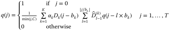
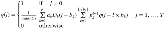
If calls of service k arrive in batches of size ![]() where
where ![]() is given by the geometric distribution with parameter
is given by the geometric distribution with parameter ![]() (for all k) then (11.12) takes the form:
(for all k) then (11.12) takes the form:

If ![]() for
for ![]() and
and ![]() for
for ![]() , for all service‐classes, then we have a Poisson process and the E‐EMLM results (i.e., the recursion of (3.21)).
, for all service‐classes, then we have a Poisson process and the E‐EMLM results (i.e., the recursion of (3.21)).
11.1.2.2 TC Probabilities, CBP, Utilization, and Mean Number of In‐service Calls
The following performance measures can be determined based on ( 11.12):
- The TC probabilities of service‐class
 , via the formula:
(11.14)where
, via the formula:
(11.14)where
 is the normalization constant.
 - The CBP (or CC probabilities) of service‐class
 , via the formula [ 1]:
(11.15)
, via the formula [ 1]:
(11.15)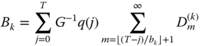
where
 denotes the probability that there are
  calls in an arriving batch of service‐class
  and
and  is the maximum integer not exceeding
  .
.If the batch size is geometrically distributed then (11.15) takes the form:
(11.16)
The proof of (11.16) is similar to the proof of (10) in [3] (which gives the CC probability in the BP‐EMLM where the batch size is geometrically distributed) and therefore is omitted.
- The average number of in‐service calls of service‐class
 , via (3.24), where the values of
  can be determined via:
(11.17)where
can be determined via:
(11.17)where
 and
and  if
if  . The proof of (11.17) is similar to that of (3.25) (see [4]) and thus is omitted.
 - The link utilization, U, via (3.23).
11.2 The Elastic Erlang Multirate Loss Model with Batched Poisson Arrivals under the BR Policy
11.2.1 The Service System
In the elastic Erlang multirate loss model with batched Poisson arrivals under the BR policy (BP‐E‐EMLM/BR) a new service‐class ![]() call is accepted in the link if, after its acceptance, the link bandwidth
call is accepted in the link if, after its acceptance, the link bandwidth ![]() , where
, where ![]() is the BR parameter of service‐class
is the BR parameter of service‐class ![]() .
.
In terms of the system state‐space ![]() and due to the partial batch blocking discipline, the CAC is identical to that of the E‐EMLM/BR (see Section 3.2.1). As far as the TC probabilities of service‐class
and due to the partial batch blocking discipline, the CAC is identical to that of the E‐EMLM/BR (see Section 3.2.1). As far as the TC probabilities of service‐class ![]() are concerned, they are determined by ( 11.1), where
are concerned, they are determined by ( 11.1), where ![]() .
.
The compression factor ![]() and the state‐dependent compression factor per service‐class
and the state‐dependent compression factor per service‐class ![]() are defined according to (3.2) and (3.8), respectively.
are defined according to (3.2) and (3.8), respectively.
11.2.2 The Analytical Model
11.2.2.1 Link Occupancy Distribution
In the BP‐E‐EMLM/BR, the unnormalized values of the link occupancy distribution, ![]() , can be calculated in an approximate way according to the Roberts method (see Section 1.3.2.2).
, can be calculated in an approximate way according to the Roberts method (see Section 1.3.2.2).
Based on Roberts method, ( 11.12) takes the form [ 1]:
where ![]() ,
, ![]() is the largest integer less than or equal to
is the largest integer less than or equal to ![]() ,
, ![]() is the complementary batch size distribution given by
is the complementary batch size distribution given by ![]() , and
, and ![]() is determined via (3.34b).
is determined via (3.34b).
If calls of service ![]() arrive in batches of size
arrive in batches of size ![]() where
where ![]() is given by the geometric distribution with parameter
is given by the geometric distribution with parameter ![]() (for all
(for all ![]() ) then (11.18) takes the form:
) then (11.18) takes the form:
11.2.2.2 TC Probabilities, CBP, Utilization, and Mean Number of In‐service Calls
The following performance measures can be determined based on ( 11.18):
- The TC probabilities of service‐class
 , via the formula [ 1]:
(11.20)where
, via the formula [ 1]:
(11.20)where
 is the normalization constant.
 - The CBP (or CC probabilities) of service‐class
 , via the formula:
(11.21)
, via the formula:
(11.21)
If the batch size is geometrically distributed then (11.21) takes the form:
(11.22)
- The average number of in‐service calls of service‐class
 , via (3.24), where the values of
  can be determined via ( 11.17) assuming that
  when
when  .
. - The link utilization,
 , via (3.23).
11.3 The Elastic Adaptive Erlang Multirate Loss Model with Batched Poisson Arrivals
11.3.1 The Service System
In the elastic adaptive Erlang multirate loss model with batched Poisson arrivals (BP‐EA‐EMLM) we consider a link of capacity ![]() b.u. that accommodates
b.u. that accommodates ![]() service‐classes which are distinguished into
service‐classes which are distinguished into ![]() elastic service‐classes and
elastic service‐classes and ![]() adaptive service‐classes:
adaptive service‐classes: ![]() . The call arrival process remains batched Poisson.
. The call arrival process remains batched Poisson.
The bandwidth compression/expansion mechanism and the CAC of the BP‐EA‐EMLM are identical to those presented in the case of the E‐EMLM (Section 3.1.1). The only difference is in (3.3), which is applied only on elastic calls (adaptive calls tolerate bandwidth compression without altering their service time). As far as the TC probabilities of service‐class ![]() calls are concerned they can be determined via ( 11.1).
calls are concerned they can be determined via ( 11.1).
11.3.2 The Analytical Model
11.3.2.1 Steady State Probabilities
Due to the compression/expansion mechanism of calls of service‐class ![]() the local flow balance across the level
the local flow balance across the level ![]() is destroyed, i.e., (11.5) holds for elastic calls while the corresponding formula for adaptive calls is 5,6:
is destroyed, i.e., (11.5) holds for elastic calls while the corresponding formula for adaptive calls is 5,6:

Similar to the BP‐E‐EMLM, ![]() are replaced by the state‐dependent compression factors per service‐class
are replaced by the state‐dependent compression factors per service‐class ![]() ,
, ![]() and
and ![]() , which are defined according to (3.8) and (3.47), respectively.
, which are defined according to (3.8) and (3.47), respectively.
Having defined ![]() and
and ![]() , we make the assumption (approximation) that the following equations hold:
, we make the assumption (approximation) that the following equations hold: ![]() , or
, or


where the only difference between (11.24) and (11.25) is in ![]() .
.
Before we proceed with the derivation of a recursive formula for the determination of ![]() , note that the GB equation for state
, note that the GB equation for state ![]() is given by (10.10). In (10.10), the “upward” probability flows are given by ( 11.3) and the “downward” probability flows are given by (i) ( 11.5) and (11.23) for elastic and adaptive calls, respectively (if we refer to
is given by (10.10). In (10.10), the “upward” probability flows are given by ( 11.3) and the “downward” probability flows are given by (i) ( 11.5) and (11.23) for elastic and adaptive calls, respectively (if we refer to ![]() ), or (ii) the RHS of ( 11.24), ( 11.25) (if we refer to
), or (ii) the RHS of ( 11.24), ( 11.25) (if we refer to ![]() ).
).
Similar to the BP‐E‐EMLM, we consider two different sets of macro‐states: (i) ![]() and (ii)
and (ii) ![]() . For the first set, no bandwidth compression takes place and
. For the first set, no bandwidth compression takes place and ![]() can be determined by (10.16) [ 2]. For the second set, we substitute (3.8) in ( 11.24) and ( 11.25) to have:
can be determined by (10.16) [ 2]. For the second set, we substitute (3.8) in ( 11.24) and ( 11.25) to have:


where ![]() is the offered traffic‐load of service‐class
is the offered traffic‐load of service‐class ![]() calls (in erl).
calls (in erl).
Multiplying both sides of (11.26a) by ![]() and summing over
and summing over ![]() , we have:
, we have:
Similarly, multiplying both sides of (11.26b) by ![]() and
and ![]() , and summing over
, and summing over ![]() , we have:
, we have:

By adding (11.27) and (11.28), we have:

Based on (3.47), (11.29) is written as:

Summing both sides of (11.30) over ![]() and based on the fact that
and based on the fact that ![]() , we have:
, we have:

By interchanging the order of summations in (11.31), we obtain:

or

because ![]() .
.
The combination of (10.16) with (11.33) gives the approximate recursive formula of ![]() , when
, when ![]() [ 5, 6]:
[ 5, 6]:

where ![]() ,
, ![]() is the largest integer less than or equal to
is the largest integer less than or equal to ![]() and
and ![]() is the complementary batch size distribution given by
is the complementary batch size distribution given by ![]() .
.
If calls of service ![]() arrive in batches of size
arrive in batches of size ![]() where
where ![]() is given by the geometric distribution with parameter
is given by the geometric distribution with parameter ![]() (for all
(for all ![]() ) then (11.34) takes the form:
) then (11.34) takes the form:

If ![]() for
for ![]() and
and ![]() for
for ![]() , for all service‐classes, then we have a Poisson process and the EA‐EMLM results (i.e., the recursion of (3.57)).
, for all service‐classes, then we have a Poisson process and the EA‐EMLM results (i.e., the recursion of (3.57)).
11.3.2.2 TC Probabilities, CBP, Utilization, and Mean Number of In‐service Calls
The following performance measures can be determined based on ( 11.34):
- The TC probabilities of service‐class
 , via ( 11.14).
 - The CBP (or CC probabilities) of service‐class
 , via ( 11.15) or via ( 11.16) if the batch size is geometrically distributed.
 - The average number of in‐service calls of service‐class
 , via (3.24), where the values of
  can be determined via (11.36) for elastic traffic and via (11.37) for adaptive traffic:
(11.36)
can be determined via (11.36) for elastic traffic and via (11.37) for adaptive traffic:
(11.36) (11.37)where
 and
and  if
if  .
. - The link utilization,
 , via (3.23).
11.4 The Elastic Adaptive Erlang Multirate Loss Model with Batched Poisson Arrivals under the BR Policy
11.4.1 The Service System
In the elastic adaptive Erlang multirate loss model with batched Poisson arrivals under the BR policy (BP‐EA‐EMLM/BR) a new service‐class ![]() call is accepted in the link if, after its acceptance, the link bandwidth
call is accepted in the link if, after its acceptance, the link bandwidth ![]() , where
, where ![]() is the BR parameter of service‐class
is the BR parameter of service‐class ![]() .
.
In terms of the system state‐space ![]() and due to the partial batch blocking discipline, the CAC is identical to that of the E‐EMLM/BR (see Section 3.2.1). The only difference is in (3.3), which is applied only on elastic calls. As far as the TC probabilities of service‐class
and due to the partial batch blocking discipline, the CAC is identical to that of the E‐EMLM/BR (see Section 3.2.1). The only difference is in (3.3), which is applied only on elastic calls. As far as the TC probabilities of service‐class ![]() are concerned, they are given by ( 11.1), where
are concerned, they are given by ( 11.1), where ![]() .
.
The compression factor ![]() and the state‐dependent compression factor per service‐class
and the state‐dependent compression factor per service‐class ![]() ,
, ![]() are defined according to (3.2) and (3.8), respectively, while the values of
are defined according to (3.2) and (3.8), respectively, while the values of ![]() are given by (3.47).
are given by (3.47).
11.4.2 The Analytical Model
11.4.2.1 Link Occupancy Distribution
In the BP‐EA‐EMLM/BR, the unnormalized values of the link occupancy distribution, ![]() , can be calculated in an approximate way according to the Roberts method (see Section 1.3.2.2).
, can be calculated in an approximate way according to the Roberts method (see Section 1.3.2.2).
Based on the Roberts method, ( 11.34) takes the form [ 5]:

where ![]() =
= ![]() ,
, ![]() is the largest integer less than or equal to
is the largest integer less than or equal to ![]() ,
, ![]() is the complementary batch size distribution given by
is the complementary batch size distribution given by ![]() , and
, and ![]() is determined via (3.34b).
is determined via (3.34b).
If calls of service ![]() arrive in batches of size
arrive in batches of size ![]() where
where ![]() is given by the geometric distribution with parameter
is given by the geometric distribution with parameter ![]() (for all
(for all ![]() ), then (11.38) becomes:
), then (11.38) becomes:

11.4.2.2 TC Probabilities, CBP, Utilization, and Mean Number of In‐service Calls
The following performance measures can be determined based on ( 11.38):
- The TC probabilities of service‐class
 , via ( 11.20).
 - The CBP (or CC probabilities) of service‐class
 , via ( 11.21) or via ( 11.22) if the batch size is geometrically distributed.
 - The average number of in‐service calls of service‐class
 , via (3.24), where the values of
  can be determined via ( 11.36) and ( 11.37) assuming that
  when
when  .
. - The link utilization,
 , via (3.23).
11.5 Applications
Since the batched Poisson multirate elastic adaptive loss models are a combination of the elastic adaptive multirate loss models (see Chapter 3) and the batched Poisson multirate loss models (see Chapter 10 ), the interested reader may refer to Sections 3.7 and 10.4 for possible applications.
11.6 Further Reading
Similar to the previous section, the interested reader may refer to the corresponding sections of Chapter 3 (Section 3.8) and Chapter 10 (Section 10.5). In addition to these sections, a possible interesting extension could be the recent work of [8]. In [ 8], a self‐optimizing 4G wireless network is considered. The network consists of a group of cells that accommodates elastic and adaptive calls of random or quasi‐random input and incorporates a mechanism for load balancing between the cells of a group. The determination of CBP is based on approximate formulas whose accuracy has been verified via simulation. The case of bursty traffic in such a network could be studied with the aid of the models in this chapter.
References
- 1 I. Moscholios, J. Vardakas, M. Logothetis and A. Boucouvalas, A batched Poisson multirate loss model supporting elastic traffic under the bandwidth reservation policy. Proceedings of the IEEE International Conference on Communications, ICC, Kyoto, Japan, June 2011.
- 2 J. Kaufman and K. Rege, Blocking in a shared resource environment with batched Poisson arrival processes. Performance Evaluation, 24(4):249–263, February 1996.
- 3 E. van Doorn and F. Panken, Blocking probabilities in a loss system with arrivals in geometrically distributed batches and heterogeneous service requirements. IEEE/ACM Transactions on Networking, 1(6):664–667, December 1993.
- 4 S. Racz, B. Gero and G. Fodor, Flow level performance analysis of a multi‐service system supporting elastic and adaptive services. Performance Evaluation, 49(1–4):451–469, September 2002.
- 5 I. Moscholios, J. Vardakas, M. Logothetis and A. Boucouvalas, QoS guarantee in a batched Poisson multirate loss model supporting elastic and adaptive traffic. Proceedings of the IEEE International Conference on Communications, ICC, Ottawa, Canada, June 2012.
- 6 I. Moscholios, J. Vardakas, M. Logothetis and A. Boucouvalas, Congestion probabilities in a batched Poisson multirate loss model supporting elastic and adaptive traffic. Annals of Telecommunications, 68(5):327–344, June 2013.
- 7 I. Moscholios and M. Logothetis, The Erlang multirate loss model with batched Poisson arrival processes under the bandwidth reservation policy. Computer Communications, 33(Supplement 1):S167–S179, November 2010.
- 8 M. Glabowski, S. Hanczewski and M. Stasiak, Modelling load balancing mechanisms in self‐optimizing 4G mobile networks with elastic and adaptive traffic. IEICE Transactions on Communications, E99‐B(8):1718–1726, August 2016.