8.1 The Elastic Engset Multirate Loss Model

8.1.1 The Service System

In the elastic EnMLM (E‐EnMLM), we consider a single link of capacity b.u. that accommodates elastic calls of service classes. Calls of each service class come from a finite source population . The mean arrival rate of service‐class k idle sources is , where is the number of in‐service calls and is the arrival rate per idle source. The offered traffic‐load per idle source of service‐class k is (in erl). Calls of service‐class k request b.u. (peak‐bandwidth requirement). To introduce bandwidth compression in the model, the occupied link bandwidth j can virtually exceed up to a limit of b.u. Then the call admission is identical to the one presented in the case of the E‐EMLM (see Section 3.1.1).

Similarly, in terms of the system state‐space , the CAC is expressed as in the E‐EMLM (see Section 3.1.1). Hence, the TC probabilities of service‐class k are determined by the state space :

(8.1)

where , and .

The compression/expansion of bandwidth destroys reversibility in the E‐EnMLM and therefore no PFS exists (for ), a fact that makes (8.1) inefficient, as Example 8.1 shows.

To circumvent the non‐reversibility problem in the E‐EnMLM, are replaced by the state‐dependent factors per service‐class k, , which have a similar role to and lead to a reversible Markov chain [1,2]. Thus, the compressed bandwidth of a service‐class k call, , becomes (which is (3.7)). To ensure reversibility, have the form of (3.8), where are given by (3.9).

8.1.2 The Analytical Model

8.1.2.1 Steady State Probabilities

The GB equation (rate in = rate out) for state in the E‐EnMLM is given by:

(8.2)

where are the probability distributions of the corresponding states , respectively, which are defined as and , while: and .

Assume now the existence of LB between adjacent states. Equations (8.3) and (8.4) are the detailed LB equations of the modified model (which is reversible):

(8.3)

(8.4)

for and .

Based on the LB assumption, the probability distribution has the solution:

(8.5)

where is the offered traffic‐load per idle source of service‐class k and is the normalization constant given by .

Note that the probability distribution does not have a PFS due to the summation of (3.9) needed for the determination of . We now define , as in (6.26).

Consider now two different sets of macro‐states: (i) and (ii) . For the first set, no bandwidth compression takes place and are determined by (6.27) [3]. For the second set, we substitute (3.8) in ( 8.3) to obtain:

(8.6)

Multiplying both sides of (8.16) by and summing over , we have:

(8.7)

Equation (8.7), due to (3.9) is written as:

(8.8)

Summing both sides of (8.8) over and based on (6.26), we have:

(8.9)

or

(8.10)

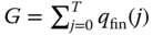
The combination of (6.27) and (8.10) results in the recursive formula of the E‐EnMLM:

(8.11)

8.1.2.2 TC Probabilities, CBP, and Utilization

The following performance measures can be determined based on (8.11):

• The TC probabilities of service‐class k, , via:
  (8.12)
  where is the normalization constant.
• The CC probabilities (or CBP) of service‐class k, , via (8.12) but for a system with traffic sources.
• The link utilization, , via:
  (8.13)

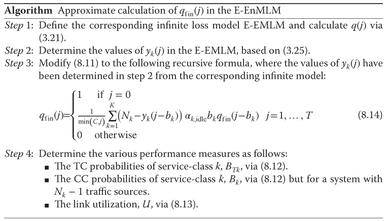
The determination of via ( 8.11) and consequently of all performance measures requires the (unknown) value of (similar to what we have already seen for the proof of (6.27)). To circumvent the complex determination of in each state via an equivalent stochastic system (as already described in Example 6.5), we adopt an approximate algorithm for the calculation of which is similar to the algorithm of Section 6.2.2.3.

8.1.2.3 An Approximate Algorithm for the Determination of

The algorithm comprises the following steps:

8.2 The Elastic Engset Multirate Loss Model under the BR Policy

8.2.1 The Service System

We consider again the multiservice system of the E‐EnMLM and apply the BR policy (E‐EnMLM/BR). A new service‐class k call is accepted in the link if, after its acceptance, the occupied link bandwidth is , where refers to the BR parameter used to benefit calls of other service‐classes apart from k (see also the EMLM/BR in Section 1.3.2).

In terms of the system state‐space , the CAC is expressed as in the E‐EMLM/BR (see Section 3.2.1). Hence, the TC probabilities of service‐class k are determined by the state space :

(8.15)

where , and .

8.2.2 The Analytical Model

8.2.2.1 Link Occupancy Distribution

In the E‐EnMLM/BR, the unnormalized values of can be calculated in an approximate way according to the Roberts method (see Section 1.3.2.2). Based on this, we can either find an equivalent stochastic system (requiring enumeration and processing of the state space) or apply the following algorithm (similar to that presented in Section 8.1.2.3 ):

Note that if for all then the E‐EnMLM results. In addition, if , then we have the EnMLM.

8.2.2.2 TC Probabilities, CBP, and Utilization

The following performance measures can be determined based on (8.16):

• The TC probabilities of service‐class k, , via:
  (8.17)
  where is the normalization constant.
• The CBP (or CC probabilities) of service‐class k, , via (8.17) but for a system with traffic sources.
• The link utilization, , via (8.13).

8.3 The Elastic Adaptive Engset Multirate Loss Model

8.3.2 The Analytical Model

8.3.2.1 Steady State Probabilities

The GB equation (rate in = rate out) for state is given by (8.2) and the LB equations by ( 8.3) and ( 8.4).

Similar to the E‐EnMLM, we consider two different sets of macro‐states: (i) and (ii) . For the first set, no bandwidth compression takes place and are determined by (6.27) [ 4]. For the second set, we substitute (3.8) in ( 8.3) to have:

(8.18a)

(8.18b)

Multiplying both sides of 8.18a by and summing over , we have:

(8.19)

Similarly, multiplying both sides of 8.18b by and , and summing over , we have:

(8.20)

By adding (8.19) and (8.20), we obtain:

(8.21)

Based on (3.47), (8.21) is written as:

(8.22)

Summing both sides of (8.22) over and since , we have:

(8.23)

The combination of (6.27) and (8.23) results in the recursive formula of the EA‐EnMLM:

(8.24)

8.3.2.2 TC Probabilities, CBP, and Utilization

The following performance measures can be determined based on (8.24):

• The TC probabilities of service‐class k, , via ( 8.12).
• The CBP (or CC probabilities) of service‐class k, , via ( 8.12) but for a system with traffic sources.
• The link utilization, , via ( 8.13).

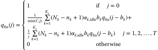
The determination of via ( 8.24) and consequently of all performance measures requires the complex determination of the (unknown) value of in each state j. To circumvent this, we adopt an approximate algorithm for the calculation of which is similar to the algorithm of Section 8.1.2.3 .

8.3.2.3 An Approximate Algorithm for the Determination of

The algorithm comprises the following steps:

8.4 The Elastic Adaptive Engset Multirate Loss Model under the BR Policy

8.4.2 The Analytical Model

8.4.2.1 Link Occupancy Distribution

In the EA‐EnMLM/BR, the unnormalized values of can be calculated in an approximate way according to the Roberts method. Based on this method, we can apply an algorithm similar to that presented in Section 8.3.2.3 , which is described by the following steps:

8.4.2.2 TC Probabilities, CBP, and Utilization

The following performance measures can be determined based on (8.26):

• The TC probabilities of service‐class k, , via ( 8.17).
• The CBP (or CC probabilities) of service‐class k, , via ( 8.17) but for a system with traffic sources.
• The link utilization, U, via ( 8.13).

8.5 Applications

Since the finite multirate elastic adaptive loss models are a combination of the loss models of Chapter 3 and the EnMLM of Chapter , the interested reader may refer to Sections 3.7 and 6.5 for possible applications.

In what follows, we continue the discussion started in Section 3.7 by considering the applicability of the models under SDN technology with the advanced 5G features of Cloud‐RAN (C‐RAN) and the self‐organizing network (SON). The latter enables more autonomous and automated cellular network planning, deployment, and optimization [6]. The considered reference architecture which is appropriate for the applicability of the models is presented in Figure 8.13.

This is in line with the C‐RAN architecture, although it can also support a more distributed, mobile edge computing (MEC)‐like functionality, by incorporating, e.g., the SON features. At the RAN level, the architecture includes an SDN controller (SDN‐C) and a virtual machine monitor (VMM) to enable NFV. Three main parts are distinguished: a pool of remote radio heads (RRHs), a pool of baseband units (BBUs), and the EPC. The RRHs are connected to the BBUs via the common public radio interface (CPRI) with a high‐capacity fronthaul. The BBUs form a centralized pool of data center resources (denoted as C‐BBU). The C‐BBU is connected to the EPC via the backhaul connection. To benefit from NFV, we consider virtualized BBU resources (V‐BBU) where the BBU functionality and services have been abstracted from the underlying infrastructure and virtualized in the form of VNFs [7]. To realize the virtualization, the VMM manages the execution of BBUs. Finally, the SDN‐C is responsible for routing decisions and configuring the packet forwarding elements [8]. Among the BBU functions that could be virtualized in the form of a VNF, we focus on the RRM, which is responsible for CAC and RRA. Various bandwidth/resource sharing policies such as the CS, the BR or the TH could be implemented at the RRM level and enable sharing of V‐BBU resources among the RRHs [9]. An analytical framework for the case where all RRHs in the C‐RAN form a single cluster can be found in [10]. The analysis for the multi‐cluster case is similar and is proposed in [11]. In both [ 10] and [ 11], the C‐RAN accommodates Poisson arriving calls of a single service‐class under the CS policy. Guidelines for the extension of the models of [ 10] and [ 11] in the case of multiple service‐classes are provided in [ 9]. These guidelines could be the springboard for the analysis of elastic adaptive service‐classes of random or quasi‐random input under the assumption that each RRH has subcarriers which can be virtually exceeded up to subcarriers. The latter is essential in order to include the compression/expansion mechanism for elastic adaptive calls.

We continue with the use of SON technology for the implementation of bandwidth/resource sharing policies (and consequently of the multirate loss models). As an implementation example consider a virtualized RRM function in the C‐RAN of Figure 8.13. Traditionally, SON functions refer to self‐planning, self‐optimization, and self‐healing. Implementing the RRM function as a SON function would mainly target the self‐optimization objective, although this could also greatly facilitate the self‐planning objective. In particular, the goal of self‐optimization is as follows. During the cellular network operation, self‐optimization intends to improve the network performance or keep it at an acceptable level. The optimization could be performed in terms of QoS, coverage, and/or capacity improvements and is achieved by intelligently tuning various network settings of the BS as well as of the RRM function (e.g., CAC thresholds and RRA parameters). In the literature, the following architectural approaches for implementing the SON functions have been proposed [ 6]:

1. Centralized SON (cSON): the SON functions are executed at the network management system (NMS) level or at the element management system (EMS) level. This will be particularly suitable for highly centralized C‐RAN solutions.
2. Distributed SON (dSON): the SON functions are executed at the BS level. They can be implemented either within a BS or in a distributed manner among cooperating BSs. This is beneficial for scenarios that require pushing the network intelligence closer to MUs.
3. Hybrid SON (hSON): a combination of cSON and dSON concepts (as shown in Figure 8.14). According to this approach, some SON functionality is distributed and executed at the BS level, whereas other SON functionality is centralized at the NMS or EMS level.

Policies such as the CS, BR or the TH (described in this book), although they can be used under all three approaches, may have most benefit under the hSON. Focusing on SON's self‐optimization function, we consider the optimization of CAC. The CAC function (part of the dSON) admits or rejects a call, while the cSON function performs the selection of the optimization parameters for the CAC algorithm. These parameters are, for example, the BR parameters. In fact, the BR parameters can be used not only for CAC, but also for determining the allocated bandwidth to calls of each service‐class. When the cSON selects the CAC optimization parameters, it considers the overall resource utilization in the cell, the QoS requirements of already accepted calls, and the requirements of the new call. According to the selected bandwidth/resource sharing policy (e.g., the BR policy), its corresponding parameters (e.g., the BR parameters) are sent from the cSON to the dSON/RRM. The cSON sends an updated set of parameters if any changes in the performance guarantees are required (e.g., different acceptable levels of CBP). In the simplified case (e.g., when operating under tight resource or energy constraints) only the current values of the parameters are sent to the dSON/RRM. In particular, the cSON determines the configuration parameters based on a number of objectives (e.g., acceptable CBP). The dSON at the RAN receives the configuration parameters and acts accordingly (e.g., rejects connection requests that do not conform to the specified parameters). If the measurements reported from the dSON to the cSON violate the objectives (e.g., the CBP for a particular service is too high), the cSON will re‐calculate and send updated configuration parameters to the dSON. This approach can result in a more autonomous and automated cellular network functionality and enables simpler and faster decision‐making and operation.

8.6 Further Reading

Similar to the previous section, the interested reader may refer to the corresponding sections of Chapter 3 (Section 3.8) and Chapter 6 (Section 6.6) in order to study possible extensions of these models.

References

1. 1 V. Koukoulidis, A Characterization of Reversible Markov Processes with Applications to Shared‐Resource Environments, PhD thesis, Concordia University, Montreal, Canada, April 1993.
2. 2 V. Iversen, Reversible fair scheduling: The teletraffic theory revisited. Proceedings of the 20th International Teletraffic Congress, LNCS 4516, pp. 1135–1148, Ottawa, Canada, June 2007.
3. 3 G. Stamatelos and J. Hayes, Admission control techniques with application to broadband networks. Computer Communications, 17(9):663–673, September 1994.
4. 4 I. Moscholios, J. Vardakas, M. Logothetis and M. Koukias, A quasi‐random multirate loss model supporting elastic and adaptive traffic. Proceedings of the 4th International Conference on Emerging Network Intelligence, EMERGING 2012, Barcelona, Spain, September 2012.
5. 5 I. Moscholios, J. Vardakas, M. Logothetis and M. Koukias, A quasi‐random multirate loss model supporting elastic and adaptive traffic under the bandwidth reservation policy. International Journal on Advances in Networks and Services, 6(3&4):163–174, December 2013.
6. 6 Self‐Organizing Networks (SON); Concepts and Requirements (Release 12), document 3GPP 32.500 v12.1.0, September 2014.
7. 7 Network Function Virtualisation (NFV); Management and Orchestration, document ETSI GS NFV‐MAN 001 (V1.1.1), December 2014.
8. 8 T. Chen, M. Matinmikko, X. Chen, X. Zhou, and P. Ahokangas, Software defined mobile networks: Concept, survey, and research directions. IEEE Communications Magazine, 53(11):126–133, November 2015.
9. 9 I. Moscholios, V. Vassilakis, M. Logothetis and A. Boucouvalas, State‐dependent bandwidth sharing policies for wireless multirate loss networks. IEEE Transactions on Wireless Communications, 16(8):5481–5497, August 2017.
10. 10 J. Liu, S. Zhou, J. Gong, Z. Niu, and S. Xu, On the statistical multiplexing gain of virtual base station pools. Proceedings of IEEE Globecom, Austin, TX, USA, December 2014
11. 11 J. Liu, S. Zhou, J. Gong, Z. Niu, and S. Xu, Statistical multiplexing gain analysis of heterogeneous virtual base station pools in cloud radio access networks. IEEE Transactions on Wireless Communications, 15(8):5681–5694, August 2016.