Chapter 3

Statistical Behavior of Stirred Waves in an Oversized Cavity

3.1. Introduction

Chapter 2 reached the conclusion that the field distribution observed in an electromagnetic cavity was hard to predict when its dimensions were much higher than the wavelength. The theoretical difficulty mainly comes from the presence of scattering devices. We can add to these geometrical details the energy losses. Their contribution manifests itself in the appearance of groups of modes, whose relative intensity depends on the lesser displacement of the transmitting antenna immersed in the chamber. If the calculation of the field remains possible using theoretical simulations adapted to the context of the MSRC, the use of these numerical models is extremely costly in computer resources. All of these reasons have thus encouraged scientists to compare the electric or magnetic fields with random variables. We will try to add to these variables probability density functions and statistical properties, all examined in this chapter [KOS 91, SER 09].

Section 3.2 is devoted to the statement of the postulate specifying that the distributed field in a perfect MSRC answers to the largest random behavior. This means that under continuous sinusoidal excitation, the complex components of electric (or magnetic) field variable appropriate the conditions of maximum entropy and minimum energy. This reasoning leads to the normal probability density function (pdf), while assuming an isotropic field distribution. Thus, the complex components of the electric field vector (or of the magnetic field vector ) give six centered random variables, which are assumed to be independent and to possess the same standard deviation. Knowing that the sensors or receiving antennas generally only measure the absolute amplitudes of these field components or a power proportional to their square amplitudes, the Rayleigh probability distribution and the exponential distribution result from these properties. The calculations of the moments of these variables will be undertaken and presented with specific notation conventions.

Section 3.3 is entirely devoted to the simulation of an ideal random field. This is not about exactly reproducing the field distribution found in an actual reverberation chamber, but about supplying amplitude data respecting the previously stated Rayleigh or exponential distributions. The process consists of using the properties of the plane wave spectra developed in Chapter 2. With the help of pseudo-random generation of these random variables draws, we will show that the field coming from such a simulation is wreathed with uncertainties. These uncertainties can be quantified thanks to the joint applications of the large numbers law and of the central limit theorem (CLT).

Section 3.4 goes into depth on the subject of the statistical concepts previously stated. It is about comparing the experimental data to the probability density distributions resulting from the ideal random field. We then use the estimate of the mean amplitudes and the variances. They will be the subject of some theoretical considerations. The analysis will then turn to the use of the statistical Kolmogorov-Smirnov test (or KS test). The application of this test seems quite appropriate to the context of the reverberation chambers. Theoretical simulations and comparisons to experimental data will conclude this section.

Section 3.5 is more particularly devoted to the use of statistical properties, in order to determine the balance of the powers observed between a transmitting antenna and a receiving antenna, both installed in the room. These features will be used to define a measurement procedure of the transmitting power of a device, as well as to determine the composite quality factor of the chamber.

3.2. Descriptions of the ideal random electromagnetic field

3.2.1. The electromagnetic field assumed as a random variable

Let us consider a reverberation chamber containing a mode stirrer and a transmitting antenna connected to a source of sinusoidal signals of angular frequency ω₀. This angular frequency is assumed to be much higher than the minimum angular frequency ω_s. The latter marks the boundary of the expected functioning of the chamber. By the expression “expected functioning”, we mean the physical feature of the field distribution corresponds f to the behavior of random variables with regards to the powers and voltages collected by a device. Generally, the angular frequency or the lowest frequency represents five or six times the angular frequency or the first eigenmode frequency of the chamber. For the illustration adopted in this chamber, the first eigenmode angular frequency will be designated by the symbol ω₀₁₁. Readers interested in knowing the definition of the angular frequencies or the first eigenmode frequencies of a rectangular shaped cavity can refer to section 2.3.3 of Chapter 2. The position of the ω₀ angular frequency of the expected functioning consequently meets the criteria below:

[3.1]

Since the electromagnetic field is established in a chamber with high but finite conductivity walls after an initial transient response, we reach the continuous sine wave of the fields under the ω₀ angular frequency. If we first take a look at the electric field, using the complex numbers, the function identified with the lower case e will depend on three space variables, x, y, z and on the time variable t. The electric field can be polarized according to one of the three directions of the Cartesian graph. We will thus use the convention of e_x,y,z indices. The electric field complex function in any point of the chamber, will thus be presented by equation [3.2], where the use of the capital letter in E_x,y,z is aimed at the complex amplitude function reduced to just the space variables:

[3.2]

Let us recall that under these notations, the physical signal corresponds to the real part of the complex function in equation [3.2].

The E_x,y,z function can also be projected under a Cartesian form where the real and imaginary component, will be associated with r and j superscripts:

[3.3]

To avoid overloading equation [3.3], the x, y and z space variables have not been recalled. The functions that represent the real and imaginary components of each Cartesian projection of the field E_x,y,z are therefore real random numbers. The latter are quantities that we will be merged into the random dummy variable designated by ν. This means that we establish between ν and the previous functions, the correspondence rules shown below:

[3.4]

From the physical point of view, the v variable describes the rms amplitude of one of the two components of the E_x,y,z(x, y, z) function; this is for an observer located at any point inside the chamber. In practice, this data will be supplied by measurement sensors of the electric field or by numerical simulations. We can thus have very large samples of the v amplitudes and v will be assumed to be a random variable. We propose to add to this variable a probability density function (pdf) taking the usual p(ν) notation. This pdf obviously fulfills the normalized integral [3.5]:

[3.5]

This unbounded integral assumes that ν occupies an infinite set of values. This is obviously incorrect, since the fields amplitude is naturally limited by the finite amplitude of the standing wave that results, from energy losses. We will come back to this matter in other parts of this section. We make the assumption that the random behavior of the amplitude of the real or imaginary component of the field does not favor any polarity and that the linear functioning gives to ν (i.e. to the field components) a balanced distribution around the null mean value. Consequently, the computation of the moment of ν leads to a centered variable. This feature translated in the usual notations of the probability theory recalled in Appendix 1 is expressed by relationship [3.6]:

[3.6]

We add to this first property, the postulate meaning that the distribution of the v variable is independent from the field polarization. In other words, the variances of the v variables are all identical to a same value designated by the conventional symbol. This postulate transposed in equation [3.7] features the isotropy of the field distribution:

[3.7]

It thus remains to seek a probability distribution p(ν), known to be compatible with the experimental facts or in agreement on idealized physical properties. The first process consists of gathering data collections, in order to build histograms that we will compare to theoretical distributions. The second method is based on the statement of a hypothesis aimed at idealizing the statistical features of the expected experimental pieces of data. These properties will be compared to tests, in order to check the agreement with the experiment. In section 3.2.2 we will use the second method and recall its theoretical foundations.

3.2.2. Statement of the postulate of an ideal random field

The postulate was initially formulated in an article from D.A. Hill published in 1998. It states that the amplitudes of a very large sample of v variables collected in a reverberation chamber are distributed in a perfect random manner [HIL 98]. According to the principle of Boltzmann’s statistics, the ideal statistical properties of the variable v satisfy the state of minimum u energy and of maximum S entropy. The energy is linked to the square amplitude of ν weighted by the a physical unit coefficient U₀. The entropy is defined by the product of Boltzmann’s constant k_B and of the natural logarithm of the p(ν) probability density function attached to the v variable, i.e.:

[3.8]

Equation [3.8] enables us to formulate the criteria of minimum energy and maximum entropy by calculating the first derivatives:

[3.9]

After using Lagrange multipliers, we reach the differential equation presented below:

[3.10]

In this equation, the K coefficient includes all the previously introduced constants.

The solution of equation [3.10] is an exponential decreasing function in which the square of the variable v appears:

[3.11]

After the calculations of the moment of ν² and of the normalized integral of p(ν) given in [3.5], we easily manage to connect the A and K unknown constants to the standard deviation and to the variance of the v variable. The p(ν) function then takes the definitive form of the normal probability density distribution. To designate pdf of the normal distribution, we use the p_n symbol — the letter n recalls that we aim for a normal distribution:

[3.12]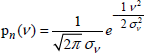

The standard deviation σ_ν that is the square root of the variance features the scattering of the v variable around zero. This scattering will depend on the physical properties of the chamber, notably on the quality factor and on the direct couplings exerted by antennas or devices. We will see in Chapter 8 that the contribution of direct couplings leads to the collected field data in the room tends to move away from the normal distribution formulated by equation [3.12].

We will see in the following of this section that we use normalized variables as well as variables other than v. Section 3.2.3 is devoted to the conventions adopted for the definitions of these new variables.

3.2.3. Presentation conventions of the random variables

3.2.3.1. Absolute amplitude of the electric field

Most of the electric field probes used in test chambers give a voltage proportional to the absolute amplitude of the complex electric field E_x,y,z.

Consequently, this variable modulus will be defined and presented with the writing conventions of equation [3.13]:

[3.13]

Generally, the output data of the field sensors is a voltage proportional to the amplitude of one of the x, y, z projections of the field vector.

3.2.3.2. Power collected on an antenna

If we admit that the antennas are polarized according to one of the three electric field projections, the power variable designated by the p symbol is linked to the square of the electric field amplitude times a physical unit factor A₀. To avoid the mix-up with the probability density symbol, the p power variable will be written in italics:

[3.14]

We will note that this formula can also concern the power detected at the output of a field probe connected on a load resistance.

3.2.3.3. Normalized field and power variable

To ease some demonstrations or to lighten the presentation of some results, we frequently use the normalized variable concept. We successively distinguish the normalized variable v_r attached to the components of the complex electric field, the normalized power p_r collected by an antenna and the normalized variable of the absolute electric field amplitude e_r. The v_r variable will be made up of the ratio linking the v variable to its standard deviation σ_v:

[3.15]

Using the transformation suggested below, we easily move from the normal distribution attached to the v variable to its equivalent distribution associated wtih the normalized variable v_r:

[3.16]

We easily take from this equation the expression of p_n(v_r), hence:

[3.17]

The normalized variable p_r comes from the ratio linking p to its mean value p_mv, i.e.:

[3.18]

This mean value is the first moment of p:

[3.19]

However, calculation of the expected value assumes prior knowledge of the pdf of the p variable. This question will be resolved in the next section.

3.2.3.4. The χ² variable

The square electric field amplitude appears in the definition of the power variable given in [3.14]. This amplitude can be written with the normalized form of the v variable taken from relationship [3.15]. The result will be presented in equation [3.20], where we can find the v₁ and v₂ auxiliary variables. They are respectively linked to the real and imaginary components of E_x,y,z formulated below:

[3.20]

The χ² normalized variable will thus be defined by the sum of the square amplitudes of v₁ and v₂, i.e.:

[3.21]

3.2.3.5. Normalized absolute amplitude of the electric field

The normalized absolute amplitude of the electric field is given by the square root of the χ² variable, which is the ratio of the field modulus expressed in [3.13] and of the standard deviation of the v variable. This absolute amplitude will be designated by the lower case e with the index r:

[3.22]

3.2.4. χ² probability distribution

Let us consider a set of n centered and normalized random variables x_i, each attached to a normal probability distribution. This sample forms a χ² variable with n degrees of freedom, expressed as follows:

[3.23]

We can show that under these conditions, the α variable designated in the previous equation leads to the χ² distribution formulated below [BAS 67, PAP 91]:

[3.24]

In this formula the Eulerian function Γ(s) is described by the integral:

[3.25]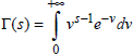

The pdf of the χ² distribution will be used in the next sections, in order to find probability distributions of the absolute electric field amplitude and of the power variable.

3.2.5. Probability density function of the absolute field amplitude

According to equation [3.22], the normalized absolute amplitude of a field projection is the square root of the χ² variable with two degrees of freedom. Consequently, the corresponding probability density function can be determined by the χ² distribution [3.24], for n = 2, i.e.:

[3.26]

The index 2 at the bottom of the p symbol recalls that we aim for two degrees of freedom. We then go from the dummy variable α to the normalized variable e_r of the absolute field amplitude with the help of the following transformation:

[3.27]

We easily take from this relationship the e_r probability density function:

[3.28]

The R index at the bottom of the p symbol indicates that it is Rayleigh’s distribution. The definitions introduced in appendix 1 easily lead to the moments computation of the e_r variable, i.e.:

— first moment:

[3.29]

— second moment:

[3.30]

After insertion of the absolute field value coming from relationship [3.22], the pdf of the absolute amplitude of E_x,y,z becomes:

[3.31]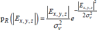

By combining relationships [3.22] and [3.29], we reach the mean value of the absolute amplitude of one of the electric field projection, i.e.:

[3.32]

The mean value (i.e. the first moment of the underlying distribution) amplitude term is adopted, contrary to the estimated mean amplitude (over a finite sample of measured data) widely used in other parts of the book.

3.2.6. Probability density function of the power variable

The probability density function of the p power variable comes from equation [3.26] that we seek to formulate in the writing of [3.33]:

[3.33]

After some algebraic calculations, we reach relationship [3.34] in which we link the p_mv parameter to the coefficient of the A₀ physical scale, and to the variance of the ν variable:

[3.34]

We find the exponential probability distribution. The index 2 at the bottom of the p symbol recalls that the function comes from the χ² variable with two degrees of freedom. We will see in Appendix 3 that pdfs [3.31] and [3.34] can be extended to the total electric field vector, as well as to the total power coming from the isotropic composition of the three projections of the complex components of the electric field vector.

Let us specify that p_mv is the first moment of the p variable, i.e. the expected value of the p variable given by:

[3.35]

We easily deduce from expression p₂(p), the pdf of the p_r normalized power variable, i.e.:

[3.36]

It is important to note that the variables entering the Rayleigh and exponential formulas are all positive real numbers and that, as such, the formulas should contain the step function. This function has not been mentioned, in order to simplify the writing of the equations.

3.3. Simulation of the properties of an ideal random field

The research of an ideally random field distribution is the required condition for the normal use of a reverberation chamber. Indeed, if we justify by adequate calibration processes that the pdfs remain stationary, we can reach the conditions leading to reproducible experiments.

The evaluation of the stationary state can only be carried out with the help of the statistical estimators stated in section 3.4 of this chapter. Therefore, we first take a look at the implementation of the simulations of resulting field interference with ideal statistical properties.

The last part of section 3.3 will thus be entirely devoted to this task, based on the use of plane wave interferences randomly distributed in the space. We will see that the development of these waves gives access to the main statistical parameters enabling us to observe the stationary state criteria.

3.3.1. Construction of the plane wave spectrum

Let us briefly come back to the plane wave spectrum introduced in section 2.3.6 and more especially to Figure 2.14, in which we find the positions of the wave numbers attached to the excitation of the TM₃₃₃ mode.

Considering this is based around an empty cavity, it appeared that the electric field transformation in the space of the wave numbers led to a cluster of eight points symmetrically positioned at the corners of a parallelepiped. The latter is centered at the origin of the wave numbers graph.

It is thus easy to conclude from the geometrical representation that the TM₃₃₃ mode amounts to the interference of eight plane waves, whose incidence angles are indeed specified by the coordinates of each of these eight points. In accordance with the electric field configuration found on the TM₃₃₃ mode, the calculation only concerns the E_z polarization. A point of the diagram of the wave numbers can thus be reproduced by a plane wave to which we add a representation borrowed from the algebra of the complex numbers.

To go into more details, let us consider the oxyz coordinate system presented in Figure 3.1, i.e. an o’ point to which we attach the wave number vector . This vector belongs to a plane wave of any incidence brought back to the solid angle Ω and to an amplitude E_w attached to the vector.

By taking into account the conventions adopted in this figure, the wave number vector has three projections designated by the k_x, k_y, k_z symbols that we easily link to the unit vectors, shown on the graph by equation [3.37]:

[3.37]

Knowing that it is more convenient to project the Ω incidence angle of the wave in a spherical graph, the θ polar coordinate and the φ azimuthal coordinate have been added to this diagram. It is clear that each of these three projections of the vector can be expressed by the formulas in [3.38], in which the θ and φ variables appear:

[3.38]

The polarization plane of the wave is perpendicular to the o’o propagation direction, maintained by the wave number vector . Thus this property reduces the vector to two components projected on the o’θ and o’φ axes recalled on the left of Figure 3.1. The polarization angle of the wave defined by the η symbol is thus linked to the E_wθ and E_wφ components of by the following expressions:

[3.39]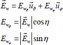

Let us consider an observer marked at any point of the space by the vector defined below:

[3.40]

We propose building the complex expression of the plane wave by adopting, as a phase reference, the position that the wave will have at the origin of the oxyz coordinate system. Under this condition and taking into account the structure of the wave number vector found in the equations in [3.39], the electric field vector will be a function of the position vector formulated in expression [3.41]. The constitution of this formula calls upon the presentation conventions of the plane wave described in section 1.1 of Chapter 1:

[3.41]

Under these notations, the _w(0) vector projected on the coordinates x, y, z, thus directly expresses the amplitude and the polarization of the wave at the origin o of the graph. Let us specify that by a combination of axes’ rotations, we go from the spherical projections of established by [3.39] to the three Cartesian projections.

For example, the E_wz component projected on the oz axis is expressed by relationship [3.42] below:

[3.42]

The reasoning can easily be extended to the magnetic field vector contained in the polarization plane of the wave, orthogonal to .

From examining the diagram of the wave numbers and of the plane wave described by [3.41], we can formulate some hypotheses on the way to stimulate an ideal random field. Figure 2.14 from Chapter 2 shows that the stationary wave attached to the TM₃₃₃ mode produces in the space perfectly ordered eight point wave numbers where the o graph origin of the vectors is a center of symmetry.

Transposed to the context of Figure 3.1, the stationary wave results from the interference of the eight plane waves with strictly similar amplitudes, whose incidence angles are rigorously symmetrical. The resulting wave then brings about an electric field polarized according to the oz axis of this figure.

Reproducing a completely perfect random field can consist of breaking off the diagram symmetry in the space of the vectors. This comes down to distributing the points by following a random cluster within two concentric spheres, which are infinitely close together. Their radius is the k norm of the vector.

This norm is thus imposed by the f₀ excitation frequency of the chamber, i.e.:

[3.43]

According to this assumption, the unit vector carries the radial direction of the waves, whereas the Δk spacing of the radii of the infinitely close together spheres comes from the Δf₀ bandwidth. The latter is generated by the quality factor of the chamber.

If we return to equations [3.38] and [3.39], we can notice that we have four degrees of freedom in order to build an ideal random field from the interferences of N^th plane waves. We successively count the Ω solid incidence angle including the θ and φ variables, the η polarization angle and the E_w amplitude of the wave. Even if this parameter has not yet already been mentioned, we must add the phase angle α of the continuous sinewave brought back to the transmitting antenna.

The Ω, η and α variables are respectively bounded in the limits [0 4π] for Ω, [0 2π] for η and [0 2π] for α. Thus, these restricted domains lend themselves quite well to the practice of random realizations carried out on a uniform distribution of random numbers. The E_w amplitude term does not offer this convenience. We propose to maintain it as an invariant. This hypothesis thus amounts to transferring the random behavior of E_w on the Ω incidence angle of the theoretically ordered wave.

We will indeed show in the next section that the complex field resulting from the interference of a large number of plane waves - with invariant amplitudes, and with incidence angle Ω, polarization angle η and phase angle α, all randomly drawn — produces a resulting field with an ideal random distribution according to the normal probability distribution.

3.3.2. Construction of the interferences by random trials

The construction of interferences described in the previous section amounts performing Monte Carlo simulations draws, generated by a random variable u, uniformly distributed in the [0 +1] interval [LAD 99, MUS 03].

The index i, found on the variables with incidence angle Ω_i, polarization angle η_i and phase angle α_i, designates the wave of row i of the set N. The link with the u variable is made using the equations in [3.44] below:

[3.44]

Let us specify that in the notation conventions of the right members of equation [3.44], the indices added to the u independent variables determine the physical reference parameter and the i index at the bottom of the brackets designates the row of the trial.

From the diagram in Figure 3.1, we know that the solid angle is projected on the φ and θ coordinates of the spherical graph. Thus, the polar angle θ_i and the azimuth angle φ_i must correspond to the trial of the u variable found in relationship [3.44] brought back to the solid angle Ω_i. Knowing that the projection of o’ on the polar axis is the cosine of the θ_i, variable, this criterion means that the numerical values of u necessarily enter within the bounds of the cosine function, i.e. the [−1 +1] interval. Formula [3.45] consequently establishes the link between the random values of u and cos θ_i:

[3.45]

Determination of the value allocated to the φ_i variable describing the azimuthal projection of the solid angle is easier, because it is reduced to the product of u by 2π, hence:

[3.46]

The random variable of phase α_i is inserted according to the polar notation of the complex amplitude of E_w, i.e.:

[3.47]

After insertion of the polar angle and the polarization angle mentioned in equation [3.42], the E_wz field carried by the wave of row i will be presented as follows:

[3.48]

The simulation consists of calculating the resulting field determined by the algebraic sum of the set of N amplitude terms mentioned in [3.49]:

[3.49]

Let us recall that the r and j indices set in superscript indicate that we aim for real and imaginary components of the field. Continuing the demonstration consists of calculating the first moment and the variance of the two terms of series [3.49]. We produce the calculation of the imaginary component, because the reader can easily extend it for the real one.

Each term of the imaginary component of the series can be represented by the product of the absolute field amplitude |E_w| and of three random variables designated by the v_α, v_η, v_θ symbols. These auxiliary variables will be connected to the geometrical variables of the plane wave θ_i, η_i, and α_i, with the following:

[3.50]

Knowing that the sinus and cosine functions evolve symmetrically compared to the zero value, this is about random centered variables. This property can thus be extended to the v_α, v_η, v_θ auxiliary variables.

The random trials carried out to determine the numerical values of the polar angle and the phase and polarization angles are independent. We thus reach the conclusion that v_α, v_η, v_θ are also independent variables.

It results from these considerations that the mean value of the amplitude of the imaginary field component is deduced from the product of the variances of the three v_α, v_η, v_θ variables. The calculation of the expected value will thus require the research of three probability density functions taking as respective symbols: p_α(v_α), p_θ(v_θ) and p_η(v_η). We will carry out the demonstration leading to the p_α(v_α) and p_θ(v_θ) functions. We can easily extend it to p_η(v_η).

The inversion of the previously established functions, followed by the combination with the initial formulas [3.46] gives three expressions of u. Later on we will look for the first derivatives of u:

[3.51]

By carrying out the calculation of the differential du, we manage to identify this variable with the elementary probability density dp_i. The i index at the bottom of the p symbol will correspond to the index found at the bottom of the v variables, attached to each one of the three equations in [3.51]. For example, for the first equation containing the v_α variable, the calculation of du leads to dp_α, This rule applies to functions [3.52], [3.53] and [3.54] as follows:

[3.52]

[3.53]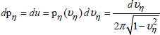

[3.54]

The developments produced in Appendix 4 give the following values to the variances:

[3.55]

It is easy to find from expression [3.50] the average square amplitude of the imaginary component of E_wz:

[3.56]

The following calculation shows that the variance of the real component of E_wz is strictly similar to the previous one:

[3.57]

The simulation of the ideal random field will thus concern the algebraic sum of N plane waves generated according to the process that we have just described. Under these conditions, we can add to the previous field variable, an estimation of its mean value given by the arithmetic mean relationship [3.58]:

[3.58]

We will see in the next section that the properties of the central limit theorem naturally justify the construction of the perfect random field resulting from these N interferences.

3.3.3. Use of the central limit theorem

We immediately deduce from expression [3.58] that the resulting field of the sum of N^th plane waves comes down to the product of the mean estimator and of the size N of the statistical sample thus carried out:

[3.59]

We assume that the polar angle θ, the polarization angle η and the phase angle α are variables randomly distributed with the same probability. Coming back to equation [3.50] shows that the calculation of the moment of the variable found in the sum [3.59] is necessarily zero since this variable is centered:

[3.60]

As a consequence, the interference of an infinite number of plane waves randomly distributed and following the previous criteria, leads to an average null amplitude. If this is a sample of plane waves of finite size N, the resulting amplitude is not strictly null, but is similar to the product of N by the uncertainty of the average estimator expressed in equation [3.59].

We will see in section 3.4.3 that the arithmetic mean estimator is not biased. This currently means that the resulting field amplitude is directly similar to the uncertainty of the average estimation.

Consequently, we can apply to this estimator the Bienaymé-Chebyshev equation recalled below:

[3.61]

This formula expresses the probability of locating the absolute deviation between the mean estimation and the mean value above a given departure h. As justified by the second member of [3.61], the probability will be lower than a value expressed by a quantity inversely proportional to the size N of the sample and dependent on the ratio linking the variance of the field variable to h².

If we link this to section 3.2.1 and more especially to equation [3.4], this property can be extended to the ν variable, i.e.:

[3.62]

In that case, the < ν > estimator is exactly similar to the calculation of the arithmetic mean carried out on a sample of N random ν data, collected in a reverberation chamber.

Whether it is equation [3.61] or [3.62], the mean estimate found in the left member has the sum of N random variables, all following the same probability distribution. We can show that such a process satisfies the Central Limit Theorem (CLT) stating that the probability density attached to the sum of these N variables strives for a normal distribution, when N gets close to infinity. Readers interested in knowing more about the justification of the CLT can refer to [PAP 91] and to section A1.11 of Appendix 1 in this book.

Consequently, we can add to the mean estimate [3.58] the property formulated below:

[3.63]

The σ_<E> parameter found in this expression represents the standard deviation of the mean estimator.

For a large number of N plane waves, we can thus consider that the probability density function of the resulting field gets close to the normal distribution, in which the standard deviation σ_<E> defined above will appear:

[3.64]

The properties of the CLT applied to interferences of plane waves as previously described consequently enable us to compare to the ν variable associated with the ideal random field.

This feature can be extended to the standard deviations, i.e.:

[3.65]

Knowing that the variance of the field variable is connected to the E_w amplitude of the plane waves by equation [3.56], we reach the expression:

[3.66]

Before concluding this section, it is useful to recall that the Bienaymé-Chebyshev equation, as well as the use of the CLT, are dependent on the law of large numbers. Indeed, this is about statistical features meaning that the size N of the samples must be sufficient to carry out the comparison of the plane wave interferences with the ideal random field expected in reverberation chambers. We will see in the next chapter that the physical properties of the cavities necessarily involve the size of the plane wave samples for the simulation of the perfect random fields installed in a reverberation cavity.

3.4. Contribution of the statistical tests

The characterization of the reverberation chambers with the help of statistical tools will be discussed in the next chapter. A few features of these statistical tools will be recalled in this section. On the basis of examples borrowed from the simulation of plane wave interferences, we will see the role given to the size of the sample of data which corresponds to the number N of the random trial.

We will then take a more physical approach to the matter, aiming at comparing the experimental data to the probability density distributions examined at the beginning of this chapter. Section 3.4.3 will be devoted to the estimates of the mean and of the variance formulated by the application of the concepts of maximum likelihood and of bias error. To conclude this section, we will take a more particular look at the statistical Kolmogorov-Smirnov test. Its use for the applications planned in the context of the reverberation chambers seems quite appropriate.

3.4.1. Role given to the size N of the statistical sampling

Let us consider an experiment carried out in a reverberation chamber in which we collect N perfect randomly distributed electric field data. We first assume that the data are expressed in the form of normalized absolute amplitude of the electric field e_r recalled in e_r equation [3.22].

If we have a sufficient sample size N of this data, the law of large numbers will be applied. The uncertainty occurring during the estimate of the mean amplitude of e_r may be calculated from the Bienaymé-Chebyshev formula, stated by equation [3.61] and currently presented in the form of [3.67]:

[3.67]

Let us specify that the estimator < e_r > is related to the complex components of the field and takes the following developed expression:

[3.68]

The “true” mean value determined by the moment of e_r has been previously calculated in [3.29]. We recall the result:

[3.69]

The variance e_r is found on the right of [3.67]. We determine this variance by a calculation, whose main steps will be provided in detail. The variance of e_r comes from the definition introduced in Appendix 1 and reproduced below:

[3.70]

The moment of the square of e_r appears in this formula. It is calculated in [3.30] and can also be found below:

[3.71]

We finally reach the numerical value of 0.429… for the variance.

[3.72]

For the other steps of the calculation, it is interesting to introduce the variance of the mean estimator < e_r > defined as follows:

[3.73]

This relationship confirms an intuitive property, since the probability found in the left of [3.73] can only be lower than the unit. The assumed departure h is necessarily higher than the standard deviation of < e_r >. To illustrate this, it is preferable to convert the gap h using the relative margin ε formed by the ratio of h on the mean value (or expected value) of e_r, i.e.:

[3.74]

If we set the relative margin at 10%, the departure h deduced from [3.74] will be 0.125. For a sample size of N=100, given the variance in equation [3.72], we find that the probability of < e_r > coming out of the [−h +h] gap will be 0.27, i.e. a probability to estimate < e_r > within the gap of 73%. Of course, if we go to a sample of a size ten times larger, these values are 0.027 and a bit more than 97%! These results are explained by the fact that the calculation according to the Bienaymé-Chebyshev formula has a tendency to overestimate the probability of estimating < e_r > out of the uncertainty gap [−h +h]. In fact, we know that the mean estimator obeys the CLT. This means that the probability density can be settled to the normal distribution presented under its normalized form [3.17]. However, the use of this formula requires an additional transformation determined by the entrance of the centered variable z_r in respect of the mean value of e_r and normalized in respect of the standard deviation of < e_r >, i.e.:

[3.75]

Under this form, the application of the CLT allocates to z_r the normal pdf recalled below:

[3.76]

Under these considerations, the probability of finding the absolute value of the z_r variable out side to the [−ζ +ζ] interval is expressed by the integral:

[3.77]

So that this equation is in accordance with the previous calculation, we must establish the link between the h and ζ quantities, which are easily deduced from equations [3.73] and [3.75], i.e.:

[3.78]

During the previous numerical example, h took the value of 0.125. Thus, for a sample size of 100, the gap ζ calculated from [3.78] is worth 1.90.

Integral [3.77] does not have an analytical solution. Thus, the calculation will be carried out by consulting Table A1.2 in Appendix 1 or with the help of specific software. The table gives a number close to 0.05, i.e. a 95% probability of entering the gap, but a 73% probability from the direct application of the Bienaymé-Chebyshev equation.

The test obtained by the application of the CLT thus enters the gap more easily, and this estimation uncertainty is generally called by the statisticians the confidence interval.

This example has also shown the important role played by the size N of the statistical sample. The latter however has a different meaning, depending on whether we aim at the analysis of measurement results or the simulation of perfect random field by the interference of plane waves.

During a simulation, the choice of the size N must be guided by the physical properties of the reverberation chamber. We have shown that the construction of one mode requires the interference of eight plane waves. Furthermore, the contribution of the quality factor of the cavity is added to this, which imposes the bandwidth Δf₀ as soon as the cavity is excited at the frequency f₀. This narrow band will thus select N_w other modes that we can approximate by forming the product of Δf₀ with the density functions of the modes D(f₀) taken from the Weyl formula, i.e.:

[3.79]

We will see in section 4.2.3 of Chapter 4 that the advantage of this simulation is to calculate the power collected by the transmission lines of the printed circuits contained in most electronic equipment submitted to electromagnetic tests.

3.4.2. Assessment of the experimental data to the probability distributions

An important stage in the analysis of the physical behavior of the reverberation chambers consists of checking if the data recorded during the collection of powers captured by an antenna or of field values supplied by a probe follow a known probability distribution. The most elementary tests consist of evaluating a chamber compared to the hypothesis of the ideal random field distribution: i.e. whether we can compare it to an exponential function for power data or to a Rayleigh’s distribution for absolute amplitude of field data. These data can come from measurements carried out in the chamber or from numerical simulations carried out with the help of full-wave Maxwell solvers. Several methods are commonly used to perform this type of calculation, such as the finite element method, the finite difference time domain method or the method of moments.

3.4.2.1. Power data collected on a receiver

Let us consider the normalized power p_r defined in section 3.2.3 and recalled below:

[3.80]

It was shown in section 3.2.4 that under the hypothesis of the ideal random field, the p_r random variable is attached to the exponential probability density function, i.e.:

[3.81]

The assessment consists of drawing function [3.81] and of comparing it to a histogram built on the basis of N data of normalized power collected during an experiment. As shown with more detail in section 4.4 of Chapter 4, these data can come from sampling carried out during a revolution of the mode stirrer.

However, practice shows that it is generally inconvenient to extract the curve from the histogram of the probability density function, thanks to several erratic fluctuations that are due to the necessarily limited size of the statistical sample. For this reason, we will adopt the histogram built on the integral of the cdf (cumulative distribution function) defined in Appendix 1.

The cdf designated by the F₂(p₀) symbol is recalled in equation [3.82]. This function sets the probability of finding the p_r variable, equal to or lower than a p₀ threshold continuously evolving between the null minimum value and the p_{r maxi} maximum value set by the upper limit of the sample:

[3.82]

With the resolution of the integral being immediate, we reach the analytical function [3.83]:

[3.83]

The layout deduced from this formula will thus constitute the reference curve adopted for the comparison of the histogram. The histogram comes from the batch of N pieces of data contained in the (P_r)^t vector reproduced below:

[3.84]

The components of these vectors are spread by increasing values in accordance with the rule established in equation [3.85]:

[3.85]

The S_N(p₀) histogram deduced from this classification will thus allocate to the piece of data p_r, the probability calculated by the ratio linking the row k to the size of the sample N, i.e.:

[3.86]

If we find two identical components of the (P_r)^t vector, one of the values will be slightly modified to come out of the singularity. The probability of such an event is generally very low.

The graph in Figure 3.2 reproduces the histogram of the data of powers collected on a receiving antenna during a revolution of the mode stirrer. The size of the sample is close to 100. Some data are probably correlated, but this does not alter in any way the reproduction of the histogram. The horizontal axis of the graph carries the normalized values p_r calculated on the basis of the physical data of power p (in Watts) gathered during the experiment. Relationship [3.80] recalled above, shows that the determination of p_r requires the evaluation of the p_mv mean value of the power rigorously defined by the moment of the p variable.

The latter being a priori unknown, p_r can only be calculated by forming the ratio of p and of the mean estimate carried out on the concerned statistical sample, i.e.:

[3.87]

The reference curve designated by the continuous line in Figure 3.2 corresponds to the cdf F₂(p₀) deduced from analytical function [3.83], where the reduced variable p₀ is expressed under the convention:

[3.88]

The comparison of the histogram and of the reference layout shows that there is no rigorous agreement. These deviations are thus the sign of a shift compared to the expected cdf. In this case, the cdf results from the exponential probability density function.

We will see in the last part of this section that the statistical tests evaluate the tuning probability of the S_N (p₀) histogram brought back to the reference distribution function F₂(p₀).

3.4.2.2. Voltage data collected on an electric field probe

Most of the electric field probes used in the measurement chains give voltages proportional to the amplitude of the electric field vector , polarized in parallel with the sensitive elements of the probe. Figure 3.3 shows the example of a symmetric electric dipole directed according to the oz axis of the oxyz coordinate system.

The probe produces the V_c voltage proportional to the absolute amplitude of the electric field directed according to oz, i.e.:

[3.89]

The K₀ coefficient is thus a conversion factor of physical scale. In expression [3.22] established in section 3.2.3, the normalized variable e_r of the absolute amplitude of the electric field was introduced. We will recall below the definition applied to the probe in Figure 3.3:

[3.90]

There is in this formula standard deviation of the ν variable attached to the real and imaginary components of the complex E_z variables, i.e.:

[3.91]

According to the hypothesis of the ideal random field distribution, it was shown in section 3.2.5 that the pdf attached to e_r was Rayleigh’s distribution recalled below:

[3.92]

If we introduce the normalized voltage variable under the v_r symbol, which is more precisely defined by equation [3.93]:

[3.93]

we realize that v_r is immediately related to e_r. We can thus attach to the normalized voltage the Rayleigh’s pdf found in [3.92].

As previously practiced for the power, we can attach to the normalized voltage the pdf F_R(v₀) resulting from the integral of the pdf, i.e.:

[3.94]

The transfer in normalized variables will require the determination of the standard deviation of V_c. This parameter will be taken from an estimate carried out according to the features exposed in the next section.

3.4.3. Estimate of the variances and means

The question of the estimate of the variances and means is closely linked to the research of criteria of the likelihood maximum and of the bias factor. We will limit the demonstration to the case of normal distribution. This theoretical approach could however be easily extended to other probability distributions.

Let us consider a continuous random x variable governed by the complete normal distribution recalled below:

[3.95]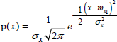

There is in this formula the moment and the variance of x taking as definitions:

[3.96]

[3.97]

We will first carry out the formulation of the estimators.

3.4.3.1. Search for the estimator giving the likelihood maximum

The normal pdf [3.95] can be expressed in the form of a P(a,b,x) function of the x variable, where a and b are parameters respectively designating the first moment and the standard deviation of the random x variable:

[3.98]

Let us consider a set X containing N variables x all assumed to be independent and stationary:

[3.99]

The P_N probability of carrying out the set X is thus determined by the product of N functions [3.98], i.e.:

[3.100]

Under these hypotheses, research on the estimators of the a and b parameters giving the most significant likelihood must necessarily converge on a maximal P_N probability.

This condition can be easily formulated by setting that the partial derivatives of P_N with respect to the a and b parameters will be null, i.e.:

[3.101]

Knowing that the calculation will be simplified when going through the logarithmic derivatives, equation [3.101] becomes:

[3.102]

The calculation of the derivatives mentioned above leads to equations [3.103] and [3.104]:

[3.103]

[3.104]

We take from the first equation the estimator of the mean of x presented with the appropriate notation < x >:

[3.105]

We take from the second equation the variance estimator, i.e.:

[3.106]

The demonstration leads to formulas in good accordance with the intuitive choices.

3.4.3.2. Evaluation of the bias error

Without bias errors, the average of an infinite quantity of estimators [3.105] and [3.106] must necessarily converge on mean and variance values, as given by the moments definition. This means that calculation of the expected value applied to the second members of the previous equations must be identified with the moment and with the variance of the x variable.

For the mean estimator, the calculation gives the expected agreement:

[3.107]

We can thus conclude that the mean estimator deduced from [3.105] is not affected by the bias error.

If we carry out a similar calculation for the variance after using the expression located on the right of [3.106], we reach the following result:

[3.108]

The right side of this expression proves that the variance estimator is biased by a coefficient determined by the (N−1)/N ratio. Nevertheless, for an infinite size of the sample X, calculation [3.108] converges on the true value of the variance.

To eliminate the bias error, we just need to invert relationship [3.108] from which we find the unbiased variance estimator, i.e.:

[3.109]

Let us specify that for relatively vast X sets, formulas [3.108] and [3.109] of the variance estimator lead to very close numerical values.

3.4.4. Kolmogorov—Smirnov test

3.4.4.1. Introduction to the KS test approach

Let us consider a set of N random data. Its histogram of amplitude distribution will be compared to a known theoretical distribution function. If this is about the power collected on a receiving antenna installed in a reverberation chamber, the N data makes up the S_N(p₀) histogram built in [3.86], whereas the theoretical cumulative distribution function F₂(p₀) is taken from the analytical formula [3.83] [LEM 08, MAS 51, PAP 91].

To evaluate the probability of S_N(p₀) belonging to the F₂(p₀) layout, we can practice the χ² test, which is profusely described in most of the books discussing statistics. However, we know that the optimal use of this test can only be carried out on samples with generally lower size. For higher populations, this test is only available when we make groupings of data which cause inaccuracies in the final use of the result.

Knowing that the populations collected during measurements in a reverberation chamber will have a size much higher than 10, the experiment shows that it was better to adopt the Kolmogorov—Smirnov test. We propose recalling the principle of this test according to the works published by F.J. Massey [MAS 51].

The KS test can be applied to various probability distributions. The variable will be designated by the x symbol, the reference cdf by F(x) and the experimental histogram by S_N(x).

We adopt a statistical distance made up of the absolute value of the maximum Δ_m deviation collected between the experimental histogram and the theoretical distribution function of reference F(x), i.e.:

[3.110]

To confirm the agreement with the expected probability distribution, the Δ_m gauge is compared to a Δ_c critical value found within a table of numerical data. This critical value is governed by two parameters: the level of significance α so called risk threshold and the sample size N.

Table 3.1 replicates the table of the critical values published in the work of Massey [MAS 51]. The statistical parameters have the risk threshold evolving from the minimum value 0.01 to the maximum value 0.20 under a step of 0.05 and for sample sizes ranging between 1 and 35.

Thus, by setting the risk threshold at 0.05 and for a sample size of 15, the critical value Δ_c is worth 0.338. This means that if we have a Δ_m distance lower than 0.338, the experimental histogram has the 1−α probability of belonging to the selected theoretical cdf, i.e. currently a confidence probability of 95%. In the opposite case, i.e. Δ_m is higher than 0.338, the test is rejected.

For the sample sizes higher than 35, Δ_c can be approximated by an analytical expression. For example, for a risk threshold of 0.05 and a sample of size 50, the use of the formula located at the bottom of Massey’s table recommends the critical value 0.192 calculated below:

[3.111]

This example shows what intuition was predicting: that any growth of the sample size comes down to a reduction of the critical value and consecutively to a more stringent test.

3.4.4.2. Construction of Massey’s table

Before carrying on with the investigation concerning the use of the KS test, it is essential to specify some details on the method adopted to build Massey’s table. The author has chosen the normal distribution as a reference. We will recall here its probability density function for an centered variable x:

[3.112]

In this function, the standard deviation σ_x is the only essential parameter for the formulation of the probability distribution. In the presence of a sample of N experimental data, this parameter is unknown. σ_x will thus be estimated by the processes examined in the previous section. To summarize, this means that each sample corresponds to a reference distribution that is its own. To free ourselves from this practical difficulty, Massey’s table has been created by using an invariant standard deviation or by taking, as a base, normalized variables θ without physical dimension. This amounts to strictly the same as the first method.

The normal distribution then takes as an expression function [3.17] which was introduced in section 3.2.3 and transcribed under the current notations:

[3.113]

We can easily deduce from this expression the cdf designated by the F_n(θ₀) symbol, where the n index means that we aim at the normal cdf:

[3.114]

This integral containing the Gaussian function does not have an analytical solution. Thus, we use a numerical computation of [3.114] as found in Table A1.1 in Appendix 1.

The calculations of the critical values have thus been practiced on the basis of collections of samples of growing size N, coming from Monte Carlo trials. In order to meet the criteria required by the large numbers law, the experiments should have concerned collections greater than 1,000 batches of N data. This guarantee thus allows us to produce a reliable estimate of the risk factor α.

3.4.4.3. Simulation of the KS test

Simulation of the KS test can be carried out for the generation of N data by the Monte Carlo trials. Let generate such a sample of the random normalized variable v_r, whose probability distribution is given by the exponential cdf from equation [3.83]. With the current notations, this equation is expressed:

[3.115]

We know that F₂(v_r) represents a probability whose numerical value u is naturally in the interval [0 1].

With this condition, equation [3.115] will be inverted, in order to make available one trial of the x variable:

[3.116]

This equation leads to the generation of a sample of N variables of x trials from the N values of u, produced by a set of numbers with uniform random distribution.

The layout of the S_N(X₀) histogram, displayed by the empty circles in Figure 3.4, has been made in accordance with the simple computation given in equation [3.86].

Concerning the theoretical reference curve, the calculation comes from the cdf of the exponential distribution presented under the following form:

[3.117]

The full circles in Figure 3.4 correspond to the product of this calculation. The curve linking the points is a straight-line interpolation. In formula [3.117], the < x > estimator of the mean value of the x variable is found:

[3.118]

The maximum distance recorded between the histogram and the reference, which has been defined according to the prescriptions of relationship [3.110], is currently located at Δ_m = 0.201.

We practice 10,000 trials with random data which are renewed each time. The obtained result shows that 2% of the experiments overcome the standard deviation of 0.201. Massey’s table indicates, on the line N = 30, that a critical value of 0.200 should give a rejection rate located between 10% and 15%.

The experiment is thus more tolerant than the indication of the table. The origin of this behavior probably lies in the construction of Massey’s table, based on the normal distribution. We will see in Chapter 8 that the strictness of the test can be increased by the adoption of Lilliefors’ table, which is established using the exponential probability distribution. However, the international standard relative to the tests performed in reverberation chambers recommend for now the Massey tables. This choice thus justifies the maintaining of this statistical reference.

3.5. Balance of power in a reverberation chamber

This section summarizes the main antenna properties, their theoretical bases will be detailed in Chapter 6. Regarding the hypothesis of a continuous sine wave excitation, antenna parameters such as efficiency, directivity and gain will be recalled. This introduction will facilitate the reading of section 3.5.2 devoted to the behavior of a receiving antenna installed in a reverberation chamber. It will then be shown that the power collected at the output of an antenna illuminated by an ideal random field is impervious to the directivity. These theoretical notions will help to make the link with the power radiated by an object immersed in a reverberation chamber and to define measurement procedures.

3.5.1. Review of the main features of antennas

The electromagnetic sources essential for the calibration of the reverberation chambers or for radiated emission tests will be made up of antennas or devices, whose main electromagnetic properties are summarized in this section.

Figure 3.5 shows a transmission antenna attached to a spherical coordinate system orθφi.

3.5.1.1. Antenna efficiency

The P_i parameter represents the power injected by the RF generator, P_ρ is the power reflected by the antenna and P_tr the power transmitted and radiated outside the AA’ plane constituting the physical boundary of the antenna and currently open in free space.

If the propagation of the spherical wave is carried out in a non-lossy media and without any obstacle, P_tr is related to the flux of the Poynting vector, calculated through the sphere of radius r centered on the origin of the graph, i.e.:

[3.119]

The and vectors in this integral are thus attached to the wave radiated at any point of the space. The star on the symbols means that this is the conjugate complex amplitude.

Generally, the radiated power is a complex number, whose real component is preserved with the distance r. The electric and magnetic field vectors follow the scattering law, inversely proportional to the r distance. However, the imaginary component of the power is vanishing. Concretely, this means that the fields attached to the vanishing wave take a weak amplitude as soon as the r distance overcomes the wavelength.

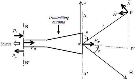
An essential parameter for the physical understanding of the measurements practiced in reverberation chambers is the antenna efficiency. In the BB’ input plane where the source is located, the P_ta transmitted power will be represented by the difference between the P_i injected power and the P_ρ, i.e.:

[3.120]

For various physical reasons, mainly due to thermal losses in the antenna, the P_tr power radiated outside the AA’ plane will be lower than the P_ta transmitted power in the BB’ plane. This property is expressed in relationship [3.121] where the η coefficient, so-called antenna efficiency, represents the efficiency of the antenna:

[3.121]

If these antennas are designed to carry out electromagnetic immunity tests, the η efficiency is close to one unit. For biconical or log periodical antennas, this factor is located close to 0.75. In other cases, it can also be lower than one unit. Efficiencies very much lower than unity may be found during the measurement of the radiation leakages produced by devices such as cables or shielded connectors. The measurement procedures require that the terminations of cables or connectors are connected at one end to a RF generator and with the other end matched to their characteristic impedance. This configuration typically represents a device whose η antenna efficiency is much lower than one unit. This property is easily explained since the leaky radiated power P_tr through the shields only represents a tiny part of the transmitted power P_ta in the terminal load.

3.5.1.2. Directivity of an antenna

The directivity of the antenna or of the device is determined by the radiation pattern often displayed with curves in spherical coordinates. Depending on the case, the angular coordinate illustrates the elevation angle θ and the azimuth angle φ. The layout is the locus of the radial distances, on which the field amplitude remains invariant as a function of the θ variable or of the φ variable. The directivity is generally defined for the far-field. It is normalized compared to the peak field magnitude collected on the ranges covered by θ and φ. In some cases, the directivity can be expressed in terms of a normalized analytical function without physical dimension versus the θ and φ variables, which can be merged under the solid angle Ω.

3.5.1.3. Gain of an antenna

The gain of an antenna is associated with the peak field amplitude collected on the radiation pattern, but with respect to a reference antenna, whose radiated power would be strictly similar to the one produced by the antenna involved. The gain is usually expressed on a dB scale. The physical reference is generally constituted by an antenna with a perfect isotropic radiation or sometimes by an electric dipole.

There is a more detailed description recalling the physical basis of the functioning of antennas in section 6.2 of Chapter 6.

3.5.2. Receiving antenna immersed in an ideal random field

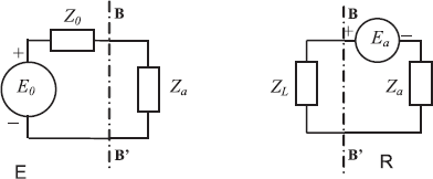
In the BB’ input plane of the transmitting antenna illustrated in Figure 3.5, we can add the equivalent circuit shown on the left in Figure 3.6. The E₀ and Z₀ parameters respectively designate the emf and the internal impedance of the HF source connected on the antenna. The Z_a antenna located on the right of the BB’ plane amounts to the input impedance of the antenna. For a properly constituted antenna, Z_a is similar to a resistance, in which the energy losses would be composed of the thermal power lost in the antenna and the power radiated under the electromagnetic form. Let us specify that the optimal energy transfer assumes that the inner impedance of the Z₀ source is strictly equal to the conjugate input impedance of the antenna. When these conditions of adaptation are met, we must cancel out the reflected power P_ρ by connecting a transmission line between the output of the generator and the input of the antenna whose characteristic impedance is as close as possible to Z_a, if it is real.

Under the configuration of the diagram on the right in Figure 3.6, the receiving antenna is connected to the load impedance Z_L. There are, in the right part of the BB’ plane, the E_a emf induced by the surrounding electromagnetic field and the internal inner impedance of the receiving antenna. By application of the reciprocity principle, the inner impedance of the receiving antenna is the input impedance of the transmitting antenna. This comparison is however subordinated to the conditions of linear behavior [GOE 03].

The theoretical problem set by the immersion of a receiving antenna in a reverberation chamber thus consists of calculating the power collected by the antenna subjected to an ideal random field. The hypothesis of an perfectly matched antenna is added to this prior condition, i.e. connected on a load impedance that is strictly similar to its inner impedance. To do this calculation, we will adopt the work of D.A. Hill published in 1998 [HIL 98].

In this original approach, the field surrounding the antenna is made up of the interference of the ideal random plane waves. We will only mention the main stages of the computation, based on the use of the plane wave spectra introduced in section 2.3.8.

Let us consider the plane wave spectrum. We extend the definition of formula [2.88] to the case of the electric field vector as a function of three x, y, z variables of a Cartesian graph:

[3.122]

This expression can be inverted to the advantage of equation [3.123]:

[3.123]

This relationship means that any linear transformation applied to the electric field vector (x,y,z) will also be applied to the plane wave spectrum (k_x,k_y,k_z). Let us specify that the D⁻¹ symbol at the bottom of the integral corresponds to the space of the wave numbers, which corresponds to the space D initially found in [3.122]. In section 3.3.1, it was shown that a reverberation cavity excited on its eigenmodes is equivalent to describe a spherical surface with the extremity of the wave number vector . Consequently, the transformation of equation [3.123] in the coordinate system in Figure 3.5 gives the double integral shown below:

[3.124]

In this equation, we go to the Cartesian projections of the vector, in return for the use of the transformation relations set out in [3.38]. The θ' and φ’ integration variables must be in the vector, whereas the θ and φ space variables remain in the expression of the vector.

For a given excitation frequency of the cavity, the absolute value of the vector is an invariant that we can include in the spectral density function. Moreover, if we introduce the solid angle Ω, integral [3.124] takes the more simple form [3.125]:

[3.125]

The (Ω) spectral function will be used in the following. This function includes the 1/4π factor found in the previous relations.

Under the assumption of an ideal random field, the values of the functions (r,θ,ϕ) and (Ω) behave like centered random variables; this is in accordance with the hypotheses stated in section 3.2.1. We know that the mean amplitude value of these variables according to the moment calculation of the expected value leads to zero:

[3.126]

However, the developments detailed by Hill show that the moment of the square of the field amplitude leads to integral [3.127] which may be solved immediately.

[3.127]

In this equation, the C_E parameter represents a physical scale coefficient with unit in (V/m)². In the context of relationship [3.127], the result of the calculation is thus strictly similar to the square of the constituents of the uniform amplitude E_w of the plane waves entering in the spectrum.

[3.128]

Then, carrying out the determination of the moment of the electromagnetic energy stored in the reverberation cavity, Hill manages to relate the amplitude of the plane wave spectrum to several parameters among which we find: P_tr the power radiated by the transmitting antenna, ω₀ the excitation angular frequency, Q the quality factor of the reverberation cavity, V the volume of the chamber, as well as ε₀ the absolute electric permittivity:

[3.129]

Knowledge of E_w finally enables us to undertake the calculation of the P_cr power collected on the Z_L load, itself connected on the receiving antenna. This stage is to be linked with the configuration of the diagram in Figure 3.6 and for the perfectly matched antenna. The first hypothesis means that the inner impedance of the Z_a antenna is strictly equal to the R_r radiation resistance and that the load impedance is also similar to R_r. In other words, the η antenna factor of the receiving antenna is strictly one. Under these conditions, Hill reaches the calculation of the moment of P_cr Its value is then expressed in terms of the integral [3.130]:

[3.130]

This equation contains the impedance of the plane wave Z_w, the wavelength of the exciting field λ, as well as D(Ω) the directivity of the receiving antenna. Knowing that we practice the integral computation on the full domain covered by the solid angle Ω, this integral takes the value 4π. Consequently, the mean value of the amplitude of the power collected on the perfect matched receiving antenna without losses is then expressed by:

[3.131]

The obtained formula is thus very consistent with respect to the physical features of the receiving antenna induced under a perfect random field. The ½ factor takes into account the balanced probability of the polarization of the plane wave spectrum. Let us imagine that the antenna is only sensitive to the polarized electric field following the oz direction merged with the polar axis of Figure 3.5. The antenna will thus be sensitive to any plane wave projecting the electric field E_z in the BB’ plane, but it will not be affected by the waves projecting the magnetic field H_z. Consequently, only half of the waves randomly polarized in the spectrum can excite the receiving antenna. The second ratio found in [3.131] expresses the power density of the plane wave spectrum, whereas the third ratio represents a surface that determines the mean effective area of the perfectly matched and lossless receiving antenna, [ELL 81]. When the antenna is partially mismatched and subject to thermal losses, we substitute in [3.131] the mean effective area _e. This parameter includes the ½ factor accounting for the balanced polarization of the waves, a mismatch factor m and then the antenna efficiency η resulting from a calculation or a measurement:

[3.132]

We finally reach the final form [3.133] of the mean power collected by the receiving antenna:

[3.133]

3.5.3. Measurement of the power radiated by a device in a reverberation chamber

The power radiated by a device immersed in a reverberation chamber can be evaluated thanks to the determination of the power collected from a receiving antenna. By combining relations [3.129] and [3.133], we obtain a single expression where we can deduce the radiated power P_tr from the device, i.e.:

[3.134]

However, measurements in that case consist in collecting a finite sample of power data in the reverberation chamber Therefore, this relationship must be immediately transformed into an estimate of the mean amplitude, using the dedicated notations:

[3.135]

This formula shows that the determination of the radiated power is strongly dependent on knowledge of several physical parameters of the reverberation cavity, such as the quality factor Q and the volume V. Other parameters are also concerned. They relate to the receiving antenna and are gathered in the average effective area _e . Uncertainties are assigned to all these data. These are more or less able to affect the reproducibility of the measurements. To decrease its impact, we carry out a calibration with the help of a transmitting antenna with a known antenna efficiency η_e. Knowing that we inject into this antenna the power P_i, the determination of the reflection coefficient ρ_e observed in the BB’ plane, as is illustrated in Figure 3.5, immediately gives access to the transmitted power by using equation [3.136]:

[3.136]

Determination of P_tr0 the power radiated by this calibration antenna thus involves the η_e factor in expression [3.137]:

[3.137]

The transmission of the P_tr0 so-called reference power will correspond to the power collected on the receiving antenna, expressed in terms of the < P_cr0 > estimator. Relationship [3.135] established above will thus form the link between transmitting and receiving powers, within the reverberation chamber. Converted in equation [3.138], this formula gathers into the A coefficient the physical parameters of the chamber and of the receiving antenna. It is no longer essential to know these parameters:

[3.138]

Indeed, by following the measurements procedure, we replace the transmitting antenna with the device radiating the unknown power P_trX. Under this new configuration, the receiving antenna collects the power < P_crX > that we relate to P_trX with an expression similar to [3.138]. The new formula [3.139], mentions the A’ coefficient which is a priori different from A:

[3.139]

Let us not forget that the substitution of the device for the reference antenna more or less alters the value of the quality factor, as well as the volume of the chamber and consecutively the coefficient A.

If we take care to maintain the device and the transmitting antenna in the chamber for all phases of the experiment, the energy losses will be almost unchanged. The impact on the coefficient A will thus be negligible and we will be able to find < P_trX > by using the simple equation formulated below:

[3.140]

We must specify that the calibration power P_tr0 appearing in [3.140] is not necessarily an estimated variable, since it involves quantities that are assumed to be invariant, i.e. the P_i injected power and the reflection coefficient of the antenna ρ_e found in expression [3.137].

However, we must consider that this reflection coefficient can somewhat change with the angular position of the mode stirrer. The cause of this physical mechanism is the backscattered power in the transmitting antenna. This backscattered power depends on the conditions involved by the modal excitation of the room. For this reason, it seems more accurate to make the calibration with the estimated value of < ρ_e >.

3.6. Discussion

3.6.1. On the hypothesis of the ideal random field

The perfect reverberation chamber is mainly based on the postulate that the field data collected in the chamber gets away from any deterministic process. Indeed, this assumes that the field, produced by a transmitting antenna installed in the chamber, is entirely converted in the form of standing waves distributed according to a stochastic process. Under these conditions, the data collected would be statistically independent. In fact, these hypotheses are partially questionable!

If the first is indeed verified in acoustics where we have compact sources transmitting little scattered beams, the transmission of the Hertzian waves is often carried out with limited directivity, whose consequences are damaging for the production of ideal random fields.

Let us take two examples: in a first experiment, we carry out the emission inside the room with the help of a horn antenna pointed at the opposite side to the measurement location of the field. In a second experiment, the antenna used gives an almost isotropic radiation. It is certain that in the first case, the resulting field intercepted at the measurement location will be richly composed of standing waves formed by the interference of the successively reflected beams coming from the horn antenna. The conditions are thus highly favorable for the installation of an ideal statistical distribution of the field. Conversely, the direct radiation from the isotropic antenna used in the second experiment will more or less influence the resulting field at the measurement location. Two scenarios may occur, depending on the value of the quality factor of the chamber.

In the case of a very high quality factor, the direct field produced by the antenna will be masked by the very strong amplitude of the standing waves due to the resonances. However, we know that high quality factors reduce dramatically the modal bandwidth. So does the number of standing waves involved in the interference process leading to the random behavior of the field. This scenario thus goes against a perfect random field.

Fall of the quality factor will favor the contribution of the direct field, whose amplitude can then overcome the resulting field due to the standing wave interferences, though it is much more numerous than previously. The over-significant contribution of the direct field thus has the effect of moving the field distribution away from perfect random process

The expected behavior of the field should thus satisfy a compromise between two previously illustrated conditions. As is very well justified by the previous works of C.L. Holloway, the field distribution in a reverberation chamber, which is expressed in terms of the probability density function of an absolute amplitude, should be located between the ideal random field represented by Rayleigh’s distribution and Rice’s distribution, where a significant contribution of the direct couplings is involved [COR 00, HOL 06].

The second postulate requiring statistically independent data is more subjective, because the fields results from standing waves. Their amplitudes are locally correlated in the space. This matter will be covered in more detail in Chapter 4..

3.6.2. On the simulation of the disordered field by plane waves trials

We showed in section 3.3.3 and after the application of the central limit theorem, that N plane waves of uniform amplitude having an incidence angle, polarization angle and a phase drawn at random, produced an ideal random resulting field. It was also proven with the help of basic statistical theories that the standard deviation of the resulting field evolves inversely from the square root of the sample size N involved.

The simulation nevertheless relies on the application of the ergodism principle, where we replaced the physical variations of the random amplitude of the waves with the random variations of their incidence angle. It is possible that under the hypothesis of large numbers, the two methods converge.

In practice, the simulation will require the assistance of the trials and tests. The tests will correspond to the angular positions of the mode stirrer giving independent data. The trials consist of restituting the ideal random field renewed on each test. If one test has N trials, a revolution of the mode stirrer generates N_B tests. The criterion chosen for determining N comes from the physical properties of the plane wave spectra, which are presented in section 2.3.8, and from the N₀ amount of the sine functions entering in the Δf₀ selection band. Let us recall that the modal bandwidth, also called the modal selection band, is dependent on the quality factor of the chamber excited under the emission frequency f₀. Knowing that each function is similar to eight plane waves, each test should thus have 8N₀ trials. Concerning the criterion chosen for the number of tests, N_B will be set by the shape of the auto correlation function of the mode stirrer as is described in section 4.4.2 of Chapter 4.

Simulations by plane waves trials designed for the calculation of the power induced on a line parallel to a ground plane similar to the device, in Figure 4.1, section 4.2.3 of Chapter 4, have been successfully carried out by L. Musso [MUS 03]. The curves recorded from the simulations corresponded to measurements showing that the experimental and theoretical margins were quite in accordance with one another.

However, respecting the random trials assumes the statistical independence of the incidence, polarization and phase angles. This hypothesis can be questionable as soon as the amount of the modes entering Δf₀ dramatically grows as the excitation frequency increases. We can thus fear that adjacent modes may become significantly correlated in polarization and phase amplitude. These imperfections probably have an impact on the calculations carried out for a chamber that is hyper-sized compared to the wavelength; i.e. during experiments practiced above 10 GHz and for chambers of “volume” at least higher than 10 m³ [COZ 09].

3.7. Bibliography

[BAS 67] BASS J., Eléments de calcul des probabilités, théorique et appliqué, Masson, Paris, 1967.

[COR 00] CORONA P., FERRARA G., MIGLIACCIO M., “Reverberating chamber electromagnetic field in presence of an unstirred component”, IEEE Transactions on Electromagnetic Compatibility, vol. 42, no. 2, p. 111–115, May 2000.

[COZ 09] COZZA A., “Statistics of the performance of time reversal in a Lossy reverberating medium”, Physical Review, E80, 056604, November 2009.

[ELL 81] ELLIOT R.S., Antenna Theory and Design, IEEE Press, New York, 1981.

[GOE 03] GOEDBLOED J.J., “Reciprocity and EMC measurements”, International Symposium on Electromagnetic Compatibility, Tutorial lecture, Proceeding, p. 1–12, Zurich, February 2003.

[HIL 98] HILL D.A., “Plane wave integral representation of fields in reverberation chambers”, IEEE Transactions on Electromagnetic Compatibility, vol. 40, no. 3, p. 209–217, August 1998.

[HIL 08] HILL D.A., “Probability density function of power received in a reverberation chamber”, IEEE Transactions on Electromagnetic Compatibility, vol. 50, no. 4, p. 1019–1019, November 2008.

[HOL 06] HOLLOWAY C.L., HILL D.A., LADBURY J.M., WILSON P.F., KOEPKE G., CODER J., “On the use of reverberation chambers to simulate a Rician radio environment for the testing of wireless devices”, IEEE Transactions on Antennas and Propagation, vol. 54, no. 11, p. 3167–3177, September 2006.

[KOS 91] KOSTAS J.G., BOVERIE B., “Statistical model for a mode stirred chamber”, IEEE Transactions on Electromagnetic Compatibility, vol. 33, no. 4, p. 366–370, November 1991.

[LAD 99] LADBURY J.M., “Monte Carlo simulation of reverberation chambers”, Proceedings of the 18^th Digital Avionic Systems Conference, vol. 2, p. 10.C-1-1-10.C-1-8, October 1999.

[LEM 08] LEMOINE C., Contribution à l’analyse statistique des mesures en chambre réverbérante à brassage de modes, Thesis, INSA of Rennes, 2008.

[MAS 51] MASSEY F.J., “The Kolmogorov-Smirnov test for goodness of fit”, Journal of the American Statistical Association, vol. 46, p. 68–78, 1951.

[MUS 03] MUSSO L., Assessment of reverberation chamber testing for automotive applications, PhD Thesis, Politecnico di Torino, Lille 1 University, 2003.

[PAP 91] PAPOULIS A., Probability, Random Variables, and Stochastic Process, McGraw-Hill, New York, 1991.

[SER 09] SERRA R., CANAVERO F., “Reconciling statistical models with practical experience of reverberation chambers”, Electronic Letters 26, vol. 45, no. 5, February 2009.