
12
Power Flow in Damped Structures
12.1 Introduction
Extensive efforts have been exerted recently to quantify the power flow and energy transmission paths in vibrating structures. Such a quantification process is essential to the design of appropriate passive/active vibration control systems for these structures. In these control systems, the emphasis is placed on altering/confining the transmission paths to uncritical zones of the vibrating structures or minimizing the power flow across paths encircling the disturbance zones.
Several approaches have been considered for identifying the power flow, which is also known as structural or mechanical intensity, in vibrating structures. Distinct among these methods are: the Statistical Energy Analysis (SEA) method (Lyons 1975), the finite element method (FEM) (Garvic and Pavic 1993; Pavic 1987, 1990, 2005; Alfredsson 1997; Alfredsson et al. 1996), the FEM with heat conduction analogy (Nefske and Sung 1987; Wohlever and Bernhard 1992; Bouthier and Bernhard 1995), and a wide variety of experimental methods (Noiseux 1970; Pavic 1976; Williams et al. 1985; Williams 1991; Linjama and Lahti 1992; Gibbs et al. 1993; Halkyard and Mace 1995). Comprehensive and critical reviews of structural power flow are given by Mandal et al. (2003) and Mandal and Biswas (2005).
It is important here to note that the SEA is particularly suitable for computation of the average spatial power flow in the high frequency domain. The classical FEM is, however, more suitable for low‐frequency predictions of the spatial distribution of the power flow. For medium frequencies, the FEM with heat conduction analogy has been shown to accurately predict the power flow in beams, membranes, and plates.
In here, our focus is devoted to the use of the classical FEM as the basic tool for computing the power flow in structures. The prediction accuracy of the FEM is checked against the predictions of classical distributed‐parameters methods (Wohlever and Bernhard 1992).
Also, particular attention is given here to the control of the power flow in damped structures.
12.2 Vibrational Power
12.2.1 Basic Definitions
Consider the following vibrating structure:
where [M], [C], and [K] are the mass, damping, and stiffness matrices. Also, {X} and {F} are the vectors of nodal deflections and external loads.
For sinusoidal excitations, the mobility YF of this structure is given by:
where GF is the “conductance” and BF the “susceptance” matrices.
The complex vibrating power, SP, supplied by the external loads {F} is given by:
where {.}* is the Hermitian transpose of {.}, that is, the transpose and complex conjugate of {.}.
From Eq. (12.2), one can write ![]() as follows:
as follows:
Substituting Eq. (12.4) into Eq. (12.3) yields:
and
12.2.2 Relationship to System Energies
Equation (12.2) can be rewritten as:
Hence,
But, as the [K], [C], and [M] matrices are symmetric and real, then:
From Eqs. (12.3) and (12.8), the power S can be determined from:

and
where
From Eq. (12.10), the active power, PF, depends on the damping matrix [C] so it defines the power dissipated in the structures. The reactive power, QF, is proportional to the difference between the potential and kinetic energy.
12.2.3 Basic Characteristics of the Power Flow
The reactive power, QF, vanishes at natural system frequencies
Proof
Eq. (12.10) can be rewritten as:

Hence, QF = 0 implies that:or,
that is,
which means that ω2 is an eigenvalue of [M]−1[K] and {X} is the corresponding eigenvector.
Hence, the total power flow at resonance is reduced to the active power flow component PF, that is,
Solution
The system response x is given by:

where ω, ωn, and ζ are the excitation frequency, the natural frequency ![]() and the damping ratio =c/(2m)ωn.
and the damping ratio =c/(2m)ωn.
Then,

or,

with

which gives:

and

Figure 12.1 displays the active and reactive powers as function of the frequency ratio Ω for ζ = 1, ωn = 1, m = 1 and F = 1.
Note that the reactive power vanishes when Ω = 1, that is, the system is at resonance.
Also, when Ω = 1, the active power attains a maximum value of:

that is, for a given input excitation F, the active power PF decreases as the damping ratio ζ increases.

Figure 12.1 Active and reactive power of a spring‐damper‐mass system.
Solution
For this system, the mass, stiffness, and damping matrices are:
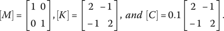
Also, the system responses {X} and ![]() are given by:
are given by:
and
where x1 and x2 are the displacements of masses 1 and 2.
Accordingly, the active and reactive powers can be determined from:
Figure 12.3 displays the active and reactive powers as function of the excitation frequency ω.
Note that the system has eigenvalues of 1 and 3, that is, natural frequencies of 1 and 1.732 rad s−1 and that the reactive power vanishes at 1 and 1.732 rad s−1 as shown in Figure 12.3.

Figure 12.2 Multi‐spring‐damper‐mass system.

Figure 12.3 Active and reactive power of multi‐spring‐damper‐mass system.
12.3 Vibrational Power Flow in Beams
The power flow in beams can be predicted using a finite element model of the entire beam system, in the global coordinate system, is used to generate the overall stiffness [K], mass [M], and damping [C] matrices of the beam assembly after accounting for the boundary conditions.
The resulting model is then utilized along with the applied load vector {F} to compute the nodal deflection vector {X} such that:
where ω is the frequency of a sinusoidal excitation acting on the beam.
The nodal deflection vector {X} is then used to extract the deflection vectors {Xe} for the individual elements where e = 1, … , N with N denoting the total number of elements. Note that ![]() with w and w,x denoting the transverse and angular deflection. Also, i and j define the nodes bounding the eth element as shown in Figure 12.4.
with w and w,x denoting the transverse and angular deflection. Also, i and j define the nodes bounding the eth element as shown in Figure 12.4.

Figure 12.4 Finite element of a beam.
Now, the local force vector {Fe} acting on the eth beam element can be determined from:
where [Ke], [Ce], and [Me] are the stiffness, damping, and mass matrices of the eth element. The stiffness and mass matrices are as given in Chapter 4.
Note also that {Fe} = {Vi Mi Vj Mj}T with Vi,j and Mi,j denoting the shear and bending moments acting at nodes i and j as shown in Figure 12.4.
Then, the structural intensity ![]() of the eth element is given by:
of the eth element is given by:
with ![]() and
and ![]() denoting the active and reactive powers of the eth element.
denoting the active and reactive powers of the eth element.
Solution
The beam/ACLD system is divided into 32 elements. The first three natural frequencies of the uncontrolled system are 48.9, 248.4, and 667.8 Hz, respectively.
Figure 12.6 shows the frequency response of the beam when it is fully treated with the ACLD and subject to unit end transverse load. The figure displays a comparison between the response of the uncontrolled beam and that of the beam when it is controlled using a velocity feedback gain KD = 7.4. It is evident that considerable attenuation of the first three modes is achieved.
Figure 12.7 shows the corresponding active power flow of the fully treated beam as a function of the excitation frequency. The figure indicates that the power flow attains a maximum at the resonant frequencies. Furthermore, it is clear that the power flow is considerably reduced with the velocity feedback. Such a reduction is attributed to the attenuation of the beam vibration.
The power flow, along the beam, are shown in Figures 12.8 through 12.10 for three different excitation frequencies (48.9, 248.4, and 667.8 Hz) that correspond to the first three natural frequencies of the beam/ACLD composite. The figures show also comparisons between the open‐loop (KD = 0.0) and closed‐loop (KD = 7.4) characteristics. It is important to note that it is evident that the spatial profile of the power flow, at any particular mode of vibration, is to some extent similar to the corresponding mode shape of the beam. Also, note that there is a significant attenuation of the net power flow due to the activation of the ACLD controller when KD = 7.4.
Furthermore, it is evident that the computed power flow distributions are in close agreement with the distributions as predicted by using ANSYS software package.
Computation of the power flow over the beam/passive constrained layer damping (PCLD) assembly is carried out according to the procedure outlined in Appendix 12.A.
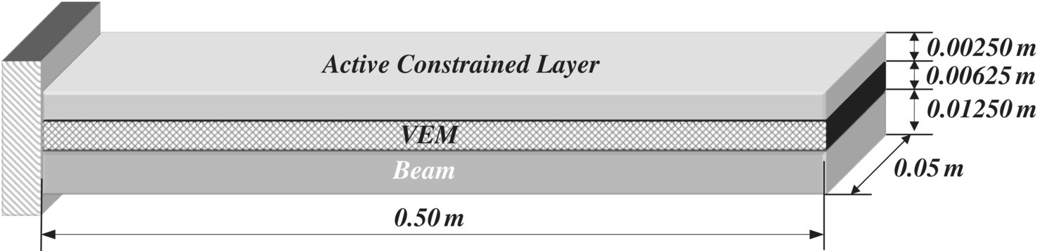
Figure 12.5 Beam with ACLD treatment.

Figure 12.6 Open and closed‐loop frequency response functions of a fully treated beam.

Figure 12.7 Open and closed‐loop active power flow of fully treated beam.

Figure 12.8 Open and closed‐loop power flow of fully treated beam at the first mode (48.9 Hz).

Figure 12.9 Open and closed‐loop power flow of fully treated beam at the second mode.

Figure 12.10 Open and closed‐loop power flow of fully treated beam at the third mode.
Table 12.1 Physical properties of the base beam and the viscoelastic materials.
| Material | Length (m) | Thickness (m) | Width (m) | Density (kg m−3) | Young's modulus (MPa) |
| Beam | 0.5 | 0.012 5 | 0.05 | 7800 | 210,000 |
| VEM | 0.5 | 0.006 25 | 0.05 | 1104 | 60 |
Table 12.2 Physical properties of the piezoelectric constraining layer.
| Length (m) | Thickness (m) | Width (m) | Density(kg m−3) | Young'smodulus (MPa) | d31(m V−1) | k31 | g31(Vm N−1) | k3t |
| 0.5 | 0.0025 | 0.05 | 7600 | 63 | 186E‐12 | 0.34 | 116E‐2 | 1950 |
12.4 Vibrational Power of Plates
12.4.1 Basic Equations of Vibrating Plates
In this section, the emphasis is placed on presenting the basic equations that govern the vibration of a thin flat plate based on the classical Kirchhoff assumptions (Rao 2007). Under these assumptions, the plate thickness h is assumed to be small as compared to the plate's length and width (a and b), whereas the transverse deflection w is considered comparable to h. Furthermore, the plate thickness is assumed to be uniform and symmetric about the mid‐surface so that three‐dimensional stress effects are ignored.
Figure 12.11 displays a schematic drawing of a Kirchhoff plate along with the in‐plane normal forces Ni, in‐plane shear forces Nij, bending moments Mi, twisting moments Mij acting on it, and transverse shear forces Qi.

Figure 12.11 Forces and moments acting on a Kirchhoff plate.
Expressions of these forces and moments are given by (Rao 2007) as follows:
- In‐Plane Normal Forces (Ni)
(12.20)

where E is Young's modulus of the plate, ν is its Poisson's ratio, z is the distance from the mid‐surface, and w,ii is the second spatial derivative of the deflection with respect to i (i = x, y).
- In‐Plane Shear Forces (Nij)
(12.21)

where G is the shear modulus of the plate.
- Bending Moments (Mi)
(12.22)

where D is the flexural rigidity of the plate, given by: D = Eh3/(12[1 − ν2]).
- Twisting Moments (Mij)
(12.23)

- Transverse Shear Forces (Qi)
(12.24)

Note that all these forces and moments are function of the transverse deflection w and its spatial derivatives with respect to x and y. In a finite element formulation, the transverse deflection can be replaced by the classical interpolation representation w = [N]{Δe} in terms of the interpolating function [N] and the nodal deflection vector {Δe}.
12.4.2 Power Flow and Structural Intensity
The structural intensity (I) is the vibrational power flow (SP) per unit cross‐sectional area of a dynamically loaded elastic plate. The net power flow or active intensity in a two‐dimensional plate‐like structure with a steady‐state vibration is given by (Xu et al. 2005):

where Ii(ω), σik(ω), and ![]() denote the structural intensity in the ith direction, the stress in the ikth directions, and the complex conjugate of the velocity in the kth direction, respectively. Also, Re(.) denotes the real part of (.).
denote the structural intensity in the ith direction, the stress in the ikth directions, and the complex conjugate of the velocity in the kth direction, respectively. Also, Re(.) denotes the real part of (.).
The structural intensity for a quadrilateral plate element can be expressed in the form of power flow per unit width. The x and y components of structural intensities can be expressed as

where Im, Ni, Mi, Mij, and Qi denote the imaginary part, in‐plane forces, bending moment, twisting moment, and transverse shear forces per unit width, respectively. Also, u*, v*, and w* are the complex conjugate velocities in the x, y, and z directions. Furthermore, ![]() is the complex conjugate of the angular displacement about the ith direction.
is the complex conjugate of the angular displacement about the ith direction.
For a particular plate‐like structure, the structural intensity components (Ix and Iy) can be computed and maps of the contours of the structural intensity can be plotted.
Equally important are “the streamline” maps that display the flow as lines everywhere parallel to the velocity field. The relative spacing of the lines indicates the speed of the flow. The structural intensity streamline can be mathematically expressed as (Xu et al. 2005):

where r is the energy flow particle position vector.
Thus, for the case of the two‐dimensional plate‐like structures, the differential equation describing a streamline, in a plane perpendicular to the k direction, is given by:

Equation (12.28) defines the differential equation ![]() that describes the streamline.
that describes the streamline.
Solution
For the cantilever plate under consideration, the first natural frequency as computed by the FEM is found to be 28.73 Hz. The corresponding mode shape is displayed in Figure 12.13.
- C1 = 2000 Ns m−1 and C2 = 2000 Ns m−1.
For this case, the transverse deflection distribution map of the plate is shown in Figure 12.14. The figure indicates that the maximum deflection is confined to the area close to the excitation. However, the deflection is minimized near and past the locations of the dampers C1 and C2.
Figures 12.15 and 12.16 display the corresponding structural intensity and streamline maps. The maps indicate that the vibration energy flows from the excitation source to the dampers that act as energy sinks. Note that as the values of C1 and C2 are equal, then the energy flows are distributed equally from the energy source to the sinks as is displayed clearly in Figures 12.15 and 12.16.
- C1 = 2000 Ns m−1 and C2 = 20,000 Ns m−1.
Figures 12.17 and 12.18 display the corresponding power flow and streamline maps for this case. The power flow map of Figure 12.17 indicates that the vibration energy flows from the excitation source primarily to the damper with the low damping coefficient (C1) whereas the structural intensity is almost blocked completely at the damper with the high damping coefficient (C2). This conforms with conclusions following Eq. (12.16).
The streamline map of Figure 12.18 illustrates clearly that the structural intensity has been steered toward the damper with the low damping coefficient (C1). Hence, if a critical object, such as a payload or an instrument, is located near the damper C2, then increasing its damping coefficient tends to redirect the vibration energy away from it to avoid undesirable excitation from reaching it.
- C1 = 20,000 Ns m−1 and C2 = 2000 Ns m−1.
Figures 12.19 and 12.20 display the corresponding structural intensity and streamline maps for this case. The maps indicate that increasing the value of C1 and decreasing that of C2 results in reversing the wave transmission path as compared to case (b).
This suggests that, with appropriate control of the damping coefficients, it would be possible to steer the wave propagation direction as needed. More importantly, by monitoring the instantaneous power flow at a particular location, it is possible to adaptively control the damping coefficients of the dampers to drive the power flow at this location to a minimum value using, for example, the Least Mean Square (LMS) control algorithm.

Figure 12.12 Schematic drawing of a damped cantilever plate system.

Figure 12.13 The mode shape of the first natural frequency of the cantilever plate system.

Figure 12.14 The transverse deflection map of the cantilever plate system at the first natural frequency.

Figure 12.15 The structural intensity distribution map of the cantilever plate system at the first natural frequency (C1 = 2000 Ns m−1 and C2 = 2000 Ns m−1).

Figure 12.16 The streamlines distribution map of the cantilever plate system at the first natural frequency (C1 = 2000 Ns m−1 and C2 = 2000 Ns m−1).

Figure 12.17 The structural intensity distribution map of the cantilever plate system at the first natural frequency (C1 = 2000 Ns m−1 and C2 = 20,000 Ns m−1).

Figure 12.18 The streamlines distribution map of the cantilever plate system at the first natural frequency (C1 = 2000 Ns m−1 and C2 = 20,000 Ns m−1).

Figure 12.19 The structural intensity distribution map of the cantilever plate system at the first natural frequency (C1 = 20,000 Ns m−1 and C2 = 2000 Ns m−1).

Figure 12.20 The streamlines distribution map of the cantilever plate system at the first natural frequency (C1 = 20,000 Ns m−1 and C2 = 2000 Ns m−1).
Solution
Figure 12.21a,b show the power flow distributions over the plate as computed by the MATLAB FEM and ANSYS software packages, respectively, when the damping coefficients C1 = 5 Ns m−1 and C2 = 5 Ns m−1.
It is evident that there is a close agreement between the predictions of the MATLAB FEM and ANSYS software.
When the damping coefficients become C1 = 1 Ns m−1 and C2 = 5 Ns m−1, Figure 12.22a,b emphasizes the close agreement between the power flow distributions over the plate as predicted by the MATLAB FEM and ANSYS software packages, respectively.

Figure 12.21 The power flow distribution maps of the cantilever plate system at the first natural frequency (C1 = 5 Ns m−1 and C2 = 5 Ns m−1).

Figure 12.22 The power flow distribution maps of the cantilever plate system at the first natural frequency (C1 = 1 Ns m−1 and C2 = 5 Ns m−1).
12.4.3 Control of the Power Flow and Structural Intensity
The active vibrational power flow (P), at a particular location, can be controlled by adaptively adjusting the damping coefficients of the dampers, as shown schematically in Figure 12.23, to drive the power flow at this location to a minimum value using, for example, the LMS control algorithm.

Figure 12.23 Controller of the power flow of a damped plate system.
In order to develop the control algorithm, the equation of motion of a vibrating system excited at one of its natural frequencies, as given by Eq. (12.8), reduces to:
Substituting Eq. (12.29) into Eq. (12.13), yields the following expression of the active power flow PFi:
Hence, for a constant excitation {F}, the active power flow is inversely proportional to the damping matrix [C]. This statement is supported by the conclusions of Example 12.1 as quantified by Eq. (12.16).
For a plate system that is damped by N discrete dampers, the damping matrix [C] is a diagonal matrix, and hence Eq. (12.30) reduces to:

where Cj denotes the damping coefficient of the jth discrete damper. Also, the coefficients ![]() where fj denotes the coefficient of the excitation force vector{F}.
where fj denotes the coefficient of the excitation force vector{F}.
In order to design the power flow controller, a performance index J is defined such that:
where e denotes the power flow error. Also, PFr defines a desirable final value of the power flow.
The damping coefficients of the dampers are selected to minimize the performance index resulting in effect in a LMS control action. The LMS algorithm is a gradient‐based algorithm that is commonly used in adaptive signal processing (Widrow and Stearns 1985). The LMS controller updates iteratively the damping coefficients of the dampers by moving along the direction of the negative gradient ∇J of J such that the damping coefficients at the k + 1th iteration are determined in terms of the damping coefficients at the kth iteration as follows:
where α is the step size such that α > 0. From Eqs. (12.31) and (12.32), Eq. (12.33) reduces to:

where Ai = 2α ai = constant > 0.
Accordingly, Eq. (12.34) can be used to generate the block diagram of the power flow control system as shown in Figure 12.24.

Figure 12.24 Block diagram of the controller of the power flow of a damped plate system.
Solution
The LMS controller presented in Section 12.4.3 is implemented using Ai = 0.5E20, PFr = 5E‐14 Nm s−1, C1 = 100 Ns m−1, and C2 = 1000 Ns m−1.
Figure 12.26 displays the effect of the iteration number k on the adaptive characteristics of the controller as quantified by the value of the coefficient of damping C1 and the resulting objective function J. It can be seen that, as the iteration number increases, the objective function decreases, and the damping coefficient C1 increases. More importantly, as k increases, the direction of the power flow can be steered and redirected from flowing toward the damper C1 (when k = 0 and C1 = 100 Ns m−1) to flowing toward the damper C2 (when k = 5000 and C1 = 6000 Ns m−1). In this manner, the power flow direction at the sensor location is not only altered, but also minimized to assume a minimum value of (1 − PFi/PFr)2 = 0.5.

Figure 12.25 Schematic drawing of the location of the dampers and power flow sensor for a damped cantilever plate system.

Figure 12.26 Schematic drawing of the location of the dampers and power flow sensor for a damped cantilever plate system.
12.4.4 Power Flow and Structural Intensity for Plates with Passive and Active Constrained Layer Damping Treatments
In this section, the power flow analysis presented in Section 12.4.2 is extended and applied to predict the energetics of plates treated with different configurations of passive (PCLD) and ACLD treatments. Such an approach can be employed to the design of optimal layout and control strategies of the treatments in order to steer the vibration energy and the wave propagation as deemed essential to avoid undesirable excitations from reaching critical locations over the plate structure.
The presented approach is guided by the work of Castel et al. (2012) for structures with PCLD treatments and Alghamdi and Baz (2002) for structures with ACLD treatments.
Three examples are presented here to illustrate the applicability and utility of power flow analysis in studying the energetics of structures treated with PCLD and ACLD treatments. The first example deals with a plate with a single PCLD treatment, the second example considers two PCLD treatments whereas the third example presents the performance of the plate when it is treated with two separately controlled ACLD treatments.
Solution
Figure 12.28 displays the first three modes and corresponding mode shapes of vibration of the plate/PCLD treatment. Figure 12.29 shows the map of the streamlines of the power flow when the plate is excited at its first natural frequency of 72 Hz.
Note that the active power flows toward the front of the PCLD patch and then stopped near the front edge of the patch and redirected to flow inward toward the side edges of the patch.

Figure 12.27 Schematic drawing of a cantilever plate treated with a PCLD patch.

Figure 12.28 Mode shapes of a cantilever plate treated with a PCLD patch at the first three modes.

Figure 12.29 The streamlines distribution map of the cantilever plate/PCLD system at the first natural frequency.
Solution
Figure 12.31 shows the map of the streamlines of the power flow when the plate is excited at its first natural frequency of 72 Hz. With two PCLD treatments, the streamlines are symmetric and flow from the excitation source to the PCLD treatments.

Figure 12.30 Schematic drawing of a cantilever plate treated with two PCLD patches.

Figure 12.31 The streamlines distribution map of the cantilever plate treated with two PCLD patches at the first natural frequency.
Solution
Figure 12.32 shows the maps of the quivers and streamlines of the power flow when the plate is excited at its first natural frequency of 72 Hz. The maps are obtained when both patches are controlled with K1 = K2 = 500 V s m−1. Under such control strategy, the streamlines are also symmetric, as in the case of the PCLD in Example 12.6, and the vibration energy flows from the excitation source directly to the ACLD treatments.
Figure 12.33 shows the corresponding maps of the quivers and streamlines of the power flow when K1 = 0 and K2 = 500 V s m−1 with the excitation maintained at the first natural frequency of 72 Hz. Under such a control strategy, the power flow and streamline flows from the excitation source directly to the bottom ACLD treatment.
The reverse occurs when the control gains are switched such that K1 = 500 and K2 = 0 V s m−1 as shown in Figure 12.34. In this case, the power flow and streamline flows from the excitation source directly toward the top ACLD treatment.
Hence, by proper control of the ACLD patches, it is demonstrated that the wave propagation, as quantified by the power flow and streamlines, can be steered over the plate surface as desired.

Figure 12.32 The power flow (a) and streamlines (b) distribution maps of the cantilever plate treated with two ACLD patches at the first natural frequency when K1 = K2 = 500 V s m−1.

Figure 12.33 The power flow (a) and streamlines (b) distribution maps of the cantilever plate treated with two ACLD patches at the first natural frequency when K1 = 0 and K2 = 500 V s m−1.

Figure 12.34 The power flow (a) and streamlines (b) distribution maps of the cantilever plate treated with two ACLD patches at the first natural frequency when K1 = 500 and K2 = 0 V s m−1.
Solution
Figure 12.36 displays the power flow distributions maps for three different combinations of the shunting resistances connected to the two piezo‐patches as predicted by using ANSYS.
Figure 12.36a shows the power flow distribution over the plate surface when the two patches are shunted with resistors R1 = ∞ Ω (i.e., open circuit) and R2 is set equal to the optimum value ![]() that maximizes the damping ratio corresponding to the first mode of 24.14 Hz. The figure indicates that the power flow distribution near the bottom piezo‐patch with R2 shunting attains its minimal levels. It is evident that the power flows from the excitation source to the optimized energy sink.
that maximizes the damping ratio corresponding to the first mode of 24.14 Hz. The figure indicates that the power flow distribution near the bottom piezo‐patch with R2 shunting attains its minimal levels. It is evident that the power flows from the excitation source to the optimized energy sink.
The reverse becomes true when the top piezo‐patch is shunted with the optimal resistance R1 that maximizes the damping ratio of the first mode while the resistors R2 = ∞ Ω as shown in Figure 12.36c.
When both patches are shunted with optimal resistors, the power flow distribution is minimized all over the plate surface as indicated in Figures 12.36b and 12.37.

Figure 12.35 The plate with shunted piezo‐patches along with the location of the input excitation.

Figure 12.36 The power flow distribution maps of the cantilever plate treated with two piezo‐patches with different shunting strategies.

Figure 12.37 Configuration of the shell/PCLD assembly.
12.5 Power Flow and Structural Intensity for Shells
In this section, the power flow analysis presented in Section 12.4.2 is extended and applied to predict the distribution of power flow over the surface of shell treated with patches of PCLD.
The equations of the structural power flow can be calculated using the approach outlined by Pavic (1990), Gavric and Pavic (1993), Williams (1991), and Ruzzene and Baz (2000). In this approach, the structural intensity for the quadrilateral shell element, shown in Figures 4.32 and 7.37, can be expressed in the form of power flow per unit width. The x and y components of structural intensities can be expressed as

where Ni, Mi, Mij, and Qi denote the in‐plane forces, bending moment, twisting moment, and transverse shear forces per unit width, respectively. Also, u*, v*, and w* are the complex conjugate velocities in the x, y, and z directions. Furthermore, ![]() is the complex conjugate of the angular displacement about the ith direction.
is the complex conjugate of the angular displacement about the ith direction.
Alternatively, the power flow SP can also be calculated directly from the finite element model using Eq. (12.9) such that:

Note that with the excitation at one of the modes of vibration the reactive power QF vanishes and the active power PF quantifies the total structural power. This approach enables the use of both the FEM developed in Sections 4.8 and 7.5 as well as the ANSYS FEM in Appendix 12.A.
Solution
Figure 12.38a displays the power flow distributions maps for the shell/PCLD as predicted by using the FEM described in Sections 4.8 and 7.5.
Figure 12.38b shows the corresponding mode shape of the shell at the first mode of vibration of 60 Hz. It is evident the close correspondence between the power flow distribution and the mode shape of the vibrating shell.
Figure 12.39 displays the finite element mesh of ANSYS software package indicating the shell, the PCLD patches, and the location of the external excitation.
Figure 12.40 displays the power flow distributions maps for the shell/PCLD as predicted by using ANSYS. It is evident the close agreement between the MATLAB predictions shown in Figure 12.38a and ANSYS predictions shown in Figure 12.40.


Figure 12.38 The power flow distribution map over the cantilever shell treated with two PCLD patches using MATLAB FEM approach.

Figure 12.39 The finite element mesh of the shell/PCLD assembly using ANSYS.

Figure 12.40 The power flow distribution map over the cantilever shell treated with two PCLD patches using ANSYS.
12.6 Summary
This chapter has presented the analysis of the power flow over vibrating structures in the presence of various types of damping including: classical viscous damping, VEM in constrained configurations, passive as well as ACLD, and shunted piezoelectric patches.
The chapter has presented also the concept of using vibration damping element in steering the power flow over the structure passively or actively using adaptive control algorithm.
References
- Alfredsson, K. (1997). Active and reactive structural energy flow. ASME Journal of Vibration and Acoustics 119: 70–79.
- Alfredsson, K., Josefson, B., and Wilson, M. (1996). Use of the energy flow concept in vibration design. AIAA Journal 34 (6): 750–755.
- Alghamdi A. A. A. and Baz A., “Power flow in beams treated with active constrained layer damping,” Proceedings of the 6th Saudi Engineering Conference, KFUPM, Dhahran, Vol. 5, pp. 445–460, 2002.
- Bouthier, O. and Bernhard, R. (1995). Simple models of energy flow in vibrating membranes. Journal of Sound and Vibration 182 (1): 79–147.
- Castel, A., Loredo, A., El Hafidi, A., and Martin, B. (2012). Complex power distribution analysis in plates covered with passive constrained layer damping patches. Journal of Sound and Vibration 331 (11): 2485–2498.
- Gavric, L. and Pavic, G. (1993). A finite element method for computation of structural intensity by the normal mode approach. Journal of Sound and Vibration 164 (1): 29–43.
- Gibbs, G., Fuller, C., and Silcox R. (1993). Active Control of Flexural and Extensional Power Flow in Beams Using Real Time Wave Vector Sensors. Second Conference on Recent Advances in Active Control of Sound and Vibration, April 28–30.
- Halkyard, C. and Mace, B. (1995). Structural intensity in beams – waves, transducer systems and the conditioning problem. Journal of Sound and Vibration 185 (2): 279–298.
- Linjama, J. and Lahti, T. (1992). Estimation of bending wave intensity in beams using the frequency response technique. Journal of Sound and Vibration 153 (1): 21–36.
- Lyons, R. (1975). Statistical Energy Analysis of Dynamical Systems: Theory and Applications. Cambridge, MA: MIT Press.
- Mandal, N.K. and Biswas, S. (2005). Vibration power flow: a critical review. The Shock and Vibration Digest 37 (1): 3–11.
- Mandal, N.K., Rahman, R.A., and Leong, M.S. (2003). Structure‐borne power transmission in thin naturally orthotropic plates: general case. Journal of Vibration and Control 9: 1189–1199.
- Nefske, D.J. and Sung, S.H. (1987). Power flow finite element analysis of dynamic systems: Basic theory and applications to beams. Statistical Energy Analysis 3: 47–54.
- Noiseux, D. (1970). Measurement of power flow in uniform beams and plates. The Journal of The Acoustical Society of America 47 (1): 238–247.
- Nouh, M., Aldraihem, O., and Baz, A. (2015). Wave propagation in metamaterial plates with periodic local resonances. Journal of Sound and Vibration 341: 53–73.
- Pavic, G. (1976). Measurements of structure borne wave intensity, part I: formulation of the methods. Journal of Sound and Vibration 49 (2): 221–230.
- Pavic, G. (1987). Structural surface intensity: an alternative approach in vibration analysis and diagnosis. Journal of Sound and Vibration 115 (3): 405–422.
- Pavic, G. (1990). Vibrational energy flow in elastic circular cylindrical shells. Journal of Sound and Vibration 142 (2): 293–310.
- Pavic, G. (2005). The role of damping on energy and power in vibrating systems. Journal of Sound and Vibration 281 (1–2): 45–71.
- Rao, S.S. (2007). Vibration of Continuous Systems. New Hoboken, NJ: Wiley.
- Ruzzene, M. and Baz, A. (2000). Active control of power flow in ribbed and fluid‐loaded shells. Journal of Thin Walled‐Structures 38 (1): 17–42.
- Widrow, B. and Stearns, S. (1985). Adaptive Signal Processing. Englewood Cliffs, NJ: Prentice‐Hall, Inc.
- Williams, E. (1991). Structural intensity in thin cylindrical shells. The Journal of The Acoustical Society of America 89 (4): 1615–1622.
- Williams, E., Dardy, H., and Fink, R. (1985). A technique for measurements of structure‐borne intensity in plates. The Journal of the Acoustical Society of America 78 (6): 2061–2068.
- Wohlever, J. and Bernhard, R. (1992). Mechanical energy flow models of rods and beams. Journal of Sound and Vibration 153 (1): 1–19.
- Xua, X.D., Lee, H.P., Lu, C., and Guo, J.Y. (2005). Streamline representation for structural intensity fields. Journal of Sound and Vibration 280 (1–2): 449–454.
12.A Calculation of Power Flow in ANSYS
In order to estimate the power flow SP in structures, the internal forces and deflections at the different finite element nodes, subject to external excitation, are calculated and substituted in:
where F is the force and δ is the deflection vector.
In case of harmonic excitation, at a frequency ω, SP can be rewritten as
where the force F is replaced by K δ with K denoting the stiffness matrix.
Accordingly, the following procedure illustrates how to develop the power flow distribution in a finite element model of a composite (ACLD) beam, which is excited with harmonic force tuned at the first natural frequency. The procedure is presented using ANSYS APDL (ANSYS Parametric Design Language).
The procedure applied follows the following sequence:
- Step 1: Define all the model parameters
- Step 2: Enter the model creation pre‐processor (/prep7)
- Step 3: Enter the solution processor (/solu)
- Carry out “Modal Analysis” to calculate the natural frequencies.
- Carry out “Harmonic Analysis” by defining excitation load at specified location and with specified amplitude and is oscillating at the natural frequencies calculated in the “Modal Analysis” step.
- Step 4: Enter the database results post‐processor
- Select the load step to post‐process.
- Calculate the elements results for the entire model (stresses and deflections).
- Use the “Element Table” feature to carry out mathematical calculations on the extracted stress/deflection results.
- Plot the power flow distribution over the entire structure.
- Step 1: Prepare the pre‐processor/solver/post‐processor environment:
/title, Power Flow in PCLD beam/UNITS,SI !Specifies the unit system to be used in the model/SHOW,WIN32C !Specifies the device and other parameters for graphics displays/CONT,1,32,AUTO !Specifies the uniform contour values on stress displays./page,15000,,15000,,0, !Defines number of lines per page - Step 2: Start the pre‐processor where the model is being developed; materials are defined and element types selected
/PREP7!*** Define variables to be used in the FE model later!*********************************************************! Geometrical parameters!***********************inch=25.4e-3Lp=0.5 ! length of base beamWp=0.05 ! width of base beamTp=0.0125 ! thickness of base beamLpz=Lp ! length of PZT constraining layerWpz=Wp ! width of PZT constraining layerTpz=0.0025 ! thickness of PZT constraining layerLv=Lp ! length of Viscoelastic (VEM) layerWv=Wp ! width of Viscoelastic (VEM) layerTv=0.00625! thickness of Viscoelastic (VEM) layer! Material properties parameters!*******************************rho_p=7800 ! Density of base beamrho_pz=7600 ! Density of PZT layerrho_v=1104 ! Density of VEM layerE_p=210e9 ! Young’s Modulus of base beamE_v=60e6 ! Young’s Modulus of VEM layerdamp_p=0 ! Damping ratio for base beam materialdamp_pz=0 ! Damping ratio for PZT materialdamp_v=0.5 ! Damping ratio for VEM material characterized with loss factor = 1!*** Element Type and Material Definition!****************************************! Element Types!**************et,1,solid226,1001! Piezoelectric elementet,2,solid186! Solid Element for beam and VEM!*********************************************************! Material Definitions!*********************! Due to the anisotropic nature and coupling effect of piezoelectric materials, they have specific way in defining the structural/electrical material properties matrices. This is done using tabular data for the different matrix entries!*********************************************************/COM, MATERIAL PROPERTIES OF LEAD ZIRCONATE TITANATE (PZT-5A)/COM,/COM, -- MATERIAL MATRICES (POLAR AXIS ALONG Y-AXIS): IEEE INPUT/COM,/COM, [s11 s13 s12 0 0 0 ] [ 0 d31 0 ] [ep11 0 0 ]/COM, [s13 s33 s13 0 0 0 ] [ 0 d33 0 ] [ 0 ep33 0 ]/COM, [s12 s13 s11 0 0 0 ] [ 0 d31 0 ] [ 0 0 ep11]/COM, [ 0 0 0 s44 0 0 ] [ 0 0 d15]/COM, [ 0 0 0 0 s66 0 ] [ 0 0 0 ]/COM, [ 0 0 0 0 0 s44] [d15 0 0 ]/COM,!*********************************************************S11=15.874E-12S12=-4.25E-12S13=-9.49E-12S33=15.87E-11S44=48.9E-12S66=47.3E-12D15=6.67E-10D31=-1.86E-10D33=7.5E-10EP11=4140EP33=4500!*********************************************************! Piezoelectric layers material properties!*****************************************TB,ANEL,1,,,1 ! ANISOTROPIC ELASTIC COMPLIANCE MATRIXTBDA,1,S11,S13,S12TBDA,7,S33,S13TBDA,12,S11TBDA,16,S44TBDA,19,S44TBDA,21,S66TB,PIEZ,1,,,1 ! PIEZOELECTRIC STRAIN MATRIXTBDA,2,D31TBDA,5,D33TBDA,8,D31TBDA,10,D15TB,DPER,1,,,1 ! DIELECTRIC PERMITTIVITY AT CONSTANT STRESSTBDA,1,EP11,EP33,EP11MP,DENS,1,rho_pz ! DENSITY of PZT layerMP,DMPRAT,1,damp_pz!*******************************************************! Base Beam Material Definition!******************************MP,DENS,2,rho_pMP,EX,2,E_pMP,PRXY,2,0.3MP,DMPRAT,2,damp_p! VEM layer Material Definition!******************************MP,DENS,3,rho_vMP,EX,3,E_vMP,PRXY,3,0.499MP,DMPRAT,3,damp_v!**********************************************!**********************************************!*** MODELING!************! Base Beam!***********BLOCK,0,Lp,0,Tp,-Wp/2, Wp/2! VEM Layer!**********BLOCK,0,Lp,Tp,Tp+Tv,-Wv/2, Wv/2! PZT Layer!**********BLOCK,0,Lp,Tp+Tv,Tp+Tv+Tpz,-Wv/2, Wv/2allsel,allvglue,allnummrg,KPnumcmp,all!*********************************************!*** MESHING!***********! Define number of FE divisions for the model lines!***********************************************lsel,s,,,alllsel,u,loc,x,0lsel,u,loc,x,Lplesize,all,,,48lsel,s,loc,x,0lsel,a,loc,x,Lplsel,u,loc,z,Wp/2lsel,u,loc,z,-Wp/2lesize,all,,,1lsel,s,loc,x,0lsel,a,loc,x,Lplsel,r,loc,z,Wp/2lesize,all,,,1lsel,s,loc,x,0lsel,a,loc,x,Lplsel,r,loc,z,-Wp/2lesize,all,,,1allsel,all!***********************************************! Meshing Beam!*************allsel,allvsel,s,,,1VATT, 2,,2,,vsweep, all ! Mesh Volume # 1 (Beam)allsel,all! Meshing VEM!************allsel,allvsel,s,,,2VATT, 3,,2,,vsweep, all ! Mesh Volume # 2 (VEM)allsel,all! Meshing PZT!************allsel,allvsel,s,,,3VATT, 1,,1,11,vsweep, all ! Mesh Volume # 3 (PZT)allsel,all!***************************************************!*** Apply Boundary Conditions!*****************************! Structural Boundary Conditions!*******************************nsel,s,loc,x,0D,all,ux,0D,all,uy,0D,all,uz,0allsel,all! Electrical Boundary Conditions for the PZT layer!*************************************************vsel,s,,,3aslvasel,r,loc,y,Tp+Tvnsla,s,1cp,1,volt,allallsel,allvsel,s,,,3aslvasel,r,loc,y,Tp+Tv+Tpznsla,s,1cp,2,volt,allallsel,allfinish!************************************************* - Step 3: Define the solver parameter, type of analysis, and carry out the solution
/SOLU! Modal Analysis!***************ANTYPE,2 ! Modal analysisMODOPT,LANB,10EQSLV,SPARMXPAND,10, , ,1OUTPR,ALL,ALL,OUTRES,ALL,ALLSOLVE*GET,Mode1_Freq,MODE,1,FREQ,REAL*GET,Mode2_Freq,MODE,2,FREQ,REAL*GET,Mode3_Freq,MODE,3,FREQ,REAL*GET,Mode4_Freq,MODE,4,FREQ,REAL*GET,Mode5_Freq,MODE,5,FREQ,REAL*GET,Mode6_Freq,MODE,6,FREQ,REAL*GET,Mode7_Freq,MODE,7,FREQ,REAL*GET,Mode8_Freq,MODE,8,FREQ,REAL*GET,Mode9_Freq,MODE,9,FREQ,REALFINISH!***************************************************! Harmonic Analysis!******************/SOLUantype,3 ! Harmonic AnalysisHARFREQ,Mode1_Freq,Mode1_Freq,NSUBSET,1KBC,1outres,all,all! Apply Force Excitation!***********************esel,s,mat,,2nsle,s,1nsel,r,loc,x,LpF,all,Fy,1allsel,allsolveFINISH!**************************************************** - Step 4: Post‐process the calculated results
/post1SET,FIRST! Calculate the deflection in the x-direction for the structure elements!*********************************AVPRIN,0, ,ETABLE,disp_x,U,X! Calculate the deflection in the y-direction for the structure elements!*********************************AVPRIN,0, ,ETABLE,disp_y,U,Y! Calculate the deflection in the z-direction for the structure elements!*********************************AVPRIN,0, ,ETABLE,disp_z,U,Z! Calculate Fx!*************AVPRIN,0, ,ETABLE,f_xx,F,X! Calculate Fy!*************AVPRIN,0, ,ETABLE,f_yy,F,Y! Calculate Fz!*************AVPRIN,0, ,ETABLE,f_zz,F,Z! Carry out arithmetic operations!********************************SMULT,en_xx,F_XX,DISP_X,1,1, ! FxuxSMULT,en_yy,F_YY,DISP_Y,1,1, ! FyuySMULT,en_zz,F_ZZ,DISP_Z,1,1, ! Fzuz! Calculate Ix=SQRT[(Fxux)2 + (Fyuy)2 + (Fzuz)2]!******************************SEXP,Ixd2,EN_XX,,2,,SEXP,Iyd2,EN_YY,,2,,SEXP,Izd2,EN_ZZ,,2,,SADD,II1,IXD2,IYD2,1,1, ,SADD,II,II1,IZD2,1,1, ,SEXP,IISQR,II,,0.5,,!************************************************! Plot the power flow distribution!*********************************PLETAB,IISQR,AVG!****************! Bottom View!************/VIEW,1,,-1/ANG,1/REP,FAST
Problems
- 12.1 Consider the four spring‐damper‐mass system shown in Figure P12.1.
If k = 1, m = 1, and the damping matrix = 0.1 stiffness matrix, determine the active and reactive power distributions over the four masses when the first mass is excited sinusoidally by a unit force at the first system natural frequency.

Figure P12.1 Multi‐spring‐damper‐mass system
- 12.2 Consider the fixed‐free rod/VEM system shown in Figure P12.2. The rod is made of aluminum with width of 0.025 m, thickness of 0.025 m, and length of 1 m. The VEM has width of 0.025 m, thickness = 0.025 m, and density of 1100 kg m−3. The storage modulus and loss factor of the VEM are predicted by GHM model with one mini‐oscillator (E0 = 15.3MPa, α1 = 39, ζ1 = 1, ω1 = 19, 058rad/s). Determine the power flow over the rod when it is subjected to a unit sinusoidal force acting at node 3 and the excitation occurs at the first natural frequency of the assembly.
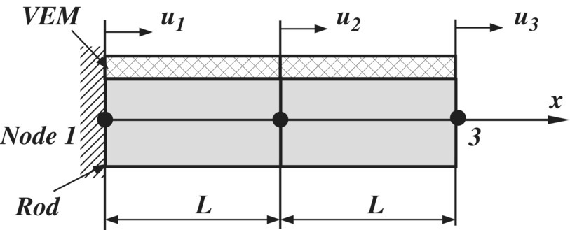
Figure P12.2 Two‐element model a rod/unconstrained VEM. - 12.3 Consider the fixed‐free rod/VEM system shown in Figure 4.11. The rod is made of aluminum with width of 0.025 m, thickness of 0.025 m, and length of 1 m. The VEM has width of 0.025 m, thickness = 0.025 m, and density of 1100 kg m−3. The storage modulus and loss factor of the VEM are as given in Example 4.2. The VEM is constrained by an aluminum constraining layer that is 0.025 m wide and 0.0025 m thick. Using the GHM modeling approach of the VEM with one mini‐oscillator (E0 = 15.3MPa, α1 = 39, ζ1 = 1, ω1 = 19, 058rad/s). Determine the power flow over the rod when it is subjected to a unit sinusoidal force acting at node 3 and the excitation occurs at the first natural frequency of the assembly (Figure P12.3).

Figure P12.3 Two‐element model a rod/constrained VEM. - 12.4 Consider the fixed‐free beam/VEM system shown in Figure P12.4. The physical and geometrical parameters of the beam/VEM system are listed in Table 4.4. The beam is divided into 10 finite elements and is subjected to a force F acting along the transverse direction. Determine the power flow over the beam when it is subjected to a unit sinusoidal force acting at node 11 and the excitation occurs at the first natural frequency of the assembly.
Assume that the complex shear modulus G2 of the VEM is represented by a GHM model with four mini‐oscillators that have the properties listed in Table 4.5 such that:
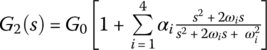 with G0 = 2.72 MPa
Compare the power flow distributions when only two, four, six, and eight elements of the beam are treated with the constrained VEM treatment.

Figure P12.4 Ten‐element cantilever beam with a constrained VEM damping treatment.
- 12.5 Consider the fixed‐free beam/VEM system of Problem 12.4 and shown in Figure P12.4. The properties of the beam, VEM, and an active piezoelectric constraining layer are given in Tables 12.3 and P12.1. Assume that the beam is treated with ACLD over the first five elements. Determine the power flow over the beam, with open‐loop ACLD, when it is subjected to a unit sinusoidal force acting at node 11 and the excitation occurs at the first natural frequency of the assembly.
Determine the power flow distribution also when the ACLD is controlled with a derivative feedback of the position of node 6. Use different values of the control gains and comment on the results.
Table 12.3 Physical and geometrical parameters of beam/VEM system.
Layer Thickness(m) Width(m) Young's modulus(GPa) Density(kg m−3) Poisson'sratio PZT constraining layer h1 = 0.0025 0.025 63 7600 0.3 VEM h2 = 0.0025 0.025 GHM 1100 0.5 Beam h3 = 0.0025 0.025 70 2700 0.3 Table P12.1 Piezo‐constraining layer – PZT.
Parameter d31 – (m V−1) k31 g31 – (Vm N−1) k3t Value 186E‐12 0.34 1.16 1950 - 12.6 Consider the cantilevered flat plate shown in Figure P12.5 that is damped using potentially eight point viscous dampers with damping coefficients C1 through C8. The plate is excited near its fixed end, as shown in the figure, by a unit transverse sinusoidal load at the first natural frequency of the plate.
Determine the structural intensity and the streamline plots of the system for the three arrangements of the point dampers which are listed in Table P12.2.
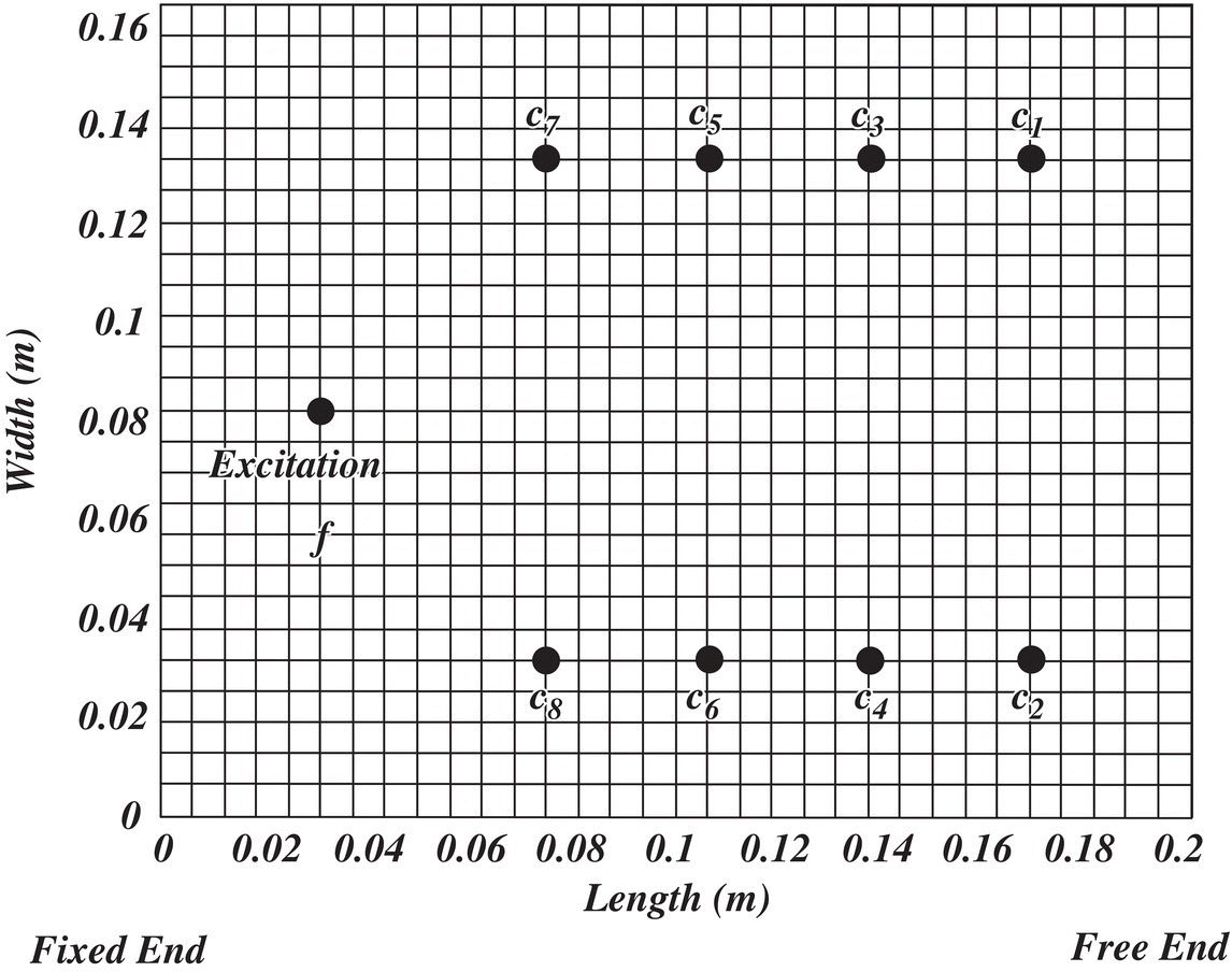
Figure P12.5 Cantilevered plate with eight point dampers.
Table P12.2 Arrangement of point dampers.
Arrangement C1 C2 C3 C4 C5 C6 C7 C8 1 2000 2000 2000 2000 0 0 0 0 2 2000 2000 2000 2000 2000 2000 0 0 3 2000 2000 2000 2000 2000 2000 2000 2000 - Consider the cantilevered beam shown in Figure P12.6 with six periodic sources of internal resonance. The beam is manufactured of assemblies of periodic cells consisting of cavities filled by viscoelastic membranes that support small masses to form sources of local resonance. The geometrical and physical parameters of the beam and the sources of internal resonance are listed in Tables P12.3 and P12.4, respectively. The beam is excited near its free end, as shown in the figure, by a unit transverse sinusoidal load at the first natural frequency of the assembly.
Determine the power flow quiver and the streamline plots of the system.

Figure P12.6 Cantilevered beam with periodic sources of internal resonance.
Table P12.3 Geometrical parameters of the beam with periodic sources of internal resonance.
Length L w h Lc Lr Lg Value (m) 0.3556 0.0635 0.0015 0.0381 0.0127 0.0181 Table P12.4 Physical properties of the beam and damping membranes.
Material Young's modulus (GPa) Poisson's ratio (ν) Density (kg m−3) Aluminum 70 0.30 2700 VEM‐Polyurea 0.02(1 + 0.4i) 0.49 1018 - Consider the 2D metamaterial plate‐like configuration displayed in Figure P12.7. The plate is manufactured of aluminum and consists of assemblies of periodic cells with built‐in local resonances. Each cell is made of a base plate‐like structure that is provided with cavities filled by a viscoelastic membrane that supports a small mass to form a source of local resonance (Nouh et al. 2015). Table 10.6 lists the main geometrical properties of the aluminum plate and the local resonant masses.
The plate is excited near its fixed end, as shown in the figure, by a unit transverse sinusoidal load at the first natural frequency of the assembly.
Determine the power flow quiver and the streamline plots of the system.

Figure P12.7 Cantilevered plate with periodic sources of internal resonance.
- The 2D metamaterial plate‐like configuration displayed in Figure P12.8 is a special case of the plate in Figure 12.7. The plate has only two sources of internal resonance. The main geometrical properties of the aluminum plate and the local resonant masses are as listed in Table 10.6.
The plate is excited near its fixed end, as shown in the figure, by a unit transverse sinusoidal load at the first natural frequency of the assembly.
Determine the power flow quiver and the streamline plots of the system.

Figure P12.8 Cantilevered plate with two sources of internal resonance.
- Consider the clamped‐free shell/PCLD assembly shown in Figure P12.9. The main physical and geometrical parameters of the shell and PCLD are listed in Table P12.5. The shell has an internal radius R is 0.1016 m. The PCLD treatment consists of two patches as displayed in Figure P12.9. The patches are bonded 180° apart on the outer surface of the cylinder with each of which subtending an angle of 90° angle at the center of the shell as shown in Figure P12.9.
Determine the power flow distribution over the shell surface when it is excited sinusoidally by a unit force, at the first natural frequency, at location Ll = 0.9 m using the FEM of Sections 4.8 and 7.5.

Figure P12.9 Configuration of the shell/PCLD assembly.
Table P12.5 Parameters of the shell/ACLD assembly.
Parameter Length (m) Thickness (mm) Density (kg m−3) Young's modulus (GPa) Shell 1.270 0.635 7800 210 VEM 0.600 1.300 1140 a PZT constraining layer 0.600 0.028 7600 66 a G∞ = 292.01 MPa and β∞ = 0.007 for a five‐term GMM of the VEM as described in Example 4.6 and Table 4.6.