
2
Viscoelastic Damping
2.1 Introduction
Viscoelastic damping treatments have been extensively used in various structural applications to control undesirable vibrations and associated noise radiation in a simple and reliable manner (Nashif et al. 1985; Sun and Lu 1995). In this chapter, particular emphasis is placed on studying the dynamic characteristics of such damping treatments and outlining the different mathematical models used to describe the behavior of these treatments over a wide range of operating frequencies and temperatures. Particular focus is given to ascertain the merits and drawbacks of the classical models by Maxwell, Kelvin–Voigt, and Zener (Zener 1948; Flugge 1967; Christensen 1982; Haddad 1995; Lakes 1999, 2009) both in the time and frequency domains.
2.2 Classical Models of Viscoelastic Materials
These models include the of Maxwell, Kelvin–Voigt, and Poynting–Thomson models (Haddad 1995; Lakes 1999, 2009). In these models, the dynamics of ViscoElastic Materials (VEMs) are described in terms of series and/or parallel combinations of viscous dampers and elastic springs as shown in Figure 2.1. The dampers are included to capture the viscous behavior of the VEM, whereas the springs are used to simulate the elastic behavior of the VEM.

Figure 2.1 Classical models of VEMs. (a) Maxwell model, (b) Kelvin–Voigt model, and (c) Poynting–Thomson model.
2.2.1 Characteristics in the Time Domain
The dynamic characteristics of Maxwell and Kelvin–Voigt models in the time domain are summarized in Table 2.1.
Table 2.1 The dynamic equations of Maxwell and Kelvin–Voigt models.
| Model | Maxwell model | Kelvin–Voigt model |
| Stresses and strains of components | 
|

|
| Equilibrium and kinematic equations |
σ = σ s = σ d (2.1) and ε = ε s + ε d (2.3) |
σ = σ s + σ d (2.2) and ε = ε s = ε d (2.4) |
| Constitutive equations | Spring: σ = E
s
ε
s
(2.5) Damper: |
Spring: σ
s
= E
s
ε (2.6) Damper: |
| Model equation | Substituting Eqs. (2.5) and (2.7) into Eq. (2.3) gives: where λ = c d /E s |
Substituting Eqs. (2.6) and (2.8) into Eq. (2.2) gives: |
(E s = Young's modulus of elastic element, c d = damping coefficient of dissipative element)
One can note that the stress–strain equations of the Maxwell and Kelvin–Voigt models can generally be written as follows:
where P and Q are differential operators given by:

Hence, for Maxwell model, p = 1, q = 1, α 0 = 1, α 1 = λ, β 0 = 0 and β 1 = c d while for the Kelvin–Voigt model, p = 0, q = 1, α 0 = 1, β 0 = E s and β 1 = c d .
The ability of both the Maxwell and the Kelvin–Voigt models to predict the characteristics of realistic VEM will be determined by considering the behavior under creep and relaxation loading conditions.
2.2.2 Basics for Time Domain Analysis
The initial and final value theorems of the Laplace transform are essential to the complete understanding of the behavior of viscoelastic models in the time domain. Appendix 2.A summarizes the two theorems and presents the necessary proofs.
Application of these two theorems to Maxwell and Kelvin–Voigt models is summarized in Tables 2.2 and 2.3 when these models are subjected to creep and relaxation loading, respectively. These two theorems provide the means for determining the initial and final limits of the VEM response under different loading conditions. This feature enables the correct calculation of the time response, between these two limits, when the differential equations describing these models are solved as will be demonstrated later.
Table 2.2 Initial and final values of stresses and strains of Maxwell and Kelvin–Voigt models when subjected to creep loading.
| Model | Maxwell model | Kelvin–Voigt model |
| Model | ||
| Loading conditions | The stress is constant σ = σ
0 and the initial and final values of the strain ε are predicted. |
|
| The strain in the Laplace s domain | ||
| Initial value | 
|

|
| Final value | 
|

|
Table 2.3 Initial and final values of stresses and strains of Maxwell and Kelvin–Voigt models when subjected to relaxation loading.
| Model | Maxwell model | Kelvin–Voigt model |
| Model | ||
| Loading conditions | The strain is constant ε = ε
0 and the initial and final values of the stress σ are predicted. |
|
| The stress in the Laplace s domain | ||
| Initial value | 
|

|
| Final value | 
|

|
Table 2.2 indicates that the Maxwell model experiences an initial strain when the creep load is applied, which is typical in VEMs. However, this strain tends to become unbounded as time grows. This feature is not observed or supported experimentally. As for the Kelvin–Voigt model, the initial value theorem indicates zero initial strain, which is rather unrealistic and a bounded final strain of σ 0/E s that is observed in a realistic VEM.
Table 2.3 indicates that the Maxwell model experiences an initial stress when the relaxation strain is applied and that stress is completely relieved as time progresses. Both of these characteristics are typical in VEM. As for the Kelvin–Voigt model, the initial and the final values remain constant E s ε 0, which is rather unrealistic behavior of a VEM.
2.2.3 Detailed Time Response of Maxwell and Kelvin–Voigt Models
Tables 2.4 and 2.5 summarize the detailed behavior characteristics of Maxwell and Kelvin–Voigt models in the time domain between the initial and final values predicted in Tables 2.2 and 2.3.
Table 2.4 The creep characteristics of Maxwell and Kelvin–Voigt models.
| Model | Maxwell model | Kelvin–Voigt model |
| Loading conditions | The stress is constant σ = σ
0 and the time history of the strain is predicted |
|
| Response |

|
|
| Unloading Conditions | The stress is reduced back to zero at time t = t
1
and the time history of the strain |
|
| Response |
with solution ε = ε 1= constant (2.15) 
|
with solution 
|
Table 2.5 Relaxation characteristics of Maxwell and Kelvin–Voigt models.
| Model | Maxwell model | Kelvin–Voigt model |
| Loading conditions | The strain is constant ε = ε
0 and determines the time history of the stress |
|
| Response |

|

|
Tables 2.4 and 2.5 indicate that the Maxwell model predicts unrealistic creep characteristics as the strain tends to be unbounded even for finite stress levels or the strain tends to remain constant when the stress is removed. The Kelvin–Voigt model also yields unrealistic relaxation characteristics with the stress remaining constant with time, indicating that the VEM does not exhibit any stress relaxation. Therefore, neither the Maxwell nor the Kelvin–Voigt model replicates the behavior of realistic VEM.
Note that these predictions, particularly at t = 0, are in agreement with the predictions of the initial and final value theorems listed in Tables 2.2 and 2.3.
In order to avoid the drawbacks and limitations of both the Maxwell and Kelvin–Voigt models, several other spring‐damper arrangements have been considered. For example, a damper with series and parallel springs is considered to combine the attractive attributes and compensate for the deficiencies of both the Maxwell and Kelvin–Voigt models. The resulting model is the Poynting–Thomson model, shown in Figures 2.1c and 2.2a. Other common models are also displayed in Figure 2.2 such the “three‐parameter model” and the “standard solid model” (Zener 1948).

Figure 2.2 Other common viscoelastic models. (a) Poynting–Thomson model, (b) Zener model, (c) Jeffrey model, and (d) Burgers model.
Figure 2.3a,b show the most widely used spring‐mass configurations of VEM models that are employed extensively, particularly, in commercial finite element packages. These two configurations are, namely, the generalized Maxwell model and the generalized Kelvin–Voigt model.

Figure 2.3 Generalized Maxwell (a) and Kelvin–Voigt (b) models.
These two generalized n classical models are assembled in parallel or series to model the complex behavior of realistic VEMs. These models are augmented with additional springs E 0 , either in parallel or series, to eliminate the drawbacks associated with the classical models as outlined in Tables 2.2–2.5.
2.2.4 Detailed Time Response of the Poynting–Thomson Model
The stress σ across the series spring of the Poynting–Thomson model, shown in Figure 2.4, is given by:
and the stress σ across the damper and the parallel spring is given by:

Figure 2.4 Poynting–Thomson viscoelastic model.
Using the Laplace transformation, yields
Hence, the total strain ε across the Poynting–Thomson model is

In the time domain, this equation becomes
From Eqs. (2.11), (2.12), and (2.23), p = 1, q = 1, α 0 = (E s + E p ), α 1 = c d , β 0 = E s E p , and β 1 = E s c d .
- The creep characteristics of the Poynting–Thomson model are obtained as follows:
-
Determine the initial and final values strain:
For stress σ = σ 0, then Eq. (2.22) reduces to:

Then,

and

where
 .
. -
Determine the time history of the strain:
The time history of the strain is determined by solving Eq. (2.23) such that at t = 0, σ = σ 0, and the initial strain ε 0 = σ 0/E s . Hence, Eq. (2.23) reduces to:

This equation has a solution:
where λ = c d /E p and E ∞ = E s E p /(E s + E p ). Note that Eq. (2.24) has the initial and final values ε 0 and ε ∞ at t = 0 and t = ∞.
Figure 2.5 shows the strain–time characteristics as predicted by Eq. (2.24).
-
Determine the initial and final values strain:
- The Relaxation characteristics of the Poynting–Thomson model are obtained as follows:
-
Determining the initial and final values stress:
For strain ε = ε 0, then Eq. (2.22) reduces to:

Then,

and

where
 .
. -
Determining the time history of the stress:
The time history of the stress can be determined by solving Eq. (2.23) such that at t = 0, ε = ε 0, and the initial stress σ 0 = E s ε 0. Hence, Eq. (2.23) reduces to:

This equation has the following solution:
where
 .
.
-
Determining the initial and final values stress:


Figure 2.5 The creep characteristics of the Poynting–Thomson model.
Figure 2.6 shows the stress–time characteristics as predicted by Eq. (2.25).

Figure 2.6 The relaxation characteristics of the Poynting–Thomson model.
Table 2.6 summarizes the main characteristics of Maxwell, Kelvin–Voigt, and Poynting–Thomson models.
Table 2.6 Time domain characteristics of classical viscoelastic models.
| Parameter | Maxwell | Kelvin–Voigt | Poynting–Thomson |
| Model | 
|

|

|
| Dynamic equations | |||
| Creep characteristics | 
|

|

|
| Comments | Unrealistic | Realistic | Realistic |
| Relaxation characteristics | 
|

|

|
| Comments | Realistic | Unrealistic | Realistic |
The characteristics summarized in Table 2.6 ascertain the ability of the Poynting–Thomson model to simulate a realistic behavior of VEMs. However, several combinations of Poynting–Thomson models are necessary to replicate the behavior of realistic VEMs.
Solution
Table 2.7 lists the solutions of the constitutive equations of Maxwell and Kelvin–Voigt models for the given loading and unloading cycle.
Figure 2.8a,b displays the stress–strain characteristics of the Maxwell and Kelvin–Voigt models. The figures indicate that, according to the Maxwell model, the VEM is stiffer and dissipates less energy, as represented by the enclosed area, than that predicted by the Kelvin–Voigt model.

Figure 2.7 A ramp creep loading and loading cycle.

Figure 2.8 Stress–strain characteristics of Maxwell and Kelvin–Voigt models. (a) Maxwell model and (b) Kelvin–Voigt model.
Table 2.7 Solutions of the constitutive equations.
| Parameter | Maxwell | Kelvin–Voigt |
| Constitutive equation | ||
| Equation during loading | ||
| Initial condition (ε 0) | ε 0 = 0 | ε 0 = 0 |
| Response | ε = (ε 0 + 1)e −t − 1 + t | |
| Equation during unloading | ||
| Initial condition (ε 1) | ε 1 = 1.5 | ε 1 = e −1 |
| Response | ε = 3 − t + e −t − 2e 1 − t |
2.3 Creep Compliance and Relaxation Modulus
In Section 2.2, time domain relationships are derived for the different classical VEM models when these models are subjected to creep or relaxation loading. These relationships are obtained by solving the constitutive equations that describe the dynamics of the VEM models subject to initial conditions determined by applying the initial value theorem.
Table 2.8 lists these relationships such that the ratio between the strain and amplitude of the creep stress ε/σ 0 is denoted by the symbol J(t) and called “the creep compliance” and the ratio between the stress and amplitude of the relaxation strain σ/ε 0 is designated by the symbol E(t) and called “the relaxation modulus.”
Table 2.8 The creep characteristics of Maxwell, Kelvin–Voigt, and Poynting–Thomson models.
| Model | Maxwell model | Kelvin–Voigt model | Poynting–Thomson model |
| Creep compliance (J) | 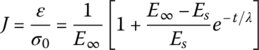
|
||
| Relaxation modulus (E) | 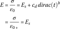 b
b
|
a λ = c d /E s .
b dirac(t) = ∞ at t = 0 and 0 at t = 0+.
It is important to note that these two characteristic properties of VEM are time‐dependent, unlike the corresponding properties for solids, which are constants.
Note also that the process involved in deriving these properties has been tedious and cumbersome as it consists of applying the initial and final value theorems followed by the exhaustive procedure for solving the constitutive equations subject to the initial values and then validating the solution against the obtained final values.
In this section, two other approaches are presented. In the first approach, the direct Laplace and inverse Laplace transformations are applied one after the other to the constitutive equations of the VEM. In the second approach, the topology of the VEM model is translated into a linear set of equations that can be reduced by using the Gauss elimination to determine both J(t) and E(t) simultaneously. The two approaches are implemented in a MATLAB environment to enhance their practicality and utility.
2.3.1 Direct Laplace Transformation Approach
The constitutive equations of the VEM are transformed into the Laplace domain to assume one of the following transfer function forms:
and
When the VEM is subjected to creep loading, the stress σ is replaced by its Laplace transform σ 0/s and Eq. (2.26a) reduces to:
Similarly, when the VEM is subjected to relaxation loading, the strain ε is replaced by its Laplace transform ε 0/s and Eq. (2.26b) reduces to:
The inverse Laplace transform is then used to transform J(s) and E(s) into the time domain creep compliance J(t) and relaxation modulus E(t).
Table 2.9 lists the corresponding creep compliance J(t) and relaxation modulus E(t) for the Maxwell, Kelvin–Voigt, and Poynting–Thomson models.
Table 2.9 Time domain characteristics of classical viscoelastic models.
| Operation | Maxwell | Kelvin–Voigt | Poynting–Thomson |
| Dynamic equations | 
|
||
| Laplace transform of the strain due to creep loading σ 0 | 
|
||
| Inverse Laplace transform of ε/σ 0 = J using MATLAB | >> syms L cd s t
>> ilaplace ((L*s + 1)/(cd*s^2),s,t) J = λ/cd + t/cd |
>> syms L E s t
>> ilaplace(1/(E*s*(L*s + 1)),s,t) J = 1/E − 1/(E * exp(t/λ)) |
>> syms Es Ep cd s t
>> ilaplace (((Es + Ep) + cd*s)/ (s*(Es*Ep+Es*cd*s)),s,t) J = (Ep + Es)/(Ep*Es) ‐ 1/(Ep*exp((Ep*t)/cd)) |
| Laplace transform of the stress due to relaxation loading ε 0 | 
|
||
| Inverse Laplace transform of σ/ε 0 = R using MATLAB | >> syms L cd s t
>> ilaplace ((cd)/(L*s+1),s,t) R = cd/(λ * exp(t/λ)) |
>> syms L E s t
>> ilaplace(E*(L*s + 1)/s,s,t) R = E + E*L*dirac(t) |
>> syms Es Ep cd s t
>> ilaplace((Es*Ep + Es*cd*s)/ (s*(Es + Ep + cd*s)),s,t) R = (Ep*Es)/(Ep + Es) + Es^2/ (exp((t*(Ep + Es))/cd)*(Ep + Es)) |
2.3.2 Approach of Simultaneous Solution of a Linear Set of Equilibrium, Kinematic, and Constitutive Equations
This approach was developed by Vondřejc (2009) and translates the topology of the VEM model into a linear set of equilibrium, kinematic, and constitutive equations which can be reduced by using the Gauss elimination to determine both J and R simultaneously. The approach is implemented in a MATLAB environment to enhance its practicality and utility.
In this approach, the topology of the viscoelastic model is described by N serial strings extending between P points. Each string can consist of a spring and a damper in series. For example, Figure 2.9 shows the description of the topology of the Maxwell and Poynting–Thomson VEM models. In Figure 2.9a, the Maxwell model is described by one string and two points whereas in Figure 2.9b, the Poynting–Thomson model is defined by two strings and three points.

Figure 2.9 Topology of the Maxwell and Poynting–Thomson models. (a) Maxwell model and (b) Poynting–Thomson model.
In a symbolic MATLAB environment, the topology description of the two models is given by the vectors B such that:
Maxwell Model: B = [1, 2, E 1 , cd 1 ],
Poynting–Thomson Model: B = [1, 2, E 1 , inf; 2, 3, E 2 , inf; 2, 3, inf, cd 2 ];
Note that in this description of any string, the component value of a spring or a damper that is missing in the string is set equal to “inf.”
The mathematical formulation of the VEM model, in the Laplace domain, is described as follows:
| Constitutive equations |  (2.28) (2.28) |
| Equilibrium equations | |
| Kinematic equations |
Note that b j and e j denote the beginning and end points of the jth string.
In a matrix form, Eqs. (2.28) through (2.32) take the following form:
where x is a vector of the strains and stresses given by:
where ε j, j + 1 = strain between points j and j + 1, σ i = stress in the ith string, σ = stress applied to the entire VEM topology, and ε = total strain of the entire VEM topology.
Solution
From Eqs. (2.28) through (2.32), the system of equations describing the dynamics of the Maxwell model is given by:

where ![]() .
.
Applying the Gauss elimination method to Eq. (2.35), it reduces to:

Expanding the last row of Eq. (2.36) gives:

Hence, if the VEM is subjected to creep loading such that σ = σ 0, then Eq. (2.37) reduces to:

Using MATLAB symbolic manipulation gives:
Note that the obtained creep compliance J matches that listed in Table 2.9.
Also, if the VEM is subjected to relaxation strain such that ε = ε 0, then Eq. (2.37) reduces to:

Using MATLAB symbolic manipulation gives:
The obtained relaxation modulus E matches that listed in Table 2.9.
2.4 Characteristics of the VEM in the Frequency Domain
Assume a VEM is subjected to sinusoidal stress σ and strain ε, at a frequency ω, such that:
where σ
0 and ε
0 denote the amplitude of the stress and strain, respectively, with ![]() .
.
Hence, for a VEM described by the Maxwell model, Eqs. (2.9) and (2.26b) give:

In a compact form,
where  and
and ![]() . The constitutive equation of the VEM, as given by Eq. (2.41), indicates that the material has a complex modulus E
* = E′[1 + j η] that relates the stress and the strain. Note that:
. The constitutive equation of the VEM, as given by Eq. (2.41), indicates that the material has a complex modulus E
* = E′[1 + j η] that relates the stress and the strain. Note that:
- the real part of the complex modulus = E′ is called the storage modulus,
- the imaginary part of the modulus = E′η is called the loss modulus E″, and
- the ratio between loss and the storage moduli is η is called the loss factor.
Figure 2.10 shows the effect of the excitation frequency on the storage modulus and the loss factor of the Maxwell model.

Figure 2.10 Effect of frequency on the storage modulus and loss factor of Maxwell model. (a) Storage modulus and (b) loss factor.
Note that the Maxwell model indicates that the VEM has zero storage modulus under static conditions (ω = 0) and has a loss factor that is continuously decaying with frequency. These two characteristics contradict the behavior of realistic VEMs.
Figure 2.11 displays graphically the different components of the complex modulus E * = E′[1 + i η].

Figure 2.11 Graphical representation of complex modulus.
Note that the complex modulus makes an angle δ with the real axis such that:
Because of this relationship, the loss factor is also called “tan delta” or the “loss tangent.”
In a similar manner, the constitutive equations for the Kelvin–Voigt and Poynting–Thomson models can be determined in the frequency domain. Table 2.10 lists these equations and gives expressions for the corresponding storage modulus and loss factor for the different models.
Table 2.10 Frequency domain characteristics of classical viscoelastic models.
| Parameter | Maxwell | Kelvin–Voigt | Poynting–Thomson |
| Model | 
|

|

|
| Storage modulus | 
|
E′ = E s |  a
a
|

|

|

|
|
| Comments | Unrealistic | Unrealistic | Realistic |
| Loss Factor | η = 1/ωλ | η = ωλ | η = (β − α)ω/[1 + αβω 2] |

|

|

|
|
| Comments | Unrealistic | Unrealistic | Realistic |
a where ![]() ,
, ![]() , and
, and ![]() .
.
The characteristics summarized in Table 2.10 ascertain the ability of the Poynting–Thomson model to simulate a realistic behavior of VEMs. However, several combinations of Poynting–Thomson models are necessary to replicate the behavior of realistic VEMs.
2.5 Hysteresis and Energy Dissipation Characteristics of Viscoelastic Materials
2.5.1 Hysteresis Characteristics
Consider a VEM subjected to sinusoidal stress σ and strain ε given by
with the stress and strain related by the following constitutive equation
Combining Eqs. (2.43) and (2.44) gives

where σ e = E′ε 0 sin(ωt) and σ d = ηE′ε 0 cos(ωt) denote the elastic and dissipative components of the applied stress σ.
Then σ d can be written as:

Rearranging this equation reduces it to
which is an equation of an ellipse as shown in Figure 2.12a. Figure 2.12b shows a plot of the elastic stress versus the strain and Figure 2.12c combines the elastic and dissipative stress components. Figure 2.12c displays accordingly the total stress σ acting on the VEM versus the strain ε.
Figure 2.12 Stress–strain relationship for a viscoelastic material. (a) dissipative component, (b) elastic component, and (c) viscoelastic material.
Note that the dissipative component takes the form of a hysteresis loop. The area inside the loop quantifies the amount of energy D dissipated during the cyclic deformation of the VEM.
2.5.2 Energy Dissipation
The energy dissipated during a full vibration cycle of the VEM, at a frequency ω, per unit volume can be determined from

But as σ d = ηE′ε 0 cos(ωt) and ε = ε 0 sin(ωt), then Eq. (2.48) reduces to

2.5.3 Loss Factor
Two methods can be used to extract the loss factor from the hysteresis characteristics of the VEM. These methods are based on the following:
2.5.3.1 Relationship Between Dissipation and Stored Elastic Energies
Consider now the energy W stored in the elastic component, during one‐quarter of a vibration cycle, which can be determined from:
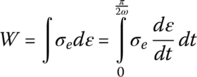
With σ e = E′ε 0 sin(ωt), the equation reduces to

From Eqs. (2.49) and (2.50), the loss factor η can be determined from
Hence, Eq. (2.51) defines the physical meaning of the loss factor as the ratio between the dissipated energy and stored energy. Also, Figure 2.12 shows the graphical representation and physical meaning of both the dissipated and stored energies.
2.5.3.2 Relationship Between Different Strains
Equations (2.45) and (2.46) can be rewritten as:
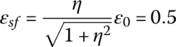
When the stress σ is set = 0, the corresponding strain ε sf can be obtained from:
or,
The σ − ε relationship of the upper branch of hysteresis characteristics can be expressed form Eq. (2.45) as:
The maximum stress is attained when:
![]() at ε = ε
maxσ
given by:
at ε = ε
maxσ
given by:
Figure 2.13 displays the graphical interpretation of the strains ε sf and ε maxσ .

Figure 2.13 Graphical representation of the strains ε sf and ε maxσ .
From Eqs. (2.53) and (2.55),
Hence, the loss factor can be computed as the ratio between the two strains ε sf and ε maxσ as measured from the hysteresis characteristics.
2.5.4 Storage Modulus
The storage modulus can be determined by considering the stress under a strain‐free condition σ stf . This value can be obtained by setting ε = 0 in Eq. (2.54), giving:
Once η and ε 0 are determined from Eqs. (2.56) and (2.53), then Eq. (2.57) can be used to compute the storage modulus E′.
Solution
The constitutive equation for the Poynting–Thomson model is:
For sinusoidal stress: σ = sin t, this equation reduces to:
This equation is integrated numerically, with respect to time, using MATLAB to extract the time history of the strain as function of the time history of the input stress. Then, the strain is plotted against the stress to yield the stress–strain characteristics shown in Figure 2.14.
- From Figure 2.14,

Then,

This yields ε 0 = 1.581.
Also, from Figure 2.14, σstf = ± ηE′ε 0 = ± 0.3148, or

-
From Table 2.10,

Then,

and

Hence, the two methods yield exactly the same results.

Figure 2.14 Stress–strain characteristics of a Poynting–Thomson model.
Solution
The storage modulus and the loss factor of the different VEM models, listed in Table 2.10, are plotted versus the frequency ω as shown in Figure 2.15. The plots are obtained for α = 1, β = 20, λ = 3, Es = 500, and E = 500.
The figure indicates clearly that all the three models are incapable of capturing the behavior of the Dyad606. However, the predictions of the Poynting–Thomson model qualitatively have the general trends but fail to quantitatively describe the behavior over a broad frequency range.
A combination of several Poynting–Thomson models is necessary to replicate the behavior of realistic VEMs.

Figure 2.15 Storage modulus and loss factor of different VEM models.
2.6 Fractional Derivative Models of Viscoelastic Materials
As indicated in Section 2.5, the simple classical models of VEMs cannot replicate the dynamic behavior of real VEMs. Other alternative models have been considered to overcome such serious limitations. Among these models are fractional derivative (FD) model (Bagley and Torvik 1983), Golla–Hughes–MacTavish (GHM) model (Golla and Hughes 1985), and the Augmented Temperature Field model (Lesieutre and Mingori 1990; Lesieutre et al. 1996).
2.6.1 Basic Building Block of Fractional Derivative Models
The basic concepts of fractional calculus are summarized in Appendix 2.B.
In this section, the basic building block of FD models is the “spring‐pot” that replaces the spring and dashpot elements used in the classical models. The spring‐pot element is employed to simplify, improve the applicability, and reduce the number of parameters used to model the complex behavior of viscoelastic polymers.
The spring‐pot element is a nonlinear FD element that has the following constitutive equation:
Note that the stress σ(t) applied to the element is dependent on the FD of order α of the strain ε(t) where α ranging between 0 and 1. When α = 0, the spring‐pot element reduces to a linear spring and when α = 1, the spring‐pot element becomes a linear dashpot (damper) as shown in Figure 2.16.

Figure 2.16 Representations of a spring‐pot, spring, and dashpot. (a) Spring‐pot, (b) spring, and (c) dashpot.
From Eq. (2.58), the storage and loss moduli of the spring‐pot can be determined as follows:

where ![]() and
and ![]() .
.
The relaxation modulus E(t) of the spring‐pot can be obtained by applying the inverse Fourier transform to Eq. (2.58) knowing that E(s) = E*/s, as indicated in Eq. (2.27b). This yields the following expressions:
Relaxation modulus

and
Creep compliance

2.6.2 Basic Fractional Derivative Models
The basic FD models presented in this section are the FD Maxwell, FD Kelvin–Voigt, and FD Poynting–Thomson models.
For example, consider the classical Maxwell model shown in Figure 2.17a is transformed to a FD Maxwell model shown in Figure 2.17b by replacing each component by a spring‐pot with different parameters.

Figure 2.17 Classical (a) and fractional derivative (b) Maxwell models.
For the FD model and using the equivalent spring‐pot Eq. (2.58), the strains ε 1 and ε 2 can be written as:
But as, ε = ε 1 + ε 2, then:
where ![]() ,
, ![]() , and α
1 ≥ α
2.
, and α
1 ≥ α
2.
Fourier‐transforming Eq. (2.63) gives:

Following the same approach adopted in Section 2.6.1, it can be easily shown that the relaxation modulus and creep compliance of the FD Maxwell model are given by:

Table 2.11 summarizes the complex moduli for the FD Maxwell, Kelvin–Voigt, and Zener models.
Table 2.11 Frequency domain characteristics of fractional derivative viscoelastic models.
| Parameter | Maxwell | Kelvin–Voigt | Zener |
| Model | 
|

|

|
| Storage modulus |  a
a
|
 b
b
|
a where ![]() ,
, ![]() , and α
1 ≥ α
2.
, and α
1 ≥ α
2.
b ![]() .
.
Solution
From Eq. (2.58), the complex modulus as predicted by the four‐parameter FD model can be obtained by using Eq. (2.B.10), to give:

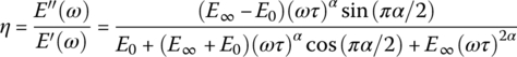
It can be easily shown that the storage and loss moduli of the four‐parameter FD model are given by:

and

Accordingly, the loss factor η is given by:
This yields a value of α that can be estimated from (see Problem 2.9):

Solution
The storage modulus and the loss factor of the FD and Poynting–Thomson VEM models are plotted versus the frequency ω as shown in Figure 2.18. The plots are obtained for the Poynting–Thomson model with α = 1, β = 20, λ = 3, and E s = 500 psi while the FD model is given by:

The figure indicates clearly that the four‐parameter FD model adequately replicates the physical behavior of Dyad 606 unlike the linear Poynting–Thomson model.

Figure 2.18 Storage modulus and loss factor of a fractional derivative and Poynting–Thomson models.
2.6.3 Other Common Fractional Derivative Models
In this section, some of the commonly used FD models are introduced. The main characteristics of these models are presented in the frequency ω domain as indicated in Table 2.12. These models vary in complexity by increasing the number of the included parameters from three (E ∞ , Δ, τ) as in the Debye model to five parameters (E ∞ , Δ, τ, α, and β) as in the Havriliak–Negami model (Pritz 2003, Ciambella et al. 2011).
Table 2.12 Frequency domain characteristics of fractional derivative viscoelastic models.
| Model | E * (ω) | Parameters |
| Debye |  a
a
|
3 |
| Cole–Coleb | 
|
4 |
| Cole–Davidson | 
|
4 |
| Havriliak–Negami | 
|
5 |
awhere Δ = (E 0 − E ∞)/E ∞ = relaxation strength, = relaxed elastic modulus, = unrelaxed elastic modulus.
bFriedrich and Braun (1992), Pritz (2003), and Ciambella et al. (2011).
Solution
According to the set parameters, the system equation reduces to:
or
where,

where A j + 1 = Grunwald coefficients.
Figure 2.20a,b displays the Grunwald coefficients and the time response of the spring‐mass system with a FD damper, respectively. It is evident, from Figure 2.20a, that the Grunwald coefficients vanish as the number of terms included in the summation of Eq. (2B.14) increases. This demonstrates clearly the “fading memory” characteristics of FDs. Figure 2.20b indicates that the system reaches, with an error of 3.14%, the desired reference command after 15 s.
Note that the approach adopted in Example 2.7 establishes the basis for time domain analysis of finite element models of structures treated with VEMs that are described by FD models.

Figure 2.19 A spring‐mass system with a fractional derivative damper.

Figure 2.20 Time response of a spring‐mass system with a fractional derivative damper.
2.7 Viscoelastic Versus Other Types of Damping Mechanisms
In this section, four important damping mechanisms are presented, including: viscous, hysteretic, structural, and friction damping in order to distinguish, compare, and relate their characteristics to those of viscoelastic damping materials.
Tables 2.13 and 2.14 summarize the main characteristics of these four damping mechanisms. Table 2.13 presents the physical representation of each mechanism, its mathematical model, force‐displacement characteristics, and a typical time response behavior.
Table 2.13 Characteristics of viscous, hysteretic, structural, and friction damping.
| Damping mechanism | Physical representation | Model | Force – displacement | Time response |
| Viscousa , b | 
|

|

|
|
| Hysteretica , b | 
|

|

|
|
| Structuralc , d | 
|

|

|
|
| Frictiona , b | 
|
|

|
Table 2.14 Energy dissipation and damping ratios of viscous, hysteretic, structural, and friction damping.
| Damping mechanism | Energy dissipation | Equivalent damping coefficient | Equivalent damping ratio |
| Viscous | D v = πcωX 2 | c v = c | |
| Hysteretic | D H = πkηX 2 | ||
| Structural | D S = 2kηX 2 | ||
| Friction | D F = 4F f X | 
|
|
| Viscoelastic | D VEM = πkηX 2 |
The energy dissipated per cycle by the different damping forces is calculated as follows:

where F d denotes the damping force as listed in the third column of Table 2.13.
The equivalent viscous damping coefficient, for any damping mechanism, is obtained by equating the energy dissipated by the ith mechanism to that of the viscous damping mechanism D v . Hence, the equivalent damping ratio of the ith mechanism is calculated as follows:
Equation (2.67) assumes that ζ
i
= c
i
/c
c
where ![]() is the critical damping coefficient for a single degree of freedom vibrating system.
is the critical damping coefficient for a single degree of freedom vibrating system.
Table 2.14 summarizes the energy dissipated per cycle, the equivalent viscous damping coefficients, and equivalent damping ratios of the different mechanisms in comparison with the corresponding values for viscoelastic materials.
2.8 Summary
This chapter has presented the classical models of VEMs. The merits and limitations of these models have been discussed both in the time and frequency domains. The energy dissipation characteristics of the VEMs have been presented with particular emphasis on the use of the unifying concept of the complex modulus. A brief description of the FD models has also been outlined to emphasize their utility and compactness. Measurement methods of the complex modulus of the VEMs will be presented in the next chapter, and extension of the classical models to more practical models that can be easily incorporated in the formulation of finite element method will be presented in Chapters 4–6.
References
- Bagley, R.L. and Torvik, P.J. (1983). Fractional calculus‐a different approach to the analysis of viscoelastically damped structures. AIAA Journal 21: 741–749.
- Beards, C. (1996). Structural Vibration: Analysis and Damping. London: Arnold.
- Christensen, R.M. (1982). Theory of Viscoelasticity: An Introduction, 2nde. New York: Academic Press Inc.
- Ciambella J., Paolone A., Vidoli S., “Dynamic Behavior of Viscoelastic Solids at Low Frequency: Fractional vs Exponential Relaxation”, 1–5. In Proceedings XX Congresso dell'Associazione Italiana di Meccanica Teorica e Applicata, Bologna 12–15 September 2011; F. Ubertini, E. Viola, S. de Miranda and G. Castellazzi (Eds.), ISBN 978‐88‐906340‐1‐7, 2011.
- Flugge, W. (1967). Viscoelasticity. Waltham, MA: Blaisdell Publishing Company.
- Friedrich, C. and Braun, H. (1992). Generalized Cole–Cole behavior and its rheological relevance. Rheologica Acta 31 (4): 309–322.
- Galucio, A.C., Deü, J.‐F., Mengué, S., and Dubois, F. (2006). An adaptation of the gear scheme for fractional derivatives. Computer Methods in Applied Mechanics and Engineering 195 (44–47): 6073–6085.
- Golla, D.F. and Hughes, P.C. (1985). Dynamics of viscolelastic structures – a time domain finite element formulation. ASME Journal of Applied Mechanics 52: 897–906.
- Gremaud G., “The Hysteretic Damping Mechanisms Related to Dislocation Motion”, Journal de Physique, Colloque C8, Supplement au N012, Tome 48, December 1987.
- Haddad, Y.M. (1995). Viscoelasticity of Engineering Materials. New York: Chapman & Hall.
- Heymans, N. (1996). Hierarchical models for viscoelasticity: dynamic behaviour in the linear range. Rheologica Acta 35 (5): 508–519.
- Iwan, W.D. (1964). An electric analog for systems containing Coulomb damping. Experimental Mechanics 4 (8): 232–236.
- Lakes, R. (1999). Viscoelastic Solids. Boca Raton, FL: CRC Press.
- Lakes, R. (2009). Viscoelastic Materials. Cambridge, UK: Cambridge University Press.
- Lesieutre, G.A., Bianchini, E., and Maiani, A. (1996). Finite element modeling of one‐dimensional viscoelastic structures using anelastic displacement fields. Journal of Guidance, Control, and Dynamics 19 (3): 520–527.
- Lesieutre, G.A. and Mingori, D.L. (1990). Finite element modeling of frequency‐dependent material damping using augmenting thermodynamic fields. Journal of Guidance, Control, and Dynamics 13 (6): 1040–1050.
- Muravskii, G.B. (2004). On frequency independent damping. Journal of Sound and Vibration 274: 653–668.
- Nashif, A., Jones, D., and Henderson, J. (1985). Vibration Damping. New York: Wiley.
- Nise, N.S. (2015). Control Systems Engineering, 7th Edn. Hoboken, NJ: Wiley.
- Oldham, K.B. and Spanier, J. (1974). An Introduction to the Fractional Calculus and Fractional Differential Equations. New York: Wiley.
- Padovan, J. (1987). Computational algorithms for FE formulations involving fractional operators. Computational Mechanics 2: 271–287.
- Podlubny, I. (1999). Fractional Differential Equations. San Diego, California: Academic Press.
- Pritz, T. (2003). Five‐parameter fractional derivative model for polymeric damping materials. Journal of Sound and Vibration 265: 935–952.
- Sun, C. and Lu, Y.P. (1995). Vibration Damping of Structural Elements. Englewood Cliffs, NJ: Prentice Hall.
- Rao, S.S. (2010). Mechanical Vibrations, 5the. New Jersey: Prentice Hall.
- Vondřejc, J. (2009). Constitutive models of linear viscoelasticity using Laplace transform. Czech Republic, Prague: Department of Mechanics, Faculty of Civil Engineering, Czech Technical University.
- Zener, C.M. (1948). Elasticity and Anelasticity of Metals. Chicago: University of Chicago Press.
2.A Initial and Final Value Theorems
The initial and final values of a function x(t) are given by the following theorems (Nise 2015):
- Initial value theorem:

- Final value theorem:

Proof
From the definition of the Laplace transform L:

Consider the following two extreme cases:
- when s → 0, this equation becomesthat is,


- when s → ∞, we havethat is,


2.B Fractional Calculus
2.B.1 Fractional Integration
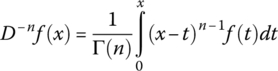
The fractional integral of a function f(x) with n‐folds is defined as:

Let

Then, integrating one more time gives:

Integrating another time gives:

After n integrations, yields the following expression, which is called “Reimann–Liouville Fractional Integral”:
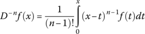
But, as Γ(n) = (n‐1)! = gamma function, then this equation reduces to:
2.B.2 Convolution Theorem
As the Laplace inverse of a product G(s) F(s) is given by the following convolution integral (Weber and Arfken 2003)1:
If
Then,
or
Equation (2.B.8) indicates that the fractional integration of f(x) is the convolution integral resulting from the inverse Laplace transformation of F(s) operated on by the n‐fold integral operator s −n .
Solution
With n = 1/2, Eq. (2.B.6) becomes:

which can be solved symbolically using MATLAB as follows:
2.B.3 Fractional Derivatives
Let m = p − l, then: D m f(x) = D p D −l f(x).
From Eq. (2.B.6),

If 0 < m < 1, then p = 1 or

Let n = 1 – l, then:

which is called the “Reimann–Liouville Fractional Derivative.”
Solution
With n = 1/2, Eq. (2.B.9) becomes:

which can be solved symbolically using MATLAB as follows:
2.B.4 Laplace Transform of Fractional Derivatives
Let n = 1 − l, then D n f(t) = D 1 D −l f(t).
Performing the Laplace transform, gives:

Integration by parts gives:

or
But as n = 1 − l, then:
2.B.5 Grunwald–Letnikov Definition of Fractional Derivatives
-
Integer Derivatives
Using the definition of integer derivatives in terms of a backward finite difference quotient, the following expressions can be extracted:


and

Hence, in general, the nth derivative can be written as:
Replacing Δt by t/N, then Eq. (2B.11) reduces to:
where the binomial coefficient
 for j > n.
 -
Fractional Derivatives
To extend Eq. (2B.12) to any fractional order derivative, the following extended definition of the binomial coefficient is used:

or
Substituting Eq. (2B.12) into Eq. (2B.13) gives:
where
 = Grunwald coefficients. These coefficients can be given also by the following recursive relationships:

and


Note that the Grunwald coefficients in Eq. (2B.15) decay to zero as the number of terms N increases. This feature describes the “fading memory” phenomenon which indicates that the behavior of the VEM is governed primarily by the recent time history rather than by the most remote history. Due to this property, it is possible to truncate higher order terms of summation in Eq. (2B.15) in order to simplify and speed the computational effort.
Other numerical algorithms to approach the FDs are summarized by Oldham and Spanier (1974), Padovan (1987), Podlubny (1999), and Galucio et al. (2006).
Solution
Figure 2.B.1 shows a comparison between the FDs predictions using the G–L and the R–L approaches. It is evident that close agreement is obtained between the two approaches. Note that the number of terms N used in the G–L summation is 12 000.

Figure 2.B.1 Comparison between the fractional derivative predictions using Grunwald–Letnikov (G–L) and the “Reimann–Liouville” (R–L) approaches.
Problems
- 2.1 Consider the Poynting–Thomson model of the VEM shown in Figure P2.1a. Derive the constitutive equation of the model that relates the applied stress σ to the resulting strain ε. Determine the creep behavior, during loading and unloading of the model according the cycle shown in Figure P2.1b, by solving the constitutive equation. Assume that σ = σ
0 and ε = σ
0/(E
p
+ E
s
) at t = 0 while σ = 0 and ε = ε
1 at t = t
1
.
Check the initial and final of the strain, during loading and unloading, using the initial and final value theorem (outlined in Appendix 2.A).

Figure P2.1 Poynting–Thomson model subjected to creep loading.
- 2.2 If a VEM is represented by the Poynting–Thomson model and is subjected to a step strain ε
0, show that the initial stress σ
0 experienced by the VEM is given by:

Use the initial value theorem.
- 2.3 Consider the three‐parameter Jeffery model of the VEM shown in Figure P2.2a. Derive the constitutive equation of the model that relates the applied stress σ to the resulting strain ε. Determine the creep behavior, during loading and unloading of the model according the cycle shown in Figure
P2.1b, by solving the constitutive equation. Assume that σ = σ
0 and ε = 0 at t = 0 while σ = 0 and ε = ε
1 at t = t
1
. Discuss the results.
Determine also the relaxation behavior when subjected to the strain loading shown in Figure P2.2b, by solving the constitutive equation. Assume that ε = ε 0 at t = 0. Discuss the results.

Figure P2.2 Jeffery model under relaxation loading.
- 2.4 Consider the three‐parameter models of a VEM shown in Figure P2.3.
Derive the constitutive equations of the models that relate the applied stress σ to the resulting strain ε. For sinusoidal excitations, at a frequency ω, such that σ = σ 0 e iωt and ε = ε 0 e iωt , use the derived constitutive equations to extract expressions for the complex modulus E, storage modulus E′, and loss factor η for each model [E = E′(1 + iη)].
If E s = 1, E p = 1, and c = 1, plot the effect of the frequency ω on the storage modulus E′and loss factor η for each model. Comment on the results.

Figure P2.3 Three‐parameter models (a) Poynting–Thomson model and (b) Zener model.
- 2.5 Derive the governing constitutive equations of Burgers model of a VEM, which is shown in Figure P2.4. Note that the model is combination between Maxwell and Kelvin–Voigt models.
For sinusoidal excitations at a frequency ω, such that σ = σ 0 e iωt and ε = ε 0 e iωt , extract expressions for the complex modulus E, storage modulus E′ and loss factor η for each model [E = E′(1 + iη)].
If E s = 1, E p = 1, and c = 1, plot the effect of the frequency ω on the storage modulus E′ and loss factor η for each model. Compare the results with those of the three‐parameter models of Problem 2.4.

Figure P2.4 Burgers model.
- 2.6 For the viscoelastic hysteresis loop shown in Figure P2.5 show that:
- the strain ε max = ε 0,
- the stress σ maxε = E′ε 0, and
- the loss factor η = σ stf /σ maxε .

Figure P2.5 The characteristics of viscoelastic hysteresis.
- 2.7 Show that the complex modulus of the Jeffery model of VEMs with an added inertia element I, as shown in Figure P2.6, is given by:


Figure P2.6 Jeffery model with added inertia.
- 2.8 Show that the complex modulus E
* of the hierarchical viscoelastic model of Figure P2.7, satisfies the following:

Show that this equation implies that:
 with λ = c
d
/E, that is, the hierarchical viscoelastic model is actually a FD model (Heymans 1996).
with λ = c
d
/E, that is, the hierarchical viscoelastic model is actually a FD model (Heymans 1996).
Figure P2.7 Hierarchical viscoelastic model.
- 2.9 The complex modulus as predicted by the four‐parameter FD model is given by:

Show that:
- the storage and loss moduli of the model are given by:

and

- the loss factor η is given by:

- the value of α that can be estimated from:

(Hint:
 , and
, and  )
) - the storage and loss moduli of the model are given by:
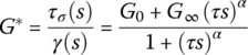
- 2.10 Determine the parameters of the following two fractional models:
 (Parameters are: G
0, G
∞, τ, α)
(Parameters are: G
0, G
∞, τ, α) (Parameters are: G
m
, τ, α)
(Parameters are: G
m
, τ, α)
that best fit the actual experimental behavior of Dyad606 VEM of Soundcoat operating at 38°C/100°F. Note that G, τ σ , and γ denote shear modulus, shear stress, and shear strain respectively. For these two models, derive the expressions for the:
- The storage modulus G′ and
- The loss factor η.
The storage modulus and loss factor of Dyad606 are given in the table here. Compare and comment on the results.
Frequency (Hz) 0.001 0.01 0.040 0.10 0.20 0.40 0.70 1.0 3.0 5.0 10 G′ (kpsi) 0.040 0.050 0.065 0.100 0.150 0.200 0.250 0.300 0.500 0.58 0.67 Loss Factor η 0.40 0.50 0.60 0.70 0.75 0.80 0.90 0.92 0.93 0.94 0.95 Frequency (Hz) 20 30 40 50 60 70 80 90 100 200 300 G′ (kpsi) 0.75 1.1 1.3 1.6 1.8 2 2.2 2.3 2.6 4 5.2 Loss Factor η 0.95 0.96 0.98 0.99 1. 1. 1. 1. 1. 0.99 0.95 Frequency (Hz) 400 500 600 700 800 900 1000 2000 3000 4000 5000 G′ (kpsi) 6.3 7.2 8.5 9.5 11 12 13 19 23 2.6 3 Loss Factor η 0.91 0.88 0.85 0.82 0.79 0.77 0.75 0.63 0.56 0.51 0.48 - 2.11 Show that the plots of loss modulus/E
s
versus the storage modulus/E
s
of the Maxwell, Kelvin–Voigt, and Poynting–Thomson models are as displayed in Figure P2.8. Note that these plots are called the “Nyquist diagrams” or “Cole–Cole” plots.

Figure P2.8 The Cole–Cole plots. - 2.12 Show that the plots of loss factor versus the storage modulus/E
s
of the Maxwell, Kelvin–Voigt, and Poynting–Thomson models are as displayed in Figure P2.9. Note that the plot is called the “Wicket” plot.

Figure P2.9 The “Wicket” plots. - 2.13 If the relaxation modulus of a VEM is given by:
E(t) = 1 + e −t in GPa, where t = time in seconds.
Determine its creep compliance J(t).
- 2.14 Show that the complex modulus E
* of the Ladder Viscoelastic Model in Figure P2.10, satisfies the following equation:

Also show this equation implies that:
 with λ = η/E
0.
with λ = η/E
0.
Figure P2.10 The ladder viscoelastic model.
- 2.15 Consider the dynamic system shown in Figure P2.11 that simulates the dynamics of VEMs. Derive the following:
- relationship between the force F and the net deflection (x
1
) in the following Laplace domain form:where K * = complex stiffness = K′(1 + i η) with K′ and η denoting the storage modulus and loss factor, respectively.

- storage modulus of the VEM K′ in terms of the frequency
- loss factor η of the VEM in terms of the frequency

Figure P2.11 Dynamic model of the viscoelastic material.
- relationship between the force F and the net deflection (x
1
) in the following Laplace domain form:
- 2.16 Show that the mechanical system with coulomb damping, which is displayed in Figure P2.12a, has the electrical analog circuit represented schematically in Figure P2.12b. Show also that the system has the hysteresis characteristics illustrated in Figure
P2.12c.
Relate the parameters of the mechanical elements of Figure P2.12a to those of their electrical analog components of Figure P2.12b. Note that q denotes the charge (Iwan, 1964).

Figure P2.12 Mechanical system with coulomb damping.