
5
Finite Element Modeling of Viscoelastic Damping by Modal Strain Energy Method
5.1 Introduction
The modal strain energy (MSE) method has been widely accepted as an effective and practical means for predicting the modal parameters of complex structures treated with viscoelastic damping treatments. The method is based on estimating the modal strain energies of the structure and the viscoelastic material (VEM) by using the undamped (real) mode shapes of the structure/VEM assembly instead of the exact damped (complex) mode shape. Such an approximation makes it easy to integrate the MSE with commercial finite element codes that generally do not use complex eigenvalue problem solvers. The theoretical basis of the original MSE method and several of its modified versions are presented. Application of the method to various types of viscoelastic damping treatments is discussed and compared with the predictions obtained by using the exact complex eigenvalue problem solvers and the Golla–Hughes–McTavish Model (GHM) approach discussed in Chapter 4.
5.2 Modal Strain Energy (MSE) Method
The MSE method was originally introduced by Kerwin and Ungar (1962) and then extended by Johnson and Kienholz (1982) as an approximate means for predicting the modal parameters of complex structures treated with viscoelastic damping treatments. The method is based on describing the viscoelastic material by the “complex modulus” approach and therefore, it is limited to frequency domain analysis. To account for the variation of the VEM properties with frequency, the MSE method becomes iterative in nature. In spite of these two limitations, the MSE method has been widely accepted because of its practicality and ease of integration with finite element models of structures treated with VEM without increasing the size of models as in the case of the GHM method (Golla and Hughes 1985).
The theory behind the MSE method starts by describing the dynamics of the structure/VEM system by the following finite element equation:
where {X} is the nodal deflection vector of the structure, [M] its mass matrix (real), and [K] is its stiffness matrix, which is complex to account for the VEM.
The stiffness matrix can be written as

where [Ke] and [Kv] are the stiffness matrices of the elastic structure and VEM, respectively. Also, ![]() and
and ![]() are the stiffness matrices corresponding to the storage and the dissipative components of the VEM stiffness, respectively. In Eq. (5.2), ηv denotes the loss factor of the VEM. Also, [KR] and [KI] denote the total elastic stiffness matrix of the structure/VEM and the dissipative stiffness matrix of the VEM. These matrices are given by
are the stiffness matrices corresponding to the storage and the dissipative components of the VEM stiffness, respectively. In Eq. (5.2), ηv denotes the loss factor of the VEM. Also, [KR] and [KI] denote the total elastic stiffness matrix of the structure/VEM and the dissipative stiffness matrix of the VEM. These matrices are given by
To cast the finite element model of Eq. (5.1) as an eigenvalue problem, the solution {X} can be written as
where ![]() and
and ![]() denote the eigenvector (mode shape) and eigenvalue (natural frequency) of the structure/VEM at mode n. These two quantities are complex and can be described as follows
denote the eigenvector (mode shape) and eigenvalue (natural frequency) of the structure/VEM at mode n. These two quantities are complex and can be described as follows
where ![]() and
and ![]() are the real and imaginary components of the eigenvector
are the real and imaginary components of the eigenvector ![]() . Also, ωn and ηn are the natural frequency and the loss factor of the nth mode.
. Also, ωn and ηn are the natural frequency and the loss factor of the nth mode.
Substituting Eq. (5.3) into Eq. (5.1) gives the following complex eigenvalue problem
Solution of this problem requires an iterative approach to account for the variation of both the storage and dissipative components of the stiffness matrix [K] with the frequency.
Substituting Eqs. (5.3) and (5.5) into Eq. (5.6) yields the following
Equating the real and imaginary parts on the two sides of Eq. (5.5), gives
and
Pre‐multiplying Eqs. (5.8) and (5.9) by ![]() gives
gives

and

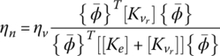
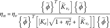
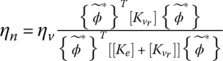
Dividing Eq. (5.11) by Eq. (5.10) and substituting for [KI] using Eq. (5.3) gives the modal loss factor ηn as follows

The MSE method simplifies Eq. (5.12) by replacing the exact damped (complex) mode shape ![]() by the undamped (real) mode shapes of the structure/VEM assembly
by the undamped (real) mode shapes of the structure/VEM assembly ![]() . Such simplification makes it easy to integrate the MSE with commercial finite element codes that generally do not use complex eigenvalue problem solvers.
. Such simplification makes it easy to integrate the MSE with commercial finite element codes that generally do not use complex eigenvalue problem solvers.
This yields the following expression

Physically, Eq. (5.13) means
that is, the loss factor of a structure/VEM assembly at the nth mode is equal to the loss factor of the VEM at the same frequency multiplied by the ratio of the MSE of the VEM to that of the structure/VEM assembly.
Implementation of MSE method is carried out according to the iterative scheme shown in Figure 5.1 in order to account for the variation of the VEM properties with frequency, the MSE method becomes in nature.
![Flowchart implementation of the MSE method, from input [M] and [Ke] matrices to iteration k = 1, to Input [Kνkr] and ηkν at frequencies ωkn, to for n = 1,..,N, to compute modal loss factor ηnk+1, etc.](http://images-20200215.ebookreading.net/1/4/4/9781118481929/9781118481929__active-and-passive__9781118481929__images__c05f001.gif)
Figure 5.1 Implementation of the MSE method.
Table 5.1 Comparison between the predictions of GHM and MSE methods for the rod/unconstrained VEM system.
| Method | GHM | MSE | ||
| Mode | Freq. (Hz) | Damping ratio | Freq. (Hz) | Damping ratio |
| 1 | 1103.50 | 0.002 42 | 1102.93 | 0.00 241 |
| 2 | 3869.42 | 0.001 57 | 3865.52 | 0.001 56 |
Table 5.2 Convergence of the iterative solution of the MSE method for the rod/unconstrained VEM system.
| Iteration | Mode 1 (Hz) | Mode 2 (Hz) | ζ1 | ζ2 |
| 1 | 1101.41 | 3847.69 | 0.000 17 | 0.000 036 |
| 2 | 1102.93 | 3865.51 | 0.002 40 | 0.001 56 |
| 3 | 1102.93 | 3865.52 | 0.002 41 | 0.001 56 |
Solution
Table 5.1 lists the natural frequencies and the corresponding modal damping ratios (MDRs) for the rod/unconstrained VEM system as obtained by the GHM, and the MSE methods. Table 5.2 lists the results of the iterative solution and its convergence when using the MSE method.
The displayed results suggest that the MSE method accurately predicts the modal parameters of the considered case. Furthermore, the MSE method converges after three iterations to the final modal parameters.
Table 5.3 Comparison between the predictions of the GHM and MSE methods for the rod/constrained VEM system.
| Method | GHM | MSE | ||
| Mode | Frequency (Hz) | Damping ratio | Frequency (Hz) | Damping ratio |
| 1 | 1113.06 | 0.0489 | 1103.81 | 0.0179 |
| 2 | 3757.96 | 0.0123 | 3740.42 | 0.0136 |
| 3 | 5191.08 | 0.0869 | 5071.87 | 0.0959 |
| 4 | 6417.20 | 0.0341 | 6395.56 | 0.0353 |
Solution
Table 5.3 lists the natural frequencies and the corresponding MDRs for the rod/constrained VEM system as obtained by the GHM and the MSE methods.
The displayed results show that the predictions of the modal parameters by the MSE are inaccurate for the considered case as compared to the predictions of the exact or the GHM methods. Such inaccuracy is attributed to the fact that approximating the exact (complex) eigenvectors by the undamped (real) eigenvectors is far from accurate because the loss factor is high in this case.
For this reason, several modified versions of the original MSE method have been developed to improve the estimates of the eigenvectors.
5.3 Modified Modal Strain Energy (MSE) Methods
Four modified versions of the original MSE method will be discussed in this section. These methods aim at developing improved eigenvectors to account for the imaginary component that has been neglected in the original MSE method. These methods range from heuristic methods, as the Weighted Stiffness Matrix (WSM) method (Hu et al. 1995) and the Weighted STorage Modulus method (WSTM) (Xu et al. 2002) to the more rigorous methods as the Improved Reduction System method (O'Callahan 1989; Scarpa et al. 2002) and the low frequency approximation (LFA) method (Scarpa et al. 2002).
5.3.1 Weighted Stiffness Matrix Method (WSM)
This method is based on substituting Eq. (5.5) into Eq. (5.5) to give
Equating the real part on both sides of this equation gives
Assume a vector ![]() to be defined such that:
to be defined such that:
Then, Eq. (5.15) reduces to
or
where [KM] = [KR] + β[KI] , β = a/b, and ![]() .
.
Eq. (5.16) represents a modified eigenvalue problem that has real eigenvalue ![]() and eigenvector
and eigenvector ![]() . Note that [KM] is a modified stiffness matrix that augments the elastic stiffness matrix [KR] with a weighted contribution of the imaginary component of the stiffness [KI]. The weighting parameter β is calculated from the following empirical formula proposed by Hu et al. (1995)
. Note that [KM] is a modified stiffness matrix that augments the elastic stiffness matrix [KR] with a weighted contribution of the imaginary component of the stiffness [KI]. The weighting parameter β is calculated from the following empirical formula proposed by Hu et al. (1995)

If β = 0, the modified eigenvalue problem reduces to that used in computing the real eigenvectors employed by the MSE method. If β ≠ 0, the modified eigenvalue problem attempts to heuristically account for the imaginary component of the stiffness in order to generate a better estimate ![]() of the real eigenvector. This estimate is used to compute the loss factor ηn of the nth mode as follows
of the real eigenvector. This estimate is used to compute the loss factor ηn of the nth mode as follows
5.3.2 Weighted Storage Modulus Method (WSTM)
In this method, the shear modulus of the VEM as described by
has a storage modulus G′ and loss factor ηv. Hence, to generate the real eigenvectors only G′ is used because it directly affects the real stiffness matrix ![]() of the VEM. However, a better estimate of the real eigenvectors can be obtained if the storage modulus is modified to account for the dissipative part. Xu et al. (2002) proposed to modify the storage modulus as follows
of the VEM. However, a better estimate of the real eigenvectors can be obtained if the storage modulus is modified to account for the dissipative part. Xu et al. (2002) proposed to modify the storage modulus as follows
In this manner, the modified storage modulus is the magnitude of the shear modulus that augments the storage modulus by the contribution of the loss modulus. Such a heuristic modification was motivated by the fact that increasing the storage modulus increases the natural frequencies and the observations that the natural frequencies increase with increasing the loss factor of the VEM as reported by Xu and Chen (2000) when using the exact complex eigenvalue problem solvers.
The loss factor of the structure/VEM system is then determined from
where ![]() is the elastic component of the stiffness matrix of the VEM as modified by the weighted storage modulus, that is,
is the elastic component of the stiffness matrix of the VEM as modified by the weighted storage modulus, that is, ![]() .
.
Also, ![]() is the eigenvector of the following eigenvalue problem:
is the eigenvector of the following eigenvalue problem:
5.3.3 Improved Reduction System Method (IRS)
This method is based on assuming the following modal transformation
where [Φ] is the eigenvector matrix for the undamped part of Eq. (5.1), that is,
such that
Also, in Eq. (5.22), {q} denotes the modal displacement vector, which is given by
But, for the damped system we have
Substituting Eqs. (5.22) and (5.24) into Eq. (5.25) gives
Pre‐multiplying Eq. (5.26) by [Φ]Tand using Eq. (5.23) gives
where ![]() .
.
Equating the real and imaginary parts on both sides of Eq. (5.23), gives the following matrix equation

or

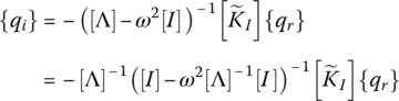
Using static condensation, the second row of Eq. (5.28) gives
and

Hence, the condensed system can be obtained by combining Eqs. (5.28) and (5.30) to yield the following
where
and
Solution of the eigenvalue problem given by Eq. (5.31) yields the eigenvalue ω and the eigenvector {qr}. The full complex eigenvector can be extracted as follows
This eigenvector can be used to compute the modal loss factor of the structure/VEM assembly as follows

5.3.4 Low Frequency Approximation Method (LFA)
This method is based on expanding the second row of Eq. (5.28) to give
or
For low frequencies, the Taylor series expansion of Eq. (5.29) in terms of ω is given by
Note that the first term of Eq. (5.35) is corresponding to the static condensation Eq. (5.29). In this manner, Eq. (5.35) includes the contribution of the inertia terms and accordingly presents a dynamic condensation of {qi) in terms of {qr}.
Expanding the first row of Eq. (5.28) gives:
Combining Eqs. (5.35) and (5.36) gives
Note that β is given by Eq. (5.17) as suggested by Hu et al. (1995).
Equation (5.37) presents a condensation equation with the transformation

Then, solving the original system given by Eq. (5.28) reduces to the following condensed system:
where
and
Solution of the eigenvalue problem given by Eq. (5.39) yields the eigenvalue ω and the eigenvector {qr}. The full complex eigenvector can be reconstructed as follows
This eigenvector can be used to compute the modal loss factor of the structure/VEM assembly as follows

Table 5.4 Comparison between the natural frequency predictions of the different modified MSE methods for the rod/constrained VEM system.
| Mode | GHM | MSE | Weighted stiffness | Weighted storage | IRS | LFA |
| 1 | 1113.06 | 1103.81 | 1105.26 | 1109.67 | 1111.89 | 1112.33 |
| 2 | 3757.96 | 3740.42 | 3740.81 | 3748.69 | 3746.69 | 3744.90 |
| 3 | 5191.08 | 5071.87 | 5072.19 | 5118.93 | 5059.11 | 5055.82 |
| 4 | 6417.20 | 6395.56 | 6395.32 | 6409.19 | 6391.55 | 6396.75 |
Table 5.5 Comparison between the damping ratio predictions of the different modified MSE methods for the rod/constrained VEM system.
| Mode | Exact | MSE | Weighted stiffness | Weighted storage | IRS | LFA |
| 1 | 0.0049 | 0.0179 | 0.0078 | 0.0049 | 0.0062 | 0.0346 |
| 2 | 0.0123 | 0.0136 | 0.0124 | 0.0124 | 0.0132 | 0.0135 |
| 3 | 0.0869 | 0.0959 | 0.0943 | 0.0942 | 0.0964 | 0.0952 |
| 4 | 0.0341 | 0.0353 | 0.0352 | 0.0352 | 0.0354 | 0.0361 |
Solution
Tables 5.4 and 5.5 list the natural frequencies and the corresponding MDRs for the rod/constrained VEM system as obtained by the exact eigenvalue problem solver of MATLAB, the MSE method, and four modified MSE methods.
It is clear that the four modified methods have improved the accuracy of the MSE. All the methods provide adequate predictions of the natural frequencies. Also, all the methods have predicted accurately the damping ratios except for the first mode with the exception of the LFA method.
5.4 Summary of Modal Strain Energy Methods
Table 5.6 summarizes the basic equations that are used to compute the modal loss factor using the conventional or the modified MSE methods. The table also lists the different forms of the eigenvectors needed to predict the modal loss factors for the considered MSE methods. Note that the MSE, WSM, and WSTM methods all use real eigenvectors while the IRS and LFA methods use imaginary eigenvectors.
Table 5.6 The basic equations used to determine the modal loss factor using the conventional or the modified MSE methods.
| Method | Modal loss factor | Eigenvectors | |
| MSE |  |
The real eigenvector { ϕn} is solution of: |
|
| MODIFIED MSE | Weighted Stiffness Matrix Method |  |
The real eigenvector where β = trace[KI]/trace[KR], |
| Weighted Storage Modulus Method |  |
The real eigenvector where |
|
| Improved Reduction System Method (IRS) |
The imaginary eigenvector { ϕ*} is given by: {ϕ*} = [Φ][[I] + i[S]]{qr} where with [Λ]and [Φ] are the eigenvalues and vectors of and {qr} = eigenvector of { [Kc] − ω2[Mc] } {qr} = 0 with [Mc] = [I] + [S]T[S], |
||
| Low Frequency Approximation Method (LFA) |
 |
The imaginary eigenvector where  β = trace[KI]/trace[KR], and {qr} = eigenvector of with |
|
5.5 Modal Strain Energy as a Metric for Design of Damping Treatments
The MSE, as described in Sections 5.1 through 5.4, serves as an important design metric for selecting the optimal design parameters (Lepoittevin and Kress 2009; Sainsbury and Masti 2007); location (Ro and Baz 2002); and topology of damping treatments (Ling et al. 2010).
Figure 5.2 summarizes the basic concept behind using the MSE as a design metric. For a given base structure (i.e., known [Ke] and [M]), an initial guess of the design parameters and/or topology (i.e., [Kv]), of the VEM is input to the MSE module to determine the modal loss factors ηn for the first N modes. These factors can be maximized for a particular mode or a group of critical modes by adjusting the design parameters and/or topology (i.e., [Kv]), of the VEM, in a rational manner, using available optimization tools such as the MATLAB Optimization Toolbox. This process is repeated until an optimal configuration of the VEM is attained while satisfying a set of design constraints.
![Block diagram of MSE as a design metric of VEM from input [Ke], [M] and [Kv] to modal strain energy, to output ηn, to optimization, to modify parameters or topology of VEM, back to [Kv].](http://images-20200215.ebookreading.net/1/4/4/9781118481929/9781118481929__active-and-passive__9781118481929__images__c05f002.gif)
Figure 5.2 MSE as a design metric of VEM.
In this section, the MSE will be utilized in selecting the optimal thickness of unconstrained damping layers which are used to treat rods undergoing longitudinal vibrations.
In order to illustrate the utility of the MSE as a design metric, consider the following example:

Figure 5.3 Finite element model of a rod treated with unconstrained VEM.

Figure 5.4 Optimal thickness distribution of VEM for constraint set 1 and objective function F1.

Figure 5.5 Optimal thickness distribution of VEM for constraint set 2 and objective function F1.

Figure 5.6 Optimal thickness distribution of VEM for constraint set 1 and objective function F2.

Figure 5.7 Optimal thickness distribution of VEM for constraint set 2 and objective function F2.

Figure 5.8 Time response of optimal damping treatment designs based on objective function F2. (a) Constraint set 1 and (b) constraint set 2.
Solution
The design problem is formulated mathematically as follows:

In this optimum design problem, the objective function is written as the ratio of the sum of the modal loss factor for the first five modes to the total weight of the treatment. In this manner, maximizing F will simultaneously ensure maximizing the modal loss factor and minimizing the total weight. The constraints imposed on the design problem ensure that all the design variables tvi are positive and each is bounded from below and from above by tvmin and tvmax, respectively.
Note that the lower bound is selected to ensure adequate damping and avoid reaching the unrealistic trivial solution where all the design variables tvi vanish, which makes the mass of the treatment minimum (= zero) and the objective function maximum (= ∞). However, the upper bound is selected to avoid an impractically thick VEM.
Consider the following objective functions:
- F1 = sum of the modal loss factor for the first five modes

Two sets of constraints are imposed:
Set 1: tvmin = 0.001 and tvmax = 0.01 m
Let the initial guess of the thickness distribution is [tv1, tv2, …, tv5] = [0.005 0.005 0.005 0.005 0.005]. The MATLAB solution of the optimization problem using the “fmincon” subroutine of the Optimization Toolbox gives optimal thicknesses = [0.01 0.01 0.01 0.01 0.01] as displayed in Figure 5.4. The corresponding value of the objective function F1 = 0.002 043.
Set 2: tvmin = 0.001 and tvmax = 0.025 m
If the initial guess of the thickness distribution is maintained at [tv1, tv2, …, tv5] = [0.005 0.005 0.005 0.005 0.005]. The MATLAB solution of the optimization problem using the “fmincon” subroutine of the Optimization Toolbox gives optimal thicknesses = [0.025 0.025 0.025 0.025 0.025] as displayed in Figure 5.5. The corresponding value of the objective function F1 = 0.005 44.
In both cases, the optimum is attained when the thickness of each element attains the allowable upper bound in order to maximize the sum of the modal loss factor for the first five modes. Accordingly, the optimization algorithm pushes the VEM thickness to its maximum limit without any regard to the weight.
- F2 = sum of the modal loss factors/total weight

In this case, the objective function F2 puts a penalty on the weight of the VEM.
Two sets of constraints are imposed:
Set 1: tvmin = 0.001 and tvmax = 0.025 m
If the initial guess of the thickness distribution is [tv1, tv2, …, tv5] = [0.005 0.005 0.005 0.005 0.005]. MATLAB Optimization Toolbox gives optimal thicknesses = [0.025 0.001 0.001 0.001 0.001] as displayed in Figure 5.6. The corresponding value of the objective function F2 = 0.002 28.
Set 2: tvmin = 0.01 and tvmax = 0.025 m
If the initial guess of the thickness distribution is [tv1, tv2, …, tv5] = [0.01 0.01 0.01 0.01 0.01]. MATLAB Optimization Toolbox gives optimal thicknesses = [0.025 0.012 0.01 0.01 0.01] as displayed in Figure 5.7. The corresponding value of the objective function F2 = 0.001 73.
Figure 5.8a,b show the time response of the rod when treated with the optimal damping treatments corresponding to constraint sets 1 and 2, which are imposed on objective function F2. The rod in both cases is subjected to a unit impulse at its free end.
It is important to note that although the optimal objective function for the first set of constraints is F2 = 0.002 28 and that for the second set is F2 = 0.001 73, the vibration damping characteristics for the second set is better than the first. This is attributed to the fact that the weight of the VEM for the second set is 2.39 times that of the first set. Hence, the sum of the modal loss factors for the second set is almost twice that of the first set. Accordingly, more damping is achieved with the second set of constraints in spite of the lower value of the objective function.
5.6 Perforated Damping Treatments
5.6.1 Overview
Engineered Damping Treatments (EDTs) that have high damping characteristics per unit volume are presented in this section. The EDTs under consideration consist of cellular viscoelastic damping matrices with optimally selected cell configuration, size, and distribution. These perforated EDTs are intended to replace conventional viscoelastic damping treatments to improve their damping characteristics and reduce their weight at the same time. Examples of such perforated EDTs are shown in Figure 5.9. The number, shape, and spacing of the perforations are critical to the effective damping characteristics of the treatment and to the minimization of its weight. Figure 5.9a–c shows a conventional damping treatment, treatment with square holes that has a positive Poisson's ratio, and treatment with reentrant hexagon holes that has a negative Poisson's ratio.

Figure 5.9 Perforated damping treatment. (a) Conventional treatment. (b) Treatment with square holes. (c) Treatment with reentrant hexagonal holes.
The cellular topologies of the EDTs are modeled using the finite element method in an attempt to determine the optimal topologies that maximize the strain energy, maximize the damping characteristics, and minimize the total weight. The damping characteristics of the manufactured EDTs are evaluated and compared with the corresponding characteristics obtained by conventional solid damping treatments in order to emphasize the importance of using optimally configured damping treatment to achieve high damping characteristics.
5.6.2 Finite Element Modeling
Consider the configuration shown in Figure 5.10. It consists of a base plate covered from one side with a layer of VEM. The base plate is isotropic and linearly elastic with density, elasticity modulus, and Poisson's ratio of ρp, Ep, vp, respectively. The VEM layer properties are denoted by ρv, Ev, vv where the complex elasticity modulus Ev = E0(1 + jη) is used to describe the viscoelastic properties of the layer. The viscoelastic layer is conventionally solid with constant thickness or it can have a variable thickness to maximize the damping behavior.

Figure 5.10 Plate treated with unconstrained damping treatment. (a) Plate/VEM element. (b) Local coordinates and node labeling.
Figure 5.10b shows a finite element of this composite. The element is a four‐noded rectangular element with dimensions 2a × 2b while the thicknesses of the base layer and the treatment are hp and hv, respectively. The plate element is aligned to the x–y‐plane. The displacement components of the base plate are u, v, and w in the x, y, and z directions. Also, θx and θy are the rotational components about the x and y directions. The displacement vector u of the base plate is given by: u = {u v w θx θy}T. Accordingly, each node has five degrees of freedom corresponding to the five displacement components. Furthermore, the base plate is assumed to be thin and hence the strain components εxz, εyz, and εzz vanish. According to this assumption, the rotation degrees of freedom can be expressed in terms of the gradients of the lateral deflection such that
The other strain components are


Within the finite element, the displacement vector is approximated as

where q = {p1 p2 p3 p4}T= nodal deflection vector of the four nodes and N represents the appropriate shape function. Using bilinear interpolation functions ϕ1 for the variation of in‐plane displacement components (u and v) and bi‐cubic interpolation functions ϕ2 for the variation of lateral displacement and rotation components (w, θx, or θy) such that:
and
Then, C is a 5 × 20 matrix that includes the basis functions for all the five variables, that is:

Hence, the shape function N is also a 5 × 20 matrix, which can be expressed as:

For the VEM layer, the five degrees of freedom are as follows:

where T is the transformation matrix relating the degrees of freedom of the VEM to those of the base plate.
5.6.2.1 Element Energies
The total kinetic energy T of the composite plate is the summation of the kinetic energies of the plate and VEM, which are denoted by Tp and Tv respectively. T is given by:
For the ith layer in the eth element:

Similarly, the total potential energy of the composite plate is the summation of the plate and VEM elastic energies.
For the ith layer in the eth element:

In Eq. (5.55), the stress–strain relationship is given by:

The equation of motion for plate/VEM system can then be reduced to:
where KR is the real part of global stiffness matrix and KI is the imaginary part of global stiffness matrix. Therefore, the nth MDR can be written:

where ϕn is the nth eigenvector.

Figure 5.11 Three types of damping treatment. (a) Conventional treatment. (b) Treatment with square holes. (c) Treatment with reentrant hexagonal holes.

Figure 5.12 Finite element models of the three viscoelastic treatments. (a) Conventional treatment. (b) Treatment with square holes. (c) Treatment with reentrant hexagonal holes.
Table 5.7 Comparison between the natural frequencies, modal damping ratios (MDR), modal strain energy (MSE) in VEM and modal strain energy MSE per unit volume for the different viscoelastic treatments.
| Mode number | Natural frequencies (Hz) | ||
| Conventional | Squares | Reentrant hexagons | |
| 1 | 24 | 23 | 23 |
| 2 | 52 | 50 | 51 |
| 3 | 114 | 113 | 113 |
| 4 | 145 | 143 | 143 |
| Mode number | MDR (%) | ||
| Conventional | Squares | Reentrant hexagons | |
| 1 | 0.006015 | 0.005551 | 0.005734 |
| 2 | 0.006070 | 0.005350 | 0.005627 |
| 3 | 0.008950 | 0.007724 | 0.008188 |
| 4 | 0.009249 | 0.007556 | 0.008196 |
| Mode Number | MSE in VEM (mJ cycle−1) | ||
| Conventional | Squares | Reentrant hexagons | |
| 1 | 0.48 | 0.45 | 0.46 |
| 2 | 1.03 | 0.99 | 1.01 |
| 3 | 2.26 | 2.22 | 2.24 |
| 4 | 2.86 | 2.82 | 2.83 |
| Mode Number | MSE in VEM/Treatment Volume (GJ m−3) | ||
| Conventional | Squares | Reentrant hexagons | |
| 1 | 4.74 | 5.54 | 5.33 |
| 2 | 11.02 | 12.19 | 11.71 |
| 3 | 22.32 | 27.32 | 25.97 |
| 4 | 28.25 | 34.71 | 32.81 |
| Average | 16.58 | 19.94 | 18.96 |
| %Gain | 0 | 20.26% | 14.32% |
Solution
Figure 5.12 displays the finite element models of the considered three damping treatment configurations.
The results in Table 5.7 indicate that the natural frequencies and MSE in the VEM of the three treatments are nearly the same. However, the MDRs of the conventional treatment are slightly higher than those of treatments with square or reentrant hexagon holes. But, the results reveal that the treatments with square perforations has the highest MSE in VEM (i.e. dissipated energy) per unit volume of VEM followed by the treatments with reentrant hexagon holes and then the conventional treatments came last. The percentage gains in the dissipated energy relative to the conventional treatments are 20.26 and 14.32% for treatments with square holes and treatments with reentrant hexagon holes, respectively.
5.6.2.2 Topology Optimization of Unconstrained Layer Damping
The energy dissipation of plate/constrained layer damping comes from the shearing deformation in VEM layer, it is reasonable to consider the MDR or modal loss factor of damping structures as the objective function of topology optimization (El‐Sabbagh and Baz 2014). Therefore, the objective function is written:

where f denotes the objective function of the optimization problem in present study. m represents the number of the considered MDR. Define the relative density of each VEM element as the design variable vector:
In addition, the constraint is considered to limit the consumption of VEM, the volume fraction is considered. The optimization problem is formulated as follows:

where N is the number of elements, Φj is the eigenvector, M and Kare the global mass and stiffness matrices, and V/V0 = α = volume fraction of viscoelastic material on the plate.
According to the Solid Isotropic Material with Penalization (SIMP) topology optimization method, the element mass and stiffness matrices can be expressed as the product of variables density and the entity element mass and stiffness matrices. The penalty factors p, q; p, q ≥ 1 are put in to accelerate the convergence of iteration results, that is:
where ρe is variable density of each VEM element; it is a relative quantity and 0 ≤ ρe ≤ 1. Note that if, ρe = 0 then there is no VEM treatment for this element or equivalently, the thickness of the VEM is equal to zero. Similarly, if ρe = 1, then the thickness of VEM in this element is equal to the assigned thickness. Also, ![]() ,
, ![]() are the mass and stiffness matrices of VEM element. Keep the base plate and constrained layer unchanged, the global mass, and stiffness matrices can be calculated as follows:
are the mass and stiffness matrices of VEM element. Keep the base plate and constrained layer unchanged, the global mass, and stiffness matrices can be calculated as follows:


where p and q are penalty factors, p = 1, q = 3. The layout of VEM on the plate can be determined by searching the optimal relative density of each VEM element. In order to solve the presented optimum problem, Method of Moving Asymptote (MMA) method is employed.
5.6.2.3 Sensitivity Analysis
According to MSE method, approximate expressions of the ith MDR can be obtained. The equation of motion for plate/VEM system is given:
where KR is the real part of global stiffness matrix, KI is the image part of global stiffness matrix. Therefore, the nth MDR can be written:

where ϕr is the nth eigenvector, the derivatives of Eq. (5.66) to design variables are:

The derivatives of the stiffness matrix are obtained by solving the following sensitivity equations:

and

when p = 1, q = 3, the derivative of MDR can be expressed as:

The dynamic constraint function is
The derivative of the dynamic constraint function is calculated as follows:

and

When p = 1, q = 3, the sensitivity of constrained functions become:

Figure 5.13 presents the flow chart of the topology optimization using the MMAs proposed by Svanberg (1987, 2002) to determine the optimal distribution of damping material over structures. It is noted that the computation time is mainly determined by building/solving the finite element model with the complex stiffness matrices and using the MMA approach.

Figure 5.13 Block diagram for the MMA optimization procedures.

Figure 5.14 Initial configuration of a plate treated with an unconstrained VEM damping treatment.

Figure 5.15 Optimal topology of a VEM treatment of a cantilevered plate with volume ratio of 0.25. (a) Modal damping ratios. (b) Optimal topology.

Figure 5.16 Optimal topology of a VEM treatment of a cantilevered plate with volume ratio of 0.5. (a) Modal damping ratios. (b) Optimal topology.

Figure 5.17 Optimal topology of a VEM treatment of a cantilevered plate with volume ratio of 0.75. (a) Modal damping ratios. (b) Optimal topology.
Solution
A finite element code is developed to describe the dynamics of a plate treated with VEM as outlined in Section 5.6.2. The finite element model is used to extract the strain energy in order serve as a quantitative measure for computing the MDR. Then, the MMA topology optimization method outlined in Sections 5.6.2.2 and 5.6.2.3 is employed to determine the optimal topology of surface damping treatments.
Figures 5.15–5.17 present the optimal topologies of the VEM for volume ratios of 0.25, 0.5, and 0.75 in order to maximize the MDR of the first mode. The figures display also the effect of optimization iteration number on the MDRs of the first four modes.
The figures indicate that the optimum MDRs for the first mode attain their peak values nearly after 2000 iterations. These optimal damping ratios are 0.0002, 0.00026, and 0.00024 for volume ratios of 0.25, 0.5, and 0.75 respectively. These damping ratios as well as those for higher order modes increase with increasing volume ratios. The figures indicate also that the obtained optimal topologies tend to concentrate the VEM near the fixed end of the plate with additional treatments placed at the mid‐section of the plate near its free end.
Furthermore, it is observed that the MMA algorithm converges faster as the volume ratio of the VEM is increased.

Figure 5.18 Optimal topology of a VEM treatment of a simply supported plate with volume ratio of 0.25. (a) Modal damping ratios. (b) Optimal topology.
Figure 5.19 Optimal topology of a VEM treatment of a simply supported plate with volume ratio of 0.50. (a) Modal damping ratios. (b) Optimal topology.
Figure 5.20 Optimal topology of a VEM treatment of a simply supported plate with volume ratio of 0.75. (a) Modal damping ratios. (b) Optimal topology.
Solution
The approach adopted in solving Problem 5.6 is used. However, the simply supported boundary condition is imposed on the finite element model. Solving the topology optimization problem of the VEM, for volume ratios of 0.25, 0.5, and 0.75, yields the optimal topologies shown in Figures 5.18–5.20, respectively. The figures display also the effect of optimization iteration number on the MDRs of the first four modes.
The figures indicate that the optimum MDRs for the first mode attain their peak values nearly after 2000 iterations. These optimal damping ratios are 0.00032, 0.00042, and 0.00044 for volume ratios of 0.25, 0.5, and 0.75 respectively. These damping ratios as well as those for higher order modes increase with increasing volume ratios. The figures indicate also that the obtained optimal topologies tend to concentrate the VEM near the fixed end of the plate with additional treatments placed at the mid‐section of the plate near its free end.
5.7 Summary
This chapter has presented the MSE method with its original and modified forms. The theories behind the MSE method and its modifications are presented. Numerical examples are given to quantify the accuracy of the different method in predicting the modal parameters of rods treated with VEM.
The MSE has also been shown to serve as an important design metric for selecting the optimal design parameters and/or determining the optimal topologies of damping treatments based on rational design objectives.
References
- Curà, F., Mura, A., and Scarpa, F. (2011). Modal strain energy based methods for the analysis of complex patterned free layer damped plates. Journal of Vibration and Control 18 (9): 1291–1302.
- El‐Sabbagh, A. and Baz, A. (2014). Topology optimization of unconstrained damping treatments for plates. Engineering Optimization 46 (9): 1153–1168.
- Golla, D.F. and Hughes, P.C. (1985). Dynamics of viscolelastic structures – a time domain finite element formulation. ASME Journal of Applied Mechanics 52: 897–600.
- Hu, B.‐G., Dokainish, M.A., and Mansour, W.M. (1995). Modified MSE method for viscoelastic systems: a weighted stiffness matrix approach. Journal of Vibration and Acoustics, Transactions of the ASME 117 (2): 226–231.
- Johnson, C.D. and Kienholz, D.A. (1982). Finite element prediction of damping in structures with constrained viscoelastic layers. AIAA Journal 20: 1284–1290.
- Kerwin, E.M. and Ungar, E.E. (1962). Loss factors of viscoelastic systems in terms of energy concepts. Journal of Acoustical Society of America 34: 954–957.
- Lepoittevin, G. and Kress, G. (2009). Optimization of segmented constrained layer damping with mathematical programming using strain energy analysis and modal data. Materials & Design 31 (1): 14–24.
- Ling, Z., Ronglu, X., Yi, W., and El‐Sabbagh, A. (2010). Topology optimization of constrained layer damping on plates using method of moving asymptote (MMA) approach. Shock and Vibration doi: 10.3233/SAV‐2010‐0583.
- O'Callahan J., “A procedure for an improved reduced system”, Proceedings of the International Modal Analysis Conference (IMAC), pp. 17–21, 1989.
- Ro, J. and Baz, A. (2002). Optimal placement and control of active constrained layer damping using modal strain energy approach. Journal of Vibration and Control 8 (8): 861–876.
- Sainsbury, M.G. and Masti, R.S. (2007). Vibration damping of cylindrical shells using strain‐energy‐based distribution of an add‐on viscoelastic treatment. Finite Elements in Analysis and Design 43 (3): 175–192.
- Scarpa F., Landi F. P., Rongong J. A., DeWitt L., and Tomlinson G., “Improving the MSE method for viscoelastic damped structures”, Proceedings of SPIE – The International Society for Optical Engineering, Vol. 4697, pp. 25–34, 2002.
- Svanberg, K. (1987). The method of moving asymptotes: a new method for structural optimization. International Journal for Numerical Methods in Engineering 24: 359–373.
- Svanberg, K. (2002). A class of globally convergent optimization methods based on conservative convex separable approximations. SIAM Journal on Optimization 12 (2): 555–573.
- Xu Y. and Chen D., “Finite element modeling for the flexural vibration of damped sandwich beams considering complex modulus of the adhesive layer”, Proceedings of SPIE – Damping and Isolation, Vol. 3989, pp. 121–129, 2000.
- Xu Y., Liu Y., and Wang B., “Revised modal strain energy method for finite element analysis of viscoelastic damping treated structures”, Proceedings of SPIE – The International Society for Optical Engineering, Vol. 4697, pp. 35–42, 2002.
Problems
- 5.1 Consider the fixed‐free rods shown in Figure P5.1. Determine the natural frequencies and the damping ratios of the two rod/VEM systems using the MSE method and its four modified versions discussed in Section 5.3.
Assume the dimensions and the material properties of the two systems are as given in Example 4.3.
Assume also that the two systems are modeled using three finite elements.

Figure P5.1 Complete and segmented UCLD treatments. (a) Complete UCLD. (b) Segmented UCLD.
- 5.2 Consider the fixed‐free rods shown in Figure P5.2. Determine the natural frequencies and the damping ratios of the two rod/VEM systems using the MSE method and its four modified versions discussed in Section 5.3.
Assume the dimensions and the material properties of the two systems are as given in Example 4.4.
Assume also that the two systems are modeled using three finite elements.

Figure P5.2 Complete and segmented CLD treatments. (a) Complete CLD. (b) Segmented CLD.
- 5.3 Consider the dynamical system shown in Figure P5.3a. The mass m is supported on two springs. One of these springs is an elastic spring with real stiffness k1 while the third spring is viscoelastic with complex stiffness
 where η is the loss factor of the VEM. Show that:
- the equivalent system shown in Figure P5.3b has:

where

- the loss factor ηMSE of this system, as calculated by using the MSE concept, is given by:


Figure P5.3 Mass supported on a VEM and a spring. (a) Original system. (b) Equivalent system.
- 5.4 Consider the dynamical system shown in Figure P5.4a. The mass m is supported on three springs. Two are elastic springs with real stiffness k1 and k3, respectively, while the third spring is viscoelastic with complex stiffness
 where η is the loss factor of the VEM. Show:
- that this system is equivalent to the system shown in Figure P5.4b such that:
where
 , with K21 = k2/k1 and K23 = k2/k3.
- that the loss factor ηMSE of this system as calculated by using the MSE concept is given by:

- that the error between the exact loss factor ηs and that ηMSE estimated by MSE is:

That is, MSE over estimates the exact loss factor.

Figure P5.4 Mass supported on a VEM and two springs (a) Original system. (b) Equivalent system.
- 5.5 Consider the dynamical system shown in Figure P5.5. The vibration of the primary system (m1–k1) is controlled by the secondary system (i.e., a dynamic damper system). Assume that m1 = m2 = 1kg, k1 = 1 N m−1, and
 , then:
- Derive the equations of motion of the system and cast in the following form:

where [M] = mass matrix, [KR] = real stiffness matrix, [KI] = imaginary stiffness matrix, and
- Determine the MDRs of the two modes of vibration of the system using the Original Modal Strain Method (MSE).

Figure P5.5 Primary system with a dynamic damper.
- 5.6 Consider the dynamical system shown in Figure P5.6. The mass m is supported on four springs. Three of these springs is an elastic spring with real stiffness k1 while the fourth spring is viscoelastic with complex stiffness
 where η is the loss factor of the VEM. Determine the loss factor of the system using:
- the equivalent system shown in Figure P5.6 such that K* = KR(1 + ηsi)
- the MSE concept such that the loss factor = ηMSE
- Compare the results obtained in a and b.

Figure P5.6 Mass supported on a VEM and three springs (a) Original system. (b) Equivalent system.
- 5.7 Consider the fixed‐free rod/VEM system shown in Figure P5.7. The rod is made of aluminum with width of 0.025 m, thickness of 0.025 m, and length of 1 m. The VEM has a width of 0.025 m, thickness = tv m, and density 1100 kg m−3. The VEM is constrained by an aluminum constraining layer that is 0.025 m wide and 0.0025 m thick. Using the GHM modeling approach of the VEM with one mini‐oscillator (E0 = 15.3MPa, α1 = 39, ζ1 = 1, ω1 = 19, 058rad/s), determine:
- the optimum thickness tv of the VEM that maximizes the sum of the MDRs for the two modes of vibration the end/VEM (use the MSE as a design criterion).
- the optimum thickness tv of the VEM that maximizes the sum of the MDRs for the two modes of vibration the end/VEM per unit weight of the VEM treatment (use the MSE as a design criterion).
Assume that the system is modeled by a two element finite element model and that tv is constrained such that: 0.005 ≤ tv ≤ 0.05 m.
Comment on the optimum results obtained in items a and b.

Figure P5.7 A fixed‐free rod treated with a constrained VEM layer.
- 5.8 Consider the cantilever beam/passive constrained layer damping (PCLD) system shown as Figure P5.8. The main physical and geometrical parameters of the base beam, the viscoelastic layer and constrained layer are listed in Table P5.1. The beam is made of aluminum and is mounted in a cantilever configuration. The beam is treated with segmented arrangements of viscoelastic material that are constrained by an aluminum layer as shown in Figure P5.8 (Curà et al. 2011).
Determine the sum of the MDRs of the beam/stripped VEM assembly for the first four modes of vibration.
Determine such sum for three arrangements shown in Figure P5.8.

Figure P5.8 Cantilever beam treated with segmented PCLD treatments (a) PCLD‐Plain. (b) PCLD‐Plain‐PCLD‐Plain. (c) PCLD‐Plain‐PCLD‐Plain PCLD‐Plain‐PCLD‐Plain.
Table P5.1 Physical and geometrical parameters of a plate/PCLD system.
Layer Length (m) Width (m) Thickness (mm) Density (kg m−3) Modulus (MPa) Base Plate 0.32 0.125 0.50 2700 7100a Viscoelastic stripped 0.125 0.50 1140 20b Constraining Layer stripped 0.125 0.25 2700 7100a a Young's modulus.
b Shear modulus, η = 0.5.
- 5.9 Consider the cantilever plate/PCLD system shown as Figure P5.9. The main physical and geometrical parameters of the base plate, the viscoelastic layer and constrained layer are listed in Table P5.2. The plate is made of aluminum and is mounted in a cantilever configuration. The plate is treated with viscoelastic material, which is constrained by a continuous Polyvinylidene Fluoride (PVDF) piezoelectric layer as shown in Figure P5.9.
Using the topology optimization approach, determine the optimal distribution of the VEM over the plate surface in order to maximize the sum of the MDRs of the plate/VEM assembly for the first four modes of vibration.
Determine such optimal topologies for volume fractions of the VEM of 0.2, 0.4, 0.6, and 0.8 (Ling et al. 2010).

Figure P5.9 A cantilever plate treated with PCLD treatments (a) Plate with PCLD treatment. (b) VEM treatment with optimally placed voids.
- 5.10 Using the topology optimization approach, determine the optimal distribution of the VEM over the plate surface of Problem 5.9 when the plate is anchored in a simply‐supported configuration as shown in Figure P5.10. The topology optimization aims at maximizing the sum of the MDRs of the plate/VEM assembly for the first four modes of vibration.
Determine such optimal topologies for volume fractions of the VEM of 0.2, 0.4, 0.6, and 0.8.

Figure P5.10 A simply supported plate treated with PCLD treatment.