
10
Vibration Control with Periodic Structures
10.1 Introduction
Periodic structures, whether passive or active, are structures that consist of identical substructures, or cells, connected in an identical manner as shown in Figures 10.1 and 10.2. Because of their periodic nature, these structures exhibit unique dynamic characteristics that make them act as mechanical filters for wave propagation. As a result, waves can propagate along the periodic structures only within specific frequency bands called the “pass bands” and wave propagation is completely blocked within other frequency bands called the “stop bands” as shown in Figure 10.3a. The spectral width and location of these bands are fixed for passive periodic structures, and are tunable in response to the structural vibration for active periodic structures as indicated in Figure 10.3b (Baz 2001).

Figure 10.1 Typical examples of passive periodic structures: (a) with geometrical discontinuity and (b) with material discontinuity.

Figure 10.2 Typical examples of active periodic structures: (a) with active piezoelectric patches and (b) with active shape memory inserts.

Figure 10.3 Pass and stop bands of passive and active periodic structures. (a) Passive with fixed bands and (b) active with tunable bands.
The theory of periodic structures was originally developed for solid state applications (Brillouin 1946) and extended, in the early 1970s, to the design of mechanical structures (Mead 1970; Cremer et al. 1973). Since then, the theory has been extensively applied to a wide variety of structures such as spring‐mass systems (Faulkner and Hong 1985); periodic rods (Ruzzene and Baz 2000); periodic beams (Mead 1970; Mead and Markus 1983; Roy and Plunkett 1986; Faulkner and Hong 1985); stiffened plates (Sen Gupta 1970; Mead 1971, 1986; Mead and Yaman 1991); ribbed shells (Mead and Bardell 1987; Ruzzene and Baz 2001); and space structures.
Apart from their unique filtering characteristics, the ability of periodic structures to transmit waves from one location to another within the pass bands can be greatly reduced when the ideal periodicity is disrupted or disordered (Hodges 1982; Hodges and Woodhouse 1983). This results in the well‐known phenomenon of “localization,” whereby the effects of an external disturbance are localized at (or confined to) the structural zone surrounding it.
In the case of passive structures, the aperiodicity (or the disorder) can result from unintentional material, geometric, and manufacturing variability (Cai and Lin, 1991). However, in the case of active periodic structures the aperiodicity can be intentionally introduced by proper tuning of the controllers of the individual substructure or cell (Baz 2001; Chen et al. 2000).
With such unique filtering/localization characteristics of the periodic/aperiodic structures, as summarized in Figure 10.4, it would be possible to passively or actively control the wave propagation both in the spectral/spatial domains in an attempt to stop/confine the propagation of undesirable disturbances.

Figure 10.4 Basic characteristics of (a) periodic and (b) aperiodic structures.
Here, the emphasis is placed on studying the dynamics of one‐dimensional periodic/aperiodic structures in their passive and active modes of operation in order to demonstrate their unique filtering/localization capabilities.
10.2 Basics of Periodic Structures
10.2.1 Overview
The dynamics of one‐dimensional periodic structures are determined using the transfer matrix method. The basic characteristics of the transfer matrices of periodic structures are presented and related to physics of wave propagation along these structures. The methodologies for determining the pass and stop bands, the natural frequencies, the mode shapes, and frequency response of periodic structures are introduced. Illustrated examples are given to demonstrate the application of these methodologies to various periodic structures including spring‐mass systems, rods, and beams.
10.2.2 Transfer Matrix Method
10.2.2.1 The Transfer Matrix
Consider the generic one‐dimensional periodic structure shown in Figure 10.5.

Figure 10.5 One‐dimensional periodic structure. (a) Periodic structure with N cells and (b) interaction between two consecutive cells.
The undamped dynamics of the kth cell are determined from the following finite element expression:

where Mij and Kij are appropriately partitioned matrices of the mass and stiffness matrices. Also, u and F define the deflection and force vectors with subscripts Li and Ri denoting the left and right sides of the kth cell.
For a sinusoidal excitation at a frequency ω, Eq. (10.1) reduces to:

or

where Kd is the dynamic stiffness matrix of the kth cell.
Eq. (10.2) is rearranged to take the following form:

Considering now the compatibility and equilibrium conditions at the interface between the kth and the k + 1th cells, yields the following expressions:
Substituting these conditions into Eq. (10.3), it reduces to:

In a more compact form, Eq. (10.5) can be rewritten as:
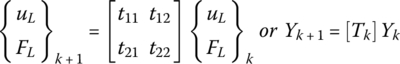
where Y and [Tk] denotes the state vector = {uL FL}T and the transfer matrix of the kth cell. Note that the transfer matrix relates the state vector at the left end of k + 1th cell to that at the left end of the kth cell. For exactly periodic structures, [Tk] is the same for all cells and Eq. (10.6) reduces to:
However, for aperiodic structures, [Tk] varies from cell to cell to appropriately account for the nature of aperiodicity.
10.2.2.2 Basic Properties of the Transfer Matrix
The transfer matrix [T] has very interesting characteristics and is called a “simplectic matrix.” Among these characteristics are:
- Determinant of [T] = 1:
Proof
From Eq. (10.5) and the symmetry of the dynamic stiffness matrix, we get:
(10.8)
- [T]−T = J [T] J−1

Proof
From Eq. (10.6);
(a)
But
(b)
From (a) and (b):
- Eigenvalues of [T] are λ and λ−1
Proof
The eigenvalue problem of [T] can be written as:
Equation (10.10) can be rewritten as:
where J =
 . Using Eq. (10.9) and let Xk = J Yk, then Eq. (10.11) reduces to:
or
Equation (10.12) indicates that λ−1 is an eigenvalue of the matrix [T]T that means that it is also an eigenvalue of the matrix [T]. The equation also indicates that Xk is the corresponding eigenvector. Accordingly, if λ and Yk are an eigenvalue and an eigenvector for [T] then λ−1 and Xk are companion eigenvalue and an eigenvector for [T].
- Mathematical Meaning of eigenvalue λ of [T]
Combining Eqs. (10.7) and (10.10) gives:
indicating that the eigenvalue λ of the matrix [T] is the ratio between the state vectors at two consecutive cells.
Hence, one can reach the following conclusions:
- If |λ| = 1 , then Yk + 1 = Yk and the state vector propagates along the structure as is. This condition defines a “pass band” condition.
and
- If |λ| < 1 , then Yk + 1 < Yk and the state vector is attenuated as it propagates along the structure. This condition defines a “stop band” condition.
A further explanation of the physical meaning of the eigenvalue λ can be extracted by rewriting it as:
where μ is defined as the “propagation constant,” which is a complex number whose real part (α) represents the logarithmic decay of the state vector and its imaginary part (β) defines the phase difference between the adjacent cells.
For example, rewriting Eq. (10.13) as:
and considering only the jth components
 of the deflection vector uL, at cells k and k + 1, which can be written as:
where
 denote the amplitude and phase shift of the jth component
  at the nth cell.
From Eqs. (10.15) and (10.16), we get:
Eq. (10.17) indicates that:

and

Therefore, the equivalent conditions for the pass and the stop bands can be written in terms of the propagation constant parameters (α and β) as follows:
- If α = 0 (i.e., μ is imaginary), then we have the “Pass Band” as there is no amplitude attenuation.
- If α ≠ 0 (i.e., μ is real or complex), then we have the “Stop Band” as there is amplitude attenuation defined by the value of α.
- Physical Meaning of the eigenvalues λ and λ−1 of [T]
A better insight into the physical meaning of the eigenvalues λ and λ−1 can be gained by considering the following transformation of the cell dynamics into the wave mode component domain:
where Φ is the eigenvector matrix of the transfer matrix [T]. Also, Wk is the wave mode component vector that has the right‐going wave component wr and left‐going wave component wL.

Substituting Eq. (10.18) into Eq. (10.7), it reduces to:

or

Note that the matrix Φ−1 [T] Φ reduces to the matrix of eigenvalues of the matrix [T], that is:
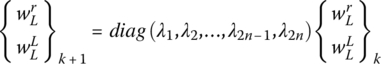
But, because of the particular nature of the eigenvalues of [T] as they appear in pairs (λ, λ−1), then this equation reduces to:

where
Equation (10.20) can be expanded to give:
For the jth component of w, we have:
that is, the eigenvalue λj is the ratio between the amplitude of the right‐going waves, whereas λj−1 defines the ratio between the amplitude of the left‐going waves as shown in Figure 10.6.

Figure 10.6 The propagation of right‐ and left‐going waves.
Therefore, if |λj| < 1, then the pair (λj,![]() ) define attenuation (or stop bands) along the wave propagation direction from cell k to cell k + 1. Also, if |λj| = 1, then the pair (λj,
) define attenuation (or stop bands) along the wave propagation direction from cell k to cell k + 1. Also, if |λj| = 1, then the pair (λj,![]() ) define propagation without attenuation (i.e., pass bands).
) define propagation without attenuation (i.e., pass bands).
One question remains here to be answered and that is: why the eigenvector matrix Φ transforms the state vector Yk = {uL FL}T to the wave mode component vector Wk = ![]() as governed by Eq. (10.18). An attempt to answer this question is illustrated in Example 10.1 for the case of rods undergoing longitudinal vibrations.
as governed by Eq. (10.18). An attempt to answer this question is illustrated in Example 10.1 for the case of rods undergoing longitudinal vibrations.
Solution
As the equation of motion of the rod is given by:
where u is the longitudinal deflection, ρ is the density and E is Young's modulus.
Then, assuming a solution: u = U(x) eiωt, reduces the equation of motion to:
or
where k = wave number = ![]() .
.
Equation (10.23) can be written in the following state‐space form:

that has a solution:

This solution can be put in a transfer matrix form by setting Ux = F/EA and extracting eAx using symbolic manipulation software (such as Mathematica) to give:

or,

Accordingly, the transfer matrix [T] is given by in a more compact form as:

where ![]() , which is called impedance of the rod.
, which is called impedance of the rod.
Using symbolic manipulation software (such as Mathematica) indicates that [T] has the following two eigenvalues:
Note that as λ1, 2 = e∓ikx = cos (kx) ∓ i sin(kx) then |λ1, 2| = 1, that is, defining pass band. This means that the uniform rod will transmit any incident waves without any attenuation.
Note also that λ2 is the reciprocal of λ1 to confirm property c of the transfer matrices as given in Section 10.2.2.2.
Symbolic manipulation software indicates also that [T] has the following two eigenvectors, which correspond to λ1,2, respectively:
v1 = {1 ‐EAki}T and v2 = {1 EAki}T with eigenvector matrix  .
.
Now, the eigenvector matrix Φ is used to define the following transformations:

The physical meaning of the vectors {w1 w2}xT and {w1 w2}0T will become apparent shortly.
The first part of Eq. (10.26) gives:
Combining Eqs. (10.24) with (10.26) gives, after some manipulation, the following expression:
Accordingly,
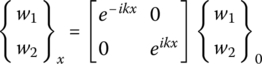
Hence, substituting for w1(x) and w2(x) from Eq. (10.29) into Eq. (10.27), it reduces to:
Equation (10.30) indicates that the longitudinal displacement u(x) consists of two wave components: one propagating to the right = w1(x) = e−ikx w1(0) and one propagating to the left = w2(x) = eikx w2(0). Therefore, the vector {w1 w2}xT physically denotes a vector = {wr wL}xT with wr(x) and wL(x) defining the right and left‐going waves at location x.
Note that the vector {wr wL}xT = {w1 w2}xT is generated from the vector {w1 w2}0T using the propagation Eq. (10.29) with {w1 w2}0T defining a vector = {wr wL}0T where wr(0) and wL(0) denote right‐ and left‐going waves at location 0.
A graphical representation of Eq. (10.29) is displayed in Figure 10.8.
In summary, the present example has proved that the eigenvector matrix Φ, of the transfer matrix [T], transforms the state vector Y = {u F}T to the wave mode component vector W = {wr wL}T as governed by Eq. (10.26) that is equivalent to Eq. (10.18).

Figure 10.7 Rod undergoing longitudinal vibrations.

Figure 10.8 Right and left‐going waves in rods.
Solution
The eigenvalues of {T] can be determined from
or
but as the det([T]) = 1, from Section 10.2.2.2.i, then this equation reduces to
Hence, from the theory of quadratic equations, the roots λ1 and λ2 of these equations must be such that:
But as λ1 = 1/λ2 = λ (Section 10.2.2.2.iii), and λ = eμ(as given by Eq. (10.14)), then
Solution
As
and
then,
or

10.3 Filtering Characteristics of Passive Periodic Structures
10.3.1 Overview
The methodologies for determining the pass and stop bands of passive periodic structures are introduced here. Illustrated examples are given to demonstrate the application of these methodologies to rods as examples of one‐dimensional periodic structures.
10.3.2 Periodic Rods in Longitudinal Vibrations
Consider the longitudinal vibrations of the periodic rods shown in Figure 10.9.

Figure 10.9 Passive periodic rods. (a) With geometrical discontinuity and (b) with material discontinuity.
These rods are made of assemblies of the periodic cells shown in Figure 10.10a,b. Each of these unit cells consists of two substructures a and b, which can be either of the same material with different cross sections (Figure 10.10a), or made of different materials with the same cross sections (Figure 10.10b).

Figure 10.10 Unit cells of passive periodic rods.
The dynamic characteristics of the individual substructure (a or b) can be described by its transfer matrix [Ts], as defined by Eq. (10.25), as follows:

Combining the transfer matrices of the substructures a and b, yields the transfer matrix [T] for the unit cell as follows:
The pass and stop bands characteristics of the periodic rod can be determined by investigating the eigenvalues of the transfer matrix [T] for different combinations of the longitudinal rigidities EsAs and dimensionless frequencies ksLs.
Solution
Figure 10.12a,b shows the magnitude of the eigenvalues of the transfer matrix [T] = [Tb] [Ta] as function of the frequency. The figures identify also the pass and stop bands for the two cases.
Note that the width and location of the stop and pass bands depends primarily on the physical and geometrical properties of the periodic rod.

Figure 10.11 Periodic rod with material and geometrical discontinuities.

Figure 10.12 Pass and stop bands of an elastic periodic rod. (a) Case 1 and (b) Case 2.
Solution
Figure 10.13 shows the magnitude of the eigenvalues of the transfer matrix [T] = [Tb] [Ta] as function of the frequency. The figure indicates that presence of damping in the periodic rod has resulted in eliminating the pass bands completely and extended the stop band over the considered frequency band.
In this example, the unit cell of the periodic structure is assumed to generically consist of an elastic substructure bonded to a viscoelastic substructure. Specifically, the latter substructure can be made of either a conventional viscoelastic material or a shunted piezoelectric network (Thorp et al. 2001).
Figure 10.13 Stop band of an elastic‐viscoelastic periodic rod.
10.4 Natural Frequencies, Mode Shapes, and Response of Periodic Structures
10.4.1 Natural Frequencies and Response
The modal parameters and the response of periodic structures can be determined using the transfer matrix approach presented in Section 10.3. The state vectors at the beginning and the end of the structure are related by the system transfer matrix [TN]:

where subscripts “o” and “N” denote, respectively, the beginning and the end of the periodic structure.
Equation (10.35) can be expanded as follows:
where {x0, xN} and {F0, FN} are the amplitudes of the displacements and forces at the beginning and the end of the structure.
Equation (10.36) can be used to extract the natural frequencies of the periodic structure after imposing the boundary conditions as listed in Table 10.1.
Table 10.1 Equations for computing the natural frequencies of periodic structures at different boundary conditions.
| No. | End 0 | End N | Conditions | Equations |
| 1 | Free | Free | F0 = 0 and FN = 0 | TN21 = 0 |
| 2 | Free | Fixed | F0 = 0 and xN = 0 | TN11 = 0 |
| 3 | Fixed | Free | x0 = 0 and FN = 0 | TN22 = 0 |
| 4 | Fixed | Fixed | x0 = 0 and xN = 0 | TN12 = 0 |
For example, for a structure fixed at end “N” and excited at its free end “0” by a harmonic force (f0), the displacement x0 at the free end and the force at the fixed end FN can be obtained from Eq. (10.36) as follows:
Equation (10.37) is used to determine the unknown displacement and force at the two ends of the structure, for the considered set of boundary conditions. The state vectors at any intermediate point can be now determined using the transfer matrices of the individual cells (Eq. (10.13)).
Solution
The transfer matrix of the substructures a and b are given, according to Eq. (10.33), by

and

where a = 4.818E‐6 and b = 1.732E‐4.
Accordingly, the transfer matrix [T] of the unit cell is given by

that is,
and
Then, using Eqs. (10.9) and (10.32), one can easily show that the transfer matrix [TN] of the entire rod is given by

with

The natural frequencies of the periodic rod can be determined, according to Table 10.1, from
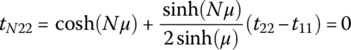
with t11 and t22 are as given by Eqs. (10.38) and (10.39).
Note that Eq. (10.40) is an equation in the frequency ω. Solution of Eq. (10.40) for the natural frequencies of the periodic rod requires a search for the frequencies that satisfy Eq. (10.40) with an additional constraint that these frequencies must lie within the pass bands of the periodic rod. Figure 10.14 shows a flow chart of the search procedure for the natural frequencies.

Figure 10.14 Search for the natural frequencies of the periodic rod.
Figure 10.15a shows the real part α of the propagation parameter μ as a function of the frequency and defines accordingly the pass band of the periodic rod. Within this band, the boundary condition given by Eq. (10.40) is displayed also as a function of the frequency in Figure 10.15b. The natural frequencies that satisfy Eq. (10.40) are marked on Figure 10.15b.

Figure 10.15 The logarithmic decay (a) and the natural frequencies (b) of the periodic rod.
Table 10.2 shows a comparison between the natural frequencies obtained using the theory of periodic structures and the theory of finite elements.
Table 10.2 The natural frequencies of the periodic rod (Hz).
| Mode | 1 | 2 | 3 | 4 | 5 | 6 | 7 | 8 |
| Theory of Periodic Structures | 55 | 164 | 269.5 | 370 | 462 | 542.5 | 609.6 | 657 |
| Finite Element Theory | 55.04 | 164.07 | 269.85 | 370.04 | 462.08 | 543.16 | 610.39 | 692.3 |
It can be seen that there is a close agreement between the predictions of the theory of periodic structures and the theory of finite elements.
For the sake of completion, Figure 10.16 shows the real part α of the propagation parameter μ and the boundary condition given by Eq. (10.40) for a uniform rod made of material a only. It is clear that the rod exhibits only a pass band as indicated in Example 10.1. The figure displays also the natural frequencies that satisfy Eq. (10.40). Within the considered frequency range, the first two modes are 2594.25 and 7783.2 Hz, as predicted by the theory of periodic structures, compared to 2595.04 and 7801.13 Hz, as predicted by the theory of finite elements.

Figure 10.16 The logarithmic decay (a) and the natural frequencies of a uniform rod (b).
10.4.2 Mode Shapes
Computation of the mode shapes corresponding to the natural frequencies obtained in Section 10.4.1 can be carried out using Eq. (10.36). For the case of a fixed‐free periodic rod, let x0 = 0 and F0 = 1 to give
withTN12(ωn) is the partitioned transfer matrix TN12 evaluated at the natural frequency ωn.
The state vectors at any intermediate point can now be determined using the transfer matrices of the individual cells (Eq. (10.32)) as follows

with k = N‐1, …, 1
The vector {x0, x1, .., xN}is the mode shape corresponding to the natural frequency ωn.
Solution
Figure 10.17 shows the mode shapes of the first four natural frequencies of the periodic rod as obtained by the theory of periodic structures and the theory of finite elements.
Figure 10.17 indicates excellent agreement between the predictions of the mode shapes by the theory of periodic structures and the theory of finite elements. Note that the piecewise linear behavior displayed in the figure is attributed to the fact that the deflections are computed only at the boundaries of the cells.

Figure 10.17 Mode shapes of the periodic rod.
10.5 Active Periodic Structures
In this section, the theory governing the operation of active periodic structures is introduced and numerical examples are presented to illustrate their tunable filtering and localization characteristics (Baz, 2001). The examples considered include periodic/aperiodic spring‐mass systems controlled by piezoelectric actuators.
The presented examples emphasize the unique potential of the active periodic structures in controlling the wave propagation both in the spectral and spatial domains in an attempt to stop/confine the propagation of undesirable disturbances.
10.5.1 Modeling of Active Periodic Structures
Figure 10.18a shows a periodic rod consisting of a stepped base structure which is augmented with active piezoelectric inserts placed periodically along the rod length. The idealized equivalent spring‐mass system, shown in Figure 10.18b, is made of identical cells each of which consists of an assembly of passive and active sub‐cells. Each sub‐cell consists of three masses connected and separated by a passive spring and an active piezoelectric spring as indicated in Figure 10.18c,d.


Figure 10.18 An active periodic spring‐mass system. (a) Original system, (b) equivalent system; (c) cell k; and (d) free‐body diagram of the unit cell.
The dynamics of such one‐dimensional periodic systems are determined using the classical transfer matrix method presented in Sections 10.2–10.4. The developed transfer matrices are utilized to determine the pass and stop bands, natural frequencies, mode shapes and frequency response of the system for different control gains and disorder levels generated by randomizing the control gains of the individual cells.
10.5.2 Dynamics of One Cell
Considering the free‐body diagram of one cell of the periodic spring‐mass system shown in Figure 10.18c; one can describe the dynamics of the passive and active sub‐cells as follows:
10.5.2.1 Dynamics of the Passive Sub‐Cell
The equation of motion of the passive sub‐cell is given by:

where m and ks are half the mass of the step and stiffness of the passive spring. These parameters are given by ![]() where t, b, and L denote the thickness, width, and length with subscripts m and s denote the mass and base structure, respectively. Also, x and F define the deflection and force with subscripts L and Is denoting the left and interface sides of the passive sub‐cell.
where t, b, and L denote the thickness, width, and length with subscripts m and s denote the mass and base structure, respectively. Also, x and F define the deflection and force with subscripts L and Is denoting the left and interface sides of the passive sub‐cell.
For a sinusoidal motion at a frequency ω, this equation of motion reduces to:

10.5.2.2 Dynamics of the Active Sub‐Cell
The constitutive equations of the active piezoelectric spring are given by (Agnes 1999):

where Ep, Dp, Tp, and Sp are the electrical field intensity, electrical displacement, stress, and strain of the piezo‐spring, respectively. Also, εs, hp, and CD define the electrical permittivity, piezo‐coupling constant, and elastic modulus.
Equation (10.42) can be rewritten in terms of applied voltage V, piezo‐force Fp, electrical charge Qp, and net deflection (xR − xI) as follows:

Eliminating the charge Qp from Eq. (10.43) gives:
Let the piezo‐voltage Vp be generated according to the following control law:
Then, Eq. (10.44) reduces to:

where ![]() with kpc and kps denoting the active piezo‐stiffness due to the control gain, Kg, and the structural piezo‐stiffness.
with kpc and kps denoting the active piezo‐stiffness due to the control gain, Kg, and the structural piezo‐stiffness.
Equation (10.46) can be used to generate the force vector {FIp FR}T acting on the piezo‐spring rewritten as:

with kp = (kpc + kps) is the total stiffness of the piezo‐spring.
Hence, the dynamic equations of sinusoidal motions of the active sub‐cell is given by:

10.5.2.3 Dynamics of the Entire Cell
The dynamics of the entire cell can be determined by the assembly of the dynamic equations of the passive and active sub‐cells that are given by Eqs. (10.41) and (10.48), respectively. This yields the following dynamic equations:
where FI = FIs + FIp denotes the total interface force.
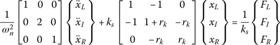
Using Guyan's reduction to eliminate the interface degree of freedom xI yields the following condensed dynamic equations:

where

with rk = kp/ks = stiffness ratio and ![]() = frequency ratio. Note that the stiffness ratio rk can be written as:
= frequency ratio. Note that the stiffness ratio rk can be written as:
where rks and rkc denote the structural stiffness ratio and the control stiffness ratio.
In Eq. (10.51), an additional subscript k is added to denote the dynamics of the kth cell.
10.5.2.4 Dynamics of the Entire Periodic Structure
The dynamics of the entire periodic structure can be determined by rearranging Eq. (11) to take the following form:

Consider now the compatibility and equilibrium conditions at the interface between the kth and the k + 1th cells, which yields the following expressions:
Substituting these conditions into Eq. (10.52), it reduces to:

In a more compact form, Eq. (10.54) can be rewritten as:

where Y and [Tk] denote the state vector = {xL FL}T and the transfer matrix of the kth cell. Note that the transfer matrix relates the state vector at the left end of k + 1th cell to that at the left end of the kth cell. For exactly periodic structures, [Tk] is the same for all cells and Eq. (10.55) reduces to:
However, for aperiodic structures, [Tk] varies from cell to cell to appropriately account for the nature of aperiodicity. In this section, the aperiodicity can be easily introduced by varying the control gain Kg. Such flexibility is made possible by providing the periodic structure with active control capabilities.
The wave propagation as well as the pass and stop band characteristics of the active periodic structure can be analyzed by studying the eigenvalues of the transfer matrix [T] using the approaches outlined in Sections 10.2–10.4.
Solution
The system Eqs. (10.50), (10.54–10.56) are used to compute the transfer matrix [T]. The eigenvalues λ of the matrix [T] are computed and plotted against the dimensionless frequency parameter, R.
Equation (10.14) is then used to compute the attenuation parameter α and the phase shift parameter β. These propagation parameters are plotted also against R.
The resulting characteristics are shown in Figure 10.19. Figure 10.19a displays the absolute of the eigenvalues (|λ|) of the transfer matrix [T] as a function of the dimensionless frequency R. The figure indicates that |λ| = 1 for R < 1.4 and |λ|≠ 1 for R > 1.4. Accordingly, the passive system has a pass band for R < 1.4 and a stop band for R > 1.4. In other words, the system acts as a “low pass” filter with a cut‐off frequency of 1.4.
For the sake of completion, Figure 10.19b and c are included to display the real and imaginary parts (α and β) of the propagation constant μ. It is very clear that for R < 1.4, the attenuation parameter α= 0, that is, the system has no apparent damping. This results in complete propagation of the waves or a “pass band.”
But for R > 1.4, the attenuation parameter α ≠ 0, that is, the system has an apparent damping that results in attenuating the propagation of waves in a manner equivalent to the presence of actual damping. This occurs over a broad frequency range that is called a “stop band.” Under these conditions, the system behaves as a “low pass filter.”

Figure 10.19 Filtering characteristics of the passive periodic spring‐mass system with rks = 1 and rkc = 0. (P = Pass band, S = Stop band).
Solution
Figure 10.20–d displays the corresponding filtering characteristics of the active periodic structure with the control gain Kg selected such that rkc = 2, 5, −0.75, and iR, respectively.
In Figure 10.20a,b, the filtering characteristics exhibit two pass bands and two stop bands. For example, when rkc = 5, the pass bands occur for 0 < R < 1 and 2.4 < R < 2.65, and the stop bands occur for 1 < R < 2.4 and 2.65 < R < ∞.
It is important to note that increasing Kg increases the width of the notch filtering and shifts the highest cut‐off frequency to a higher frequency R.
Figure 10.20c shows the corresponding characteristics when Kg is selected such that rkc = −0.75 indicating a positive proportional feedback control action. This action results in reducing the width of the notch filtering and shifts the highest cut‐off frequency to a lower frequency R.
With such simple adjustment of the control gain Kg, it would be possible to tune the filtering characteristics of the structure in response to external excitations in order to stop the propagation of these excitations along the structure.
It is worth noting here that the passive periodic structures have usually high cut‐off frequencies. Hence, the effectiveness of the passive periodic structures is limited only to the blocking of the propagation of high frequency excitations. But, once provided with active control capabilities, these cut‐off frequencies can be lowered considerably and the active structures become effective in stopping the propagation of low‐frequency excitations as well.
Figure 10.20d displays the filtering characteristics of the active periodic structure when rkc = iR indicating a negative derivative feedback. The figure indicates that structure exhibits stop band characteristics over the entire frequency range.

Figure 10.20 Filtering characteristics of the active periodic spring‐mass system with rks = 1 and for different values of rkc (P = Pass band, S = Stop band).
10.6 Localization Characteristics of Passive and Active Aperiodic Structures
10.6.1 Overview
In this section, the localization effects arising from the presence of unintentional irregularity (or disorder) in the geometrical parameters of the periodic structure are investigated. Particular emphasis is placed on studying the effect of the disorder levels and excitation frequencies on the response of the structure as well as on the extent of the achieved localization.
In this regard, the work of Mead and Lee (1984), Pierre (1988), Luongo (1992), Langley (1994), Mester and Benaroya (1995), and Mead (1996) present the necessary background and pioneering work in that area.
10.6.2 Localization Factor
The performance of the disordered periodic structure can be quantified using the “localization factor – γ.” The origin of the localization factor can best be understood by considering Figure 10.6 and rewriting Eq. (10.20) as follows

or,
Accordingly, the coefficients tL and tr have the physical meaning of the transmission coefficients associated with wave propagation from the left and right as well as the eigenvalue of the transfer matrix [T]. The matrix [S] is known as the “scattering matrix.”
For a periodic structure made of N cells, Eqs. (10.57) and (10.58) become

and
Equation (10.60) can be rewritten as
or
which reduces to
Equation (10.61) indicates that the “average logarithmic decay” in a periodic structure with N cells is the same as the logarithmic decay in the individual cell.
Note that the diagonal terms in the scattering matrix are zero for the case of a purely periodic structure. In the case of aperiodic structures, these terms become non‐zero, because the transfer matrices of the individual cells are no longer the same due to the irregularities. Hence, a matrix Φ that diagonalizes the nominal transfer matrix will not necessarily diagonalize the disordered transfer matrix and Eq. (10.59) takes the following form

with the coefficients ![]() and
and ![]() physically denoting the reflection coefficients associated with the left and right propagating waves.
physically denoting the reflection coefficients associated with the left and right propagating waves.
Due to the reflections at the interfaces of dissimilar cells, wave propagation in aperiodic chain is attenuated even if the excitation frequency is within the pass band and the system remains undamped. This is in contrast to periodic structures where the scattering matrix includes transmission matrices only.
The phenomenon of attenuation of wave propagation in aperiodic structures was reported first by Anderson (1958) in atomic lattices and then by Hodges (1982) in engineering dynamical systems.
The performance of the actively disordered periodic structure is quantified, for example, by using the localization factor – γ that is defined according to Cai and Lin (1991) as follows:

where λk is the eigenvalue of the kth cell. Also, according to Eq. (10.63), the localization factor γ defines the average exponential decay for an assembly of N cells. For a perfect periodic structure |λk| is constant for every cell. In a pass band, |λk| is equal to one and the localization factor is correspondingly equal to zero.
Equation (10.36) can be used to determine the unknown displacement and force at the two ends of the structure, for any considered set of boundary conditions. The state vectors at any intermediate point can be now determined using the transfer matrices of the individual cells (Eq. (10.33)).
The irregularity is introduced here by adding a disorder term to one or all of the geometrical parameters of the structure as, for example, the length of one of the sub‐cells such that:
where ![]() and
and ![]() denote the total and the nominal length of the kth sub‐cell. In Eq. (10.64), dk defines a random disorder that is normally distributed with zero mean and variance of σ.
denote the total and the nominal length of the kth sub‐cell. In Eq. (10.64), dk defines a random disorder that is normally distributed with zero mean and variance of σ.
Alternatively, the irregularity can be introduced by adding a disorder term to one or all of the control gain Kg of the individual sub‐cells such that:
where Kgk and ![]() denote the total and the nominal control gain of the kth sub‐cell. In Eq. (10.65), δKgk defines a random disorder which is normally distributed with zero mean and variance of σ.
denote the total and the nominal control gain of the kth sub‐cell. In Eq. (10.65), δKgk defines a random disorder which is normally distributed with zero mean and variance of σ.
Solution
The localization factor – γ is calculated for the aperiodic structure using Eq. (10.63) as follows:

where λk is the eigenvalue of the kth cell.
Figure 10.22 shows that the localization factor becomes different from zero within the confined boundaries of the stop bands.
Note that the localization factors concentrate at the boundaries of the stop bands, indicating that the disorder extends the range of frequency where longitudinal waves are attenuated. The width of the attenuating bands and the value of the localization factors increase with the level of disorder. In particular, Figure 10.22c shows that for high levels of irregularity, with σ= 3, the first and the second pass bands have been completely eliminated.

Figure 10.21 An active periodic rod.

Figure 10.22 Effect of disorder level (sigma = σ) on the localization factor (P = Pass band, S = Stop band). (a) σ = 0.25, (b) σ = 1 and (c) σ = 3.
Solution
From Eq. (10.36) with x0 = 0,
Eliminating F0 between these equations gives
This equation gives the displacement xN at the free end of the rod in terms of the magnitude of the input excitation force FN. The state vectors at any intermediate point can be now determined using the transfer matrices of the individual cells (Eq. (10.33)).
Figure 10.24 emphasizes that the vibration energy is spatially spread over the entire periodic structure and is confined to the zone near the excitation end for the aperiodic structure. This localization of the vibration energy is achieved easily by randomly distributing the control gain, rkc. Similar performance characteristics can, however, be obtained in passive periodic structures by randomly varying the geometric parameters of the different cells. But, this task is rather cumbersome to be practical.
The phenomenon of vibration localization is demonstrated also in Figure 10.25a,b for the excitation frequencies of R = 1.75 and 1.95. However, in these cases only small disorder levels (σ= 0.25) were necessary to stop the propagation of the waves along the structure. This again emphasizes the importance of providing structures with active control capabilities in order to tailor the disorder level to match the nature of the external excitation.

Figure 10.23 An active free‐fixed periodic rod with sinusoidal end loading.

Figure 10.24 Vibration localization at frequency R = 0.9 with disorder level σ=2.5 (periodic  , aperiodic
  ).
).

Figure 10.25 Vibration localization with disorder level σ = 0.25 (periodic  , aperiodic
  ). (a) R = 1.75 and (b) R = 1.95.
Solution
For general loading, Eq. (10.49) can be rewritten as:

Dividing by ks gives:
or

where

Now, the theory of finite elements can be utilized to assemble the overall mass and stiffness matrices [Mo] and [Ko] to formulate the overall equations of motion of the periodic rod. After imposing the boundary conditions, these equations can be written as follows:
where

Figure 10.26 An active free‐fixed periodic rod subject to an impulsive loading. (a) Periodic rod and (b) impulsive load at the free end.
Figures 10.27 and 10.28 show the characteristics of the passive and active periodic rods, respectively.


Figure 10.27 Characteristics of passive periodic rod (rkc = 0). (a) Deflection vs time, (b) PSD vs frequency, (c) wavelength vs frequency, and (d) frequency vs time.


Figure 10.28 Characteristics of active periodic rod (rkc = 5).(a) Deflection vs time, (b) PSD vs frequency, (c) wavelength vs frequency, and (d) frequency vs time.
In Figure 10.27a, the time response of the free end of the rod is shown while Figure 10.27b displays the corresponding Fast Fourier Transform (FFT) indicating a sharp drop in the response for frequencies R higher than 1.4. This indicates the presence of a stop band starting at R > 1.4. This result matches the predictions of the eigenvalues of the transfer matrix that are displayed in Figure 10.27c.
Figure 10.27d shows a spectrogram obtained by applying the continuous Morlet wavelet transform (WT), described in Appendix 10.A, in order to display the frequency content of the response of the free end of the rod as a function of time. It is evident that the spectrogram identifies clearly the modes of vibration of the rod and these modes coincide with those identified by the FFT as shown in Figure 10.27c.
Introducing the control action, with rkc = 5, has resulted in the characteristics shown in Figure 10.28. Figure 10.28a,b indicate a decrease in the amplitude of response of the rod both in the time and frequency domains. Such a decrease is evident for frequencies R < 1 due to the apparent damping resulting from operation within the stop band predicted by the eigenvalues of the transfer matrix in Figure 10.28c. Such apparent damping is quantified by the “attenuation parameter” α shown in Figure 10.20b. For values of 1 < R < 2, the “attenuation parameter” α reaches a peak plateau resulting in a significant attenuation of the wave propagation.
More importantly, Figure 10.28b shows also that high frequency modes appear around R = 2.4 where the active periodic rod has a pass band as can be identified clearly by the eigenvalues of the transfer matrix displayed in Figure 10.28c.
The spectrogram of Figure 10.28d identifies also the modes of vibration of the rod in a manner that conforms to those identified by the FFT as shown in Figure 10.28c.
10.7 Periodic Rod with Periodic Shunted Piezoelectric Patches
Shunted piezoelectric patches are periodically placed along rods, as shown in Figure 10.29, to control the longitudinal wave propagation in these rods. The resulting periodic structure is capable of filtering the propagation of waves over specified stop bands. The location and width of the stop bands can be tuned, using the shunting capabilities of the piezoelectric materials, in response to external excitations and to compensate for any structural uncertainty.

Figure 10.29 A rod with periodic shunted piezoelectric patches.
10.7.1 Transfer Matrix of a Plain Rod Element
The transfer matrix of the rod element of the ith cell is given by Eq. (10.25) as follows:

where ![]() = impedance of the rod element.
= impedance of the rod element.
It is evident from Eq. (10.66) that changing the material properties (Eri,ρri) or the geometry (Ari) along the rod length generates a discontinuity in the rod impedance. Controlling the impedance of periodic structures can modify the wave propagation characteristics along the rod.
10.7.2 Transfer Matrix of a Rod/Piezo‐Patch Element
The transfer matrix of the rod/piezo‐patch element of the ith cell can be obtained in a manner similar to the plain rod by using appropriate expressions for the wave number kci and impedance zci of the composite element such that Eq. (10.66) is modified to assume the following form:

where ![]() = impedance of the rod/piezo‐patch element.
= impedance of the rod/piezo‐patch element.
The wave number kci and impedance Zci of the composite element are determined using the “rule of mixtures” of composites such that:

and

where Ari and Api denote, respectively, the cross sections of the rod and of the piezo‐patch, ρri and ρpi are the densities of the rod and of the piezo, and Eri is the Young's modulus of the rod material. Also, ![]() denotes the complex modulus of the shunted piezo‐patch. It is determined by combining Eqs. (9.7) and (9.14) to yield:
denotes the complex modulus of the shunted piezo‐patch. It is determined by combining Eqs. (9.7) and (9.14) to yield:

where η = loss factor, ![]() = storage modulus,
= storage modulus, ![]() = Young's modulus of the unshunted piezo‐patch at open circuit,
= Young's modulus of the unshunted piezo‐patch at open circuit, ![]() = electromechanical coupling factor,
= electromechanical coupling factor, ![]() = capacitance at zero strain, s = Laplace complex number, and
= capacitance at zero strain, s = Laplace complex number, and ![]() = shunted impedance. For inductive‐resistive shunting
= shunted impedance. For inductive‐resistive shunting ![]() is given by:
is given by:
The values of shunting components L and R are determined to ensure optimal damping characteristics as outlined in Table 10.3 and as described in Sections 9.2.2.1 and 9.2.2.2.
Table 10.3 Optimal shunting parameters.
| Shunting Circuit | Resistive | Resistive/inductive |
| Tuning Frequency |
10.7.3 Transfer Matrix of a Unit Cell
The transfer matrix of a unit cell of a rod that is treated with periodically distributed piezo‐patches can be determined by combining Eqs. (10.66) and (10.67) to give:
Extracting the eigenvalues of the transfer matrix [Ti] will provide a means for identifying the wave propagation characteristics along the periodic rod with piezo‐patches.
Solution
Equations (10.66–10.72) are used to compute the transfer matrix of the unit cell of the periodic rod with piezo‐patches for different shunting strategies. The corresponding eigenvalues of the transfer matrix are determined and the attenuation and phase shift parameters (α and β) are extracted using Eq. (10.14).
Figure 10.30 displays the effect of the shunting strategies on the attenuation parameterα. In Figure 10.30a, the effect of the shunting resistance R on α is shown when the shunting inductance L = 0. It can be seen that increasing R beyond 25 Ω results in insignificant improvement in the attenuation parameter α. The effect of the shunting inductance L on the attenuation parameter α is displayed in Figure 10.30b when the shunting resistance R is maintained at 25Ω. A peak attenuation parameter value is obtained when L = 0.4 mH.
Figure 10.31 displays the attenuation and phase shift parameters (α and β) when the piezo‐patches are shunted using R = 25 Ω and L = 0 H along with the corresponding parameters of the unshunted piezo‐patches for comparison.
It can be seen that the periodic rod with unshunted piezo‐patches has three stop bands as marked in Figure 10.31. However, providing the piezo‐patches with resistive shunting has resulted in stopping wave propagation over the considered frequency band as the attenuation parameter α > 0 over the entire range.
Using an inductive and resistive shunting circuit with R = 25 Ω and L = 0.4 mH has improved the attenuation parameter over the considered frequency band as shown in Figure 10.31.

Figure 10.30 A rod with periodic shunted piezoelectric patches. (a) Effect of R only and (b) effect of L with R = 25Ω.

Figure 10.31 Propagation constants for resistive shunting ( R = 0Ω,
  R = 25Ω).

Figure 10.32 Propagation constants for resistive/inductive shunting (R = 0Ω and L = 0 mH,
  R = 25Ω L = 0.4 mH).
Table 10.4 Geometrical and physical properties of a rod.
| Young's modulus (N/m2) | Density (kg/m3) | Length (cm) | Width (cm) | Thickness (cm) |
| 3.6E9 | 1726 | 57.9 | 7.24 | 1.2 |
Table 10.5 Geometrical and physical properties of piezoelectric patches.
| Young's modulus (N/m2) | Density (kg/m3) | Length (cm) | Width (cm) | Thickness (cm) | Coupling factor k31 | Capacitance CSpi (nF) |
| 6.2E10 | 7800 | 7.24 | 7.24 | 0.0267 | 0.44 | 390 |
10.8 Two‐Dimensional Active Periodic Structure
10.8.1 Dynamics of Unit Cell
Figures 10.33 and 10.34 show an idealized 2D active periodic structure. The idealized structure is a spring‐mass system consisting of a two‐dimensional array of masses that are coupled by a set of active and passive springs. The active springs are placed in a periodic manner along the x‐axis. Such a placement strategy is considered to illustrate the characteristics of the 2D periodic structure. Similar characteristics can be obtained with other periodic placements of the active springs.

Figure 10.33 A 2D periodic spring‐mass system.

Figure 10.34 Deflections and forces acting on a unit cell.
In the considered spring‐mass system, a mass located at the ith row and jth column, has a single degree of freedom wij in the out‐of‐the x–y plane direction. The spectral equation of motion of that mass can be written, at a frequency ω, as
Similar equations of motion can be written for the other four nodes in unit cell can be obtained.
In Eq. (10.73), ks and kp denote the stiffness of the passive and active springs, respectively. Note that kp is defined as the sum of the stiffness components of the active spring due to its structural rigidity kps and control gain kpc, respectively, that is,
This definition implies that the active spring generates a force ![]() by feeding back the spring deflection as follows:
by feeding back the spring deflection as follows:
Hence, kpc defines in effect the gain of the controller.
Let rk be the ratio of the active to the passive stiffness, then
where rks and rkc denote the structural stiffness ratio and the control stiffness ratio respectively.
Equations (10.73–10.76) can be used to assemble the equation of motion of the entire cell to yield the following matrix equation
where

and

with the vectors {q} and {F} denote the deflection and force vectors as defined in Figure 10.34 and are given by

and

10.8.2 Formulation of Phase Constant Surfaces
The propagation of plane wave motion through two‐dimensional periodic structures is described according to Bloch's Theorem (Hussein 2009; Hussein et al. 2014) as follows
where μx and μy are propagation constants. Also, nx and ny denote integers that represent the position of the unit cell within the structure as shown in Figure 10.35.

Figure 10.35 Schematic drawing of a two‐dimensional periodic.
The propagation constant, μ, can be written in the form μj =αj + jβj, where αj and βj are attenuation and phase constants, respectively. Unlike in the case of one‐dimensional periodic structure, it is difficult to present graphically the complete range of possible values of μx and μy as functions of frequency. For this reason, results are normally presented only for the pass bands of the structure, which are described in terms of “phase constant surfaces” on which μx and μy are purely imaginary (i.e., αx =αy = 0). The usual analysis approach is to specify the phase constants βx and βy and then solve for the wave propagation frequency, ω. There are multiple solutions for ω at each combination ofβx and βy, and therefore solutions produce a series of “phase constant surfaces.”
In two‐dimensional periodic structures, stop bands are identified by the existence of frequency gaps between two consecutive phase constant surfaces. The evaluation and analysis of the phase constant surfaces therefore provides the tools required to fully analyze wave propagation in two‐dimensional periodic structures, and to explore their application as mechanical filters capable of impeding or confining the propagation of waves in limited regions of the structures.
To generate the multiple phase constant surfaces, the wave motion is characterized by the Bloch's relationships that relate the deflections and forces at the edges of a unit cell to the corresponding deflections and forces at the edges of the adjacent cells as follows:
and
Equation (10.81) is used to condense the original deflection and force vectors, {q} and {F}, to the reduced‐order {qr} and {Fr}, as follows:
where {qr} = {q1 q2 q3 q4 q5 q7 q8 q9}T and {Fr} = {F1 F2 F3 F4 F5 F7 F8 F9}T with the matrix [A] defined as follows

Then, the equation of motion (10.77) reduces to
where the reduced mass and stiffness matrices of the cell are defined in terms of the propagation constant pair μx and μy as [M]r = [A]*T [M][A] and [Kr] = [A]*T[K][A]. The values of the frequency corresponding to an assigned pair of propagation constants can be obtained by solving the following eigenvalue problem
Multiple solutions of the eigenvalue problem are presented in terms of “phase constant surfaces.”
10.8.3 Filtering Characteristics
The filtering characteristics of the two‐dimensional periodic structure are obtained by solving the eigenvalue problem, given by Eq. (10.85), for different values of the purely imaginary propagation constants ranging between 0 and π. The obtained solutions are used to generate the “phase constant surfaces” that define the frequencies corresponding to free wave propagation as well as the pass and stop bands of the two‐dimensional periodic structure.
Solution
The resulting characteristics are presented in Figure 10.36 as quantified by the phase constant and directivity plots. Figure 10.36a shows the propagation surfaces with the gaps between them indicating the stop bands. In Figure 10.36b, the dotted areas indicate pass bands while the white gaps between two consecutive pass bands indicate stop bands.
It can be seen that the locations of stop and pass bands are dependent on the direction of wave propagation, θ = tan−1 (βx/βy), which demonstrates that the two‐dimensional periodic structures can be utilized as directional mechanical filters.

Figure 10.36 Filtering characteristics of the passive periodic structure with rks = 1 and rkc = 0. (a) Phase constant surfaces and (b) directivity plot.
Solution
Figures 10.37 and 10.38 display the corresponding filtering characteristics of the resulting active periodic structure with rkc = 2 and 5 respectively indicating negative proportional feedback control action.
In these cases, the filtering characteristics that are quantified by the spectral width and directivity of the stop bands can be controlled by proper selection of the control gain rkc.
It is evident that increasing rkc increases the width of the stop bands significantly in all the wave propagation directions.

Figure 10.37 Filtering characteristics of the active periodic structure with rks = 1 and rkc = 2. (a) Phase constant surfaces and (b) directivity plot.

Figure 10.38 Filtering characteristics of the active periodic structure with rks = 1 and rkc = 5. (a) Phase constant surfaces and (b) directivity plot.
10.9 Periodic Structures with Internal Resonances
In this section, a special class of periodic structures is introduced because of their unusual response to elastic wave propagation as has been recently reported, for example, by Liu et al. (2005); Milton and Willis (2007); Huang and Sun (2011); Zhou and Hu (2013); and Hussein and Frazier (2013). This class of structures consists of rigid base structures containing cavities which house resonating masses connected to the cavity wall by springs. The macroscopic dynamical properties of the resulting periodic structures depend on the resonant properties of substructures that contribute to the rise of interesting effects such as broad stop band characteristics.
Figure 10.39 shows typical schematic drawings of a 1D conventional periodic structure and a 1D periodic structure with local resonances.

Figure 10.39 Periodic structures with and without local resonances: (a) conventional periodic structure and (b) periodic structure with local resonances.
The effect of introduction of the local resonances on the dynamic characteristics of these periodic structures can be understood by considering the unit cells shown in Figure 10.40 and extracting the eigenvalues of the corresponding transfer matrices using the approaches outlined in Sections 10.2–10.4.

Figure 10.40 Unit cells of periodic structures with and without local resonance. (a) Unit cell of a conventional periodic structure, (b) equivalent mass of mass‐in‐mass system, and (c) unit cell of a periodic structure with local resonator.
10.9.1 Dynamics of Conventional Periodic Structure
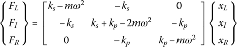
The equations of motion of the conventional periodic structure are given by:

or
where m1 and m2 denote the periodic masses as shown in Figure 10.40a. Also, k1 and k2 denote the stiffness of the periodic springs connecting these masses. The independent degrees of freedom of the system are X = {xL, xi, xR}T as displayed in Figure 10.40b. Note that [M], [K], and {F} define the overall mass matrix, stiffness matrix, and load vector of the unit cell.
Using the static condensation method to condense the internal degree of freedom xi gives:

Hence, the entire vector of independent degrees of freedom of the system can be constructed from the boundary degrees of freedom {xL xR}T as follows:

Using the transformation matrix TR, as defined in Eq. (10.88), the dynamics of the conventional periodic structure are condensed, for sinusoidal excitation at a frequency ω, to the following form:

or

Then, the transfer matrix Tc of the conventional periodic structure is given by:

10.9.2 Dynamics of Periodic Structure with Internal Resonances
10.9.2.1 Equivalent Mass. Of the Mass‐In‐Mass Arrangement
In order to derive the equations of motion of the periodic structure with internal resonances, it is essential to extract the equivalent mass of the mass‐in‐mass arrangement as shown in Figure 10.40b.
The equations of motion of the mass‐in‐mass arrangement are:
and
Assuming sinusoidal motion with F = F0 sin ωt, x1 = X1 sin ωt, and x2 = X2 sin ωt. Then, eliminating the internal degree of freedom x2, this results in:

This means that the two‐degree‐of‐freedom mass‐in‐mass arrangement behaves as a single‐degree‐of‐freedom system with an equivalent mass meq given by:

10.9.2.2 Transfer Matrix of the Mass‐In‐Mass Arrangement
The equations of motion of the unit cell shown in Figure 10.40c, using the equivalent mass, are given by:

For sinusoidal excitation at a frequencyω, Eq. (10.93) reduces to:

In a more compact form, Eq. (10.94) can be written as:

Then, the transfer matrix Ti of the periodic structure with internal resonances is given by:

Solution
Using the transfer matrices Tc and Ti given by Eqs. (10.90) and (10.96), the eigenvalues are computed for different excitation frequencies. Figures 10.41a and (10.41b) display these eigenvalues and identify the pass and stop bands of both the conventional periodic structure and the periodic structure with internal resonances.
The displayed results indicate that using periodic structure with internal resonances results in enhancing the stop band characteristics compared to those obtained with conventional periodic structures.

Figure 10.41 Filtering characteristics of periodic structures with and without local resonance. (a) m2 = 0.1 and (b) m2 = 0.025.
Solution
Figure 10.43 shows a finite element model of a unit cell of the metameterial plate with periodic local resonances. The model consists primarily of quadrilateral square plate elements of dimensions Le ×Le ×t. The theory of modeling this class of plates has been presented in Section 4.7 for the general case when it is treated with constrained VEM. In this section, the plate is considered to a plain plate which is totally untreated.
Figure 10.44 displays unit cell along with its eight neighboring cells in order to enable the computation of the propagation surfaces and directivity plots of plain aluminum plate and for the periodic plate with internal resonance sources as outlined in Section 10.8.2.
Figure 10.45a shows the propagation surfaces computed for the unit cell displayed in Figure 10.43, consisting of an aluminum base with a viscoelastic membrane that houses a local mass, for a frequency range from 0 to 8 kHz. A planar view of these surfaces is shown in Figure 10.45b. A large stop band is observed between 1.5 and 5.9 kHz.
Figure 10.46 shows a close‐up of the low‐frequency range of the propagation surfaces. The gaps between these surfaces in the 0–1 kHz range can be noticed between 200 and 215, 390 and 450, between 610 and 720 Hz, and once again between 790 and 900 Hz.
Figure 10.47 shows the propagation surfaces mathematically computed for a structure built from a plain cell, which acts as a datum for comparison purposes. For a conventional metal plate, waves should be able to propagate freely in both directions across the plate at any excitation frequency. This is shown clearly by the overlapping propagation surfaces throughout the entire considered frequency range allowing for no gaps between the surfaces to extend along the 0–2π range of βx or βy.
Figure 10.48 shows the vibration pattern of the metamaterial plate with the periodic local resonances when subject to an external excitation over the frequency range between 395 Hz until 460 Hz in the transverse z‐direction. This range corresponds to the first low‐frequency stop band range highlighted in Figure 10.45. It can be seen that this corresponds to the first natural mode of many of the local resonators. Hence, a large fraction of the vibration energy propagates directly into the locally resonant masses, which act as local absorbers of vibration, and thereby relieving the base structure completely from the vibration.
The frequency‐dependent directional behavior of the wave propagation in this class of structures can be visualized by using the polar plots such as those displayed in Figures 10.49a and 10.49b. In these diagrams, referred to as the directivity plots, the vibration frequency is plotted as a function of θ that is a measure of the direction of wave propagation given bytan−1(βx/βy). Frequencies are quantified by directivity plots as constant radii circles, and hence a stop band frequency is indicated by a circle that does not contain a solution for θ along its entire circumference, as can be seen in Figure 10.49a. Finally, Figure 10.49b shows the directivity of wave propagation in a plain aluminum cell for comparison. As expected, it can be seen that for any chosen frequency, that is, any constant radius circle, there has to exist at least one solution for θ along the circle's perimeter.
Note that if the physical properties of the individual unit cells can be tuned, this class of metamaterial structures can be used to confine/block wave propagation at the developed stop bands, as shown here, as well as steer the propagating waves within the pass bands through this directional filtering mechanism.

Figure 10.42 Metamaterial plate with periodic local resonances.

Figure 10.43 Finite element model of a unit cell of the metamaterial plate with periodic local resonances.

Figure 10.44 Periodic cells and mapping relations of the metamaterial plate (L = left, R = right, T = top, B = bottom).

Figure 10.45 (a) 3D and (b) 2D plots of the propagation surfaces for a metamaterial plate with periodic local resonances for frequencies up to 8 kHz.

Figure 10.46 (a) 3D and (b) 2D plots of the propagation surfaces for a metamaterial plate with periodic local resonances for frequencies up to 1 kHz.

Figure 10.47 Propagation surfaces for a plain aluminum plate for vibration frequencies up to 8 kHz showing complete absence of stop bands.

Figure 10.48 Vibration of the metamaterial plate with periodic local resonances during the first low‐frequency stop band.

Figure 10.49 Directivity plots for the plate with (a) periodic local sources of resonance and (b) the plain aluminum plate for frequencies up to 8 kHz.
Table 10.6 Main geometrical parameters of the periodic metamaterial plate.
| Length | b | Lc | Lr | Lg | L | Thickness (t) of plate and masses |
| Value (cm) | 15.2 | 5.1 | 1.3 | 1.3 | 20.3 | 0.1524 |
10.10 Summary
The dynamic characteristics of passive and active periodic structures are presented using the transfer matrix method. The theory governing the dynamics of these structures is introduced in order to demonstrate their unique mechanical filtering capabilities for wave propagation. As a result of these characteristics, waves are shown to propagate along the periodic structures only within specific frequency bands called the pass bands and wave propagation is completely blocked within other frequency bands called the stop bands. The spectral width and location of these bands are shown to be fixed for passive periodic structures, and tunable in response to the structural vibration for active periodic structures.
References
- Agnes G., “Piezoelectric coupling of bladed‐disk assemblies”, Proceedings of the Smart Structures and Materials Conference on Passive Damping (ed. T. Tupper Hyde), Newport Beach, CA, SPIE‐Vol. 3672, pp. 94–103, 1999.
- Anderson, P.W. (1958). Absence of diffusion in certain random lattices. Physical Review 109: 1492–1505.
- Baz, A. (2001). Active control of periodic structures. ASME Journal of Vibration and Acoustics 123: 472–479.
- Brillouin, L. (1946). Wave Propagation in Periodic Structures, 2e. Dover.
- Cai, G. and Lin, Y. (1991). Localization of wave propagation in disordered periodic structures. AIAA Journal 29 (3): 450–456.
- Chen, T., Ruzzene, M., and Baz, A. (2000). Control of wave propagation in composite rods using shape memory inserts: theory and experiments. Journal of Vibration and Control 6 (7): 1065–1081.
- Chui, C.K. (1992). An Introduction to Wavelets. In: Wavelets Analysis and Applications, vol. 1. Academic Press Inc.
- Cremer, L., Heckel, M., and Ungar, E. (1973). Structure‐Borne Sound. New York: Springer‐Verlag.
- Faulkner, M. and Hong, D. (1985). Free vibrations of a mono‐coupled periodic system. Journal of Sound and Vibration 99 (1): 29–42.
- Gopalakrishnan, S. and Mitra, M. (2010). Wavelet Methods for Dynamical Problems: With Application to Metallic, Composite, and Nano‐Composite Structures. CRC Press.
- Hodges, C.H. (1982). Confinement of vibration by structural irregularity. Journal of Sound and Vibration 82 (3): 441–444.
- Hodges, C.H. and Woodhouse, J. (1983). Vibration isolation from irregularity in a nearly periodic structure: theory and measurements. Journal of Acoustical Society of America 74 (3): 894–905.
- Huang, H.H. and Sun, C.T. (2011). A study of band‐gap phenomena of two locally resonant acoustic metamaterials”, Proceedings of IMechE Part N. Journal Nanoengineering and Nanosystems 224: doi: 10.1177/1740349911409981.
- Hussein, M.I. (2009). Theory of damped Bloch waves in elastic media. Physical Review B 80: 212301.
- Hussein, M.I. and Frazier, M.J. (2013). Metadamping: an emergent phenomenon in dissipative Metamaterials. Journal of Sound and Vibration 332: 4767–4774.
- Hussein, M.I., Leamy, M.J., and Ruzzene, M. (2014). Dynamics of Phononic materials and structures: historical origins, recent progress, and future outlook. Applied Mechanics Reviews 66 (4): 040802–(1–38).
- Langley, R.S. (1994). On the forced response of one‐dimensional periodic structures: vibration localization by damping. Journal of Sound and Vibration 178 (3): 411–428.
- Liu, Z., Chan, C.T., and Sheng, P. (2005). Analytic model of phononic crystals with local resonances. Physical Review B 71: 014103.
- Luongo, A. (1992). Mode localization by structural imperfections in one‐dimensional continuous systems. Journal of Sound and Vibration 155 (2): 249–271.
- Mead, D.J. (1970). Free wave propagation in periodically supported, infinite beams. Journal of Sound and Vibration 11 (2): 181–197.
- Mead, D.J. (1971). Vibration response and wave propagation in periodic structures. ASME Journal of Engineering for Industry 93: 783–792.
- Mead, D.J. (1986). A new method of analyzing wave propagation in periodic structures; applications to periodic Timoshenko beams and stiffened plates. Journal of Sound and Vibration 114 (1): 9–27.
- Mead, D.J. (1996). Wave propagation in continuous periodic structures: research contributions from Southampton. Journal of Sound and Vibration 190 (3): 495–524.
- Mead, D.J. and Bardell, N.S. (1987). Free vibration of a thin cylindrical shell with periodic circumferential stiffeners. Journal of Sound and Vibration 115 (3): 499–521.
- Mead, D.J. and Lee, S.M. (1984). Receptance methods and the dynamics of disordered one‐dimensional lattices. Journal of Sound and Vibration 92 (3): 427–445.
- Mead, D.J. and Markus, S. (1983). Coupled flexural‐longitudinal wave motion in a periodic beam. Journal of Sound and Vibration 90 (1): 1–24.
- Mead, D.J. and Yaman, Y. (1991). The harmonic response of rectangular sandwich plates with multiple stiffening: a flexural wave analysis. Journal of Sound and Vibration 145 (3): 409–428.
- Mester, S. and Benaroya, H. (1995). Periodic and near periodic structures: review. Shock and Vibration 2 (1): 69–95.
- Milton, G.W. and Willis, J.R. (2007). On modifications of Newton's second law and linear continuum elastodynamics. Proceedings of the Royal Society of London Series A 463: 855–880.
- Nouh, M., Aldraihem, O., and Baz, A. (2015). Wave propagation in metamaterial plates with periodic local resonances. Journal of Sound and Vibration 341: 53–73.
- Pierre, C. (1988). Mode localization and eigenvalue loci veering phenomena in disordered structures. Journal of Sound and Vibration 126 (3): 485–502.
- Roy, A. and Plunkett, R. (1986). Wave attenuation in periodic structures. Journal of Sound and Vibration 114 (3): 395–411.
- Ruzzene, M. and Baz, A. (2000). Control of wave propagation in periodic composite rods using shape memory inserts. ASME Journal of Vibration and Acoustics 122: 151–159.
- Ruzzene, M. and Baz, A. (2001). Active control of wave propagation in periodic fluid-loaded shells. Smart Materials and Structures 10 (5): 893–906.
- Sen Gupta, G. (1970). Natural flexural waves and the normal modes of periodically‐supported beams and plates. Journal of Sound and Vibration 13: 89–111.
- Thorp, O., Ruzzene, M., and Baz, A. (2001). Attenuation and localization of wave propagation in rods with periodic shunted piezoelectric patches. Journal of Smart Materials & Structures 10: 979–989.
- Zhou, X. and Hu, G. (2013). Dynamic effective models of two‐dimensional acoustic metamaterials with cylindrical inclusions. Acta Mechanica 224: 1233–1241.
10.A The Wavelet Transform
The WT of a signal x(t) is an example of a time‐scale decomposition obtained by dilating and translating along the time axis a chosen analyzing function (wavelet) (Chui 1992; Gopalakrishnan and Mitra 2010). The integral or continuous WT relative to some basic wavelet ψ(t) is defined as:

where b is a translation parameter used for positioning the function ψ(t) over the time domain, and a > 0 is a scaling parameter dilating or contracting the function ψ(t). The WT provides a flexible time‐frequency window, which automatically narrows when observing high frequency phenomena and widens when studying low‐frequency components (Chui 1992). The wavelet function used in this work is the Morlet wavelet, defined in the time domain as:
The Morlet wavelet is a sinusoidal function, oscillating at the frequencyωw, modulated by a Gaussian envelope of unit variance. Being composed of a modulated sinusoidal function, the Morlet wavelet is well suited for reproducing and analyzing signals in many applications.
As signal decomposition, the WT cannot be directly compared to a time‐frequency representation. However, it can be shown that b represents a time parameter and that the dilation parameter a is strictly related to frequency. In the frequency domain, the Morlet wavelet becomes:
Equation (10.A.3) shows that the frequency domain formulation of the Morlet wavelet is a Gaussian function centered at ω = ωw . Its dilated version is expressed as:
whose maximum is located at a ω = ωw. Since ωw = 1.875 π is a fixed parameter defining the wavelet function, the center of the Gaussian curve and therefore the frequency of the analysis can be located by changing the dilation parameter as follows:
The scale parameter can be hence considered as the inverse of a frequency parameter and thus the WT can be classified as a time‐frequency transform.
An alternative formulation of the continuous WT can be obtained transforming both the signal x(t) and the wavelet function ψ(t)in the frequency domain:

with X(ω) and ![]() being the Fourier transforms of x(t) and
being the Fourier transforms of x(t) and ![]() , respectively.
, respectively.
This formulation of the WT can be expressed in a discrete form as:

where fn is the discrete frequency and Δ a and Δ b are discrete increments of dilation and translation parameters. Equation (10.A.7) allows an easy implementation of the WT. The frequency domain formulation of the WT is particularly convenient when the signal to be analyzed is expressed in the frequency domain.
Problems
- 10.1 Consider the periodic spring‐mass system shown in Figure P10.1a, determine the first three natural frequencies of the system using the symmetric and asymmetric configurations shown in Figures P10.1b,c. Consider the system to be a. fixed‐free and b. free‐free. Compare the results of the considered configurations.
Determine also the mode shapes corresponding to the different natural frequencies assuming the system to consist of 50 cells (N = 50). Comment on the shape of the system transfer matrix for both the symmetric and asymmetric configurations.
Figure P10.1 (a–c) A periodic spring‐mass system.
- 10.2 For the spring‐mass system of Problem P10.1, determine and plot the distribution of the longitudinal displacement along the system. Assume that the system is fixed‐free and that it is excited by a unit sinusoidal force applied at its free end. Consider three excitation frequencies coinciding with the first three natural frequencies of the system.
- 10.3 Consider the periodic spring‐mass system shown in Figure P10.2, show that if the equation of motion of the nth mass is given by:

and the deflection un is given by: un = u0 ei(nka − ωt), where k = wave number, a = spacing between masses, ω = frequency, and t = time, then:

describes the dispersion relationship of the periodic spring‐mass system as shown in Figure P10.3.
Show also that for short wave number k, then the wave propagation is non‐dispersive with the following linear relationship between ω–k as shown in Figure P10.3:


Figure P10.2 Mono‐atomic periodic spring‐mass system.

Figure P10.3 The dispersion relationship of the mono‐atomic periodic spring‐mass system.
- 10.4 Consider the diatomic periodic spring‐mass system shown in Figure P10.4, show that if the equations of motion of the masses mA and mB are given by:

and

and the deflections u2n and u2n + 1 are given by:

where k = wave number, a = spacing between masses, ω = frequency, and t = time, then:

describes the dispersion relationship of the periodic spring‐mass system as shown in Figure P10.5 with roots ω1,2. Note that:
 is denoted by the effective mass. Also, the high frequency root ω1 is denoted by the “optical mode” and the low‐frequency root ω2 is called the “acoustical mode.”
Figure P10.4 A diatomic periodic spring‐mass system.

Figure P10.5 The dispersion relationship of the bi‐atomic periodic spring‐mass system.
- 10.5 Consider the periodic rod shown in Figure P10.6a, determine the natural frequencies of the entire system assuming the rod to be fixed‐free and consists of 50 cells (N = 50). Use the asymmetric configurations shown in Figure P10.6b.
Determine and plot the distribution of the longitudinal displacement along the system. Assume the system to be excited by a unit sinusoidal force applied at its free end. Consider three excitation frequencies coinciding with the first three natural frequencies of the system.

Figure P10.6 A periodic rod with material discontinuities.
- 10.6 For the periodic rod of Figure P10.6, assume that the impedance ratio za/zb varies along the rod in a normal random manner with zero mean and standard deviation σ. Determine and plot the distribution of the longitudinal displacement along the system. Assume the system to be excited by a unit sinusoidal force applied at its free end. Consider three excitation frequencies coinciding with the first three natural frequencies of the system. Assume different values of σ and determine the decay parameter γ as a function of σ.
- 10.7 Figure P10.7a shows a schematic drawing of the shear mode periodic mount that is made of identical cells in the longitudinal direction. Each cell can be divided into four elements (parts). These elements are numbered 1,2,3,4 from the right to the left as shown in Figure P10.7b. When the mount is subjected to longitudinal loading F, it deflected and assumes the configuration shown in Figure (P10.7c). The shear strain γ in the viscoelastic material is given by: where u1 and u3 are the longitudinal deflections of the aluminum core and outer aluminum layer, respectively. Also, h2 defines the thickness of viscoelastic layer between the aluminum core and the outer layer.
Using the theory of finite elements, derive the equations of motion for the elements and determine the transfer matrix of the unit cell.

Figure P10.7 A schematic drawing of the shear mode periodic mount.

Figure P10.8 A periodic shear mount as vibration isolator.
- 10.8 Consider the periodic shear mount shown in Figure (P10.8) is used to isolate the vibration of a payload mounted on the top platform from being transmitted to the foundation.
The periodic mount is manufactured from an aluminum base material and a viscoelastic core (VEM) that have the geometrical and physical properties listed in Tables P10.1 and P10.2.
Using the transfer matrix developed in problem P10.7, determine the attenuation parameter α as function of the excitation frequency and extract the pass and stop band characteristics of the mount.
Table P10.1 Geometric properties.
Length (mm) Thickness (mm) L1 4.76 h1 3.17 L2 17.46 h2 3.18 L3 4.76 h3 3.18 L4 3.18 b 25.4 Table P10.2 Physical properties.
Material Density (kg/m3) Modulus (MPa) Aluminum 2700 70,000a Viscoelastic layer 1201.4 9.193 + 4.596ib a Young's modulus.
b Complex shear modulus (G(1 + ηi), η = 0.5).
- 10.9 The periodic beam cell shown in Figure P10.9 consists of two sections such that each section is modeled by a single finite element. The physical and geometrical parameters of the two sections are: ma = 1 kg/m, EIa = 1 Nm2, La = 0.025 m, mb = 1 kg/m, EIb = 2 Nm2, and Lb = 0.025 m.
If the dynamic stiffness matrices KDa and KDb of the two sections are given by:

where

with i = a, b
Determine the transfer matrices of each section ([Ta], [Tb]) and of the unit cell ([T] = [Tb] [Ta]). Show that the plot of the absolute value of the eigenvalues of [T] as function of the frequency ω is as shown in Figure P10.10.

Figure P10.9 A periodic beam cell.

Figure P10.10 A plot of the absolute value of the eigenvalues of transfer matrix of a beam unit cell.
- 10.10 The periodic beam cell shown in Figure P10.9 consists of two sections (a, b) such that each section is modeled by the following distributed‐parameter model:

where
 . Put this distributed‐parameter model into the following state‐space model:
Show that the state‐space model can be reduced to the following transfer matrix formulation:

where
 with the matrix Ai given by:
Also, Yx and Y0 are the state vectors given by:

with M and V denoting the bending moment and shear force given by:

Determine the transfer matrices of each section ([Ta], [Tb]) and of the unit cell ([T] = [Tb] [Ta]). Show that the plot of the absolute value of the eigenvalues of [T] as function of the frequency ω is as shown in Figure P10.10.