11.1 Introduction

Modeling of the viscoelastic material (VEM) properties of composites consisting of a polymer matrix filled with nanoparticles is essential for predicting the behavior of these composites for different volumetric fractions and physical properties of the constituents. Examples of the nanomaterials include nanotubes and nanoparticles, such as those shown in Figure 11.1. Among the important nanomaterials that can significantly impact the damping characteristics of polymer composites are carbon nanotubes, carbon black (CB) particles, and piezoelectric particles (Aldraihem 2011; Aldraihem et al. 2007).

The modeling techniques of the viscoelastic properties of the polymeric composite materials aim primarily at reducing the heterogeneous composite medium to an equivalent homogenous, anisotropic continuum as illustrated in Figure 11.2. The development approaches of the equivalent properties of the homogenous medium from the geometrical and physical properties of the constituents of the microstructure belong to the well‐established fields of “micromechanics” and “homogenization.”

The most common approaches of micromechanics and homogenization can generally be classified as analytical or numerical methods as is briefly outlined in Figure 11.3. Among the adopted analytical methods are the Halpin–Tsai method, the self‐consistent method, the Mori–Tanaka model, and the double‐inclusion method. Also, the widely used numerical methods include the finite element‐based methods, the method of macroscopic degrees of freedom (DOF), generalized method of cells (GMC), high‐fidelity generalized method of cells (HFGMC), and the variational asymptotic method for unit cell homogenization (VAMUCH) (Sejnoha and Zeman 2013; Nemat‐Nasser and Hori 1999).

Excellent reviews of these analytical and numerical methods are presented by Tucker and Liang (1999), Nemat‐Nasser and Hori (1999), and Torquato (2001).

Besides these homogenization methods, bounding techniques for the stiffness of the composite have been developed by Voigt (1887), Reuss (1929), and Hashin and Shtrikman (1962).

In this chapter, particular emphasis is placed on the Mori–Tanaka method (MTM) (1973), which is based on Eshelby's equivalent inclusion technique (1957). In the MTM, it is assumed that the average strain in the individual inclusion is proportional to the average strain in the matrix by the concentration Eshelby's strain tensor that relates also the strain in the inclusion to the applied strain.

It is important to note here that as the particle‐filled composites are multi‐scale in nature, as the scale of the individual constituents is of a much lower order of magnitude than that of the entire composite structure.

Hence, all these previously mentioned “homogenization” methods, by developing the effective homogeneous medium, simplify computational effort as the focus shifts to analysis of the macroscopic scale of the entire composite rather than on the microscopic scale of the individual constituents, which is computationally exhaustive.

11.2 Nanoparticle‐Filled Polymer Composites

The particle‐filled polymer composite considered in this section, shown in Figure 11.4, consists of a polymer matrix with embedded N nanoparticle phases. The constituents of the composite are assumed to be perfectly bonded. Furthermore, the nanoparticle inclusions can be spheroidal in shape and assume any arbitrary orientation within the matrix.

In this section, all the nanoparticles are considered to be completely passive. But, in Section 11.3, some of these particles are imparted active capabilities such as in piezoelectric nanoparticles and others are utilized to make the polymer conductive. With such a combination, the matrix provides electric current paths and resistive loading in order to transmit and dissipate the electrical energy generated by the piezoelectric inclusions. In other words, the nanoparticle‐filled composite acts as flexible shunted piezoelectric networks similar to those discussed in Chapter 9.

11.2.1 Composites with Unidirectional Inclusions

In this section, the theory governing the prediction of the constitutive characteristics of nanoparticle‐filled composites is outlined. The composite is assumed to obey the conventional assumptions which are often used in the micromechanics analysis. Also, the composite is assumed to be homogeneous on the macro‐scale.

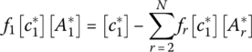
The effective viscoelastic properties are derived using the approach introduced by Dvorak and Benveniste (1992) along with the correspondence principle. For a macro‐scale homogeneous composite, a representative volume element (RVE) that contains N perfectly bonded phases can be selected. The volume averaged fields of the hybrid composite are given by:

(11.1)

and

(11.2)

where and denote the overall average stress and strain fields, respectively. Also, f_r denotes the volume fraction of phase r. Furthermore, and denote the average stress and strain fields in phase r, respectively.

The correspondence constitutive equation of the overall composite is given by

(11.3)

where [c^*] is the overall complex stiffness matrix in the principle material (1‐2‐3) coordinate system.

Similarly, the correspondence constitutive equation in each phase can be written as

(11.4)

where denotes the viscoelastic complex stiffness of phase r in the principle material coordinate system.

It has been shown that the overall average stress of the hybrid composite is given by (Dvorak and Benveniste 1992). Similarly, the overall average strain of the hybrid composite is given by . Thus, under uniform far field [ε⁰] or [σ⁰] the volume‐averages fields in phase r can be expressed as

(11.5)

and

(11.6)

where and are the correspondence concentration factors of phase r.

Substituting Eq. (11.1) into Eq. (11.5) and Eq. (11.2) into Eq. (11.6), yields:

(11.7)

and

(11.8)

Hence, Eqs. (11.7) and (11.8) yield the following expression:

(11.9)

where [I] denotes the identity matrix.

Combining Eqs. (11.4) and (11.5), gives:

(11.10)

Substituting Eq. (11.10) into Eq. (11.2), yields:

(11.11)

Comparing Eqs. (11.3) and (11.11), yields:

or

(11.12)

Using Eq. (11.9) yields:

or

i.e.

(11.13)

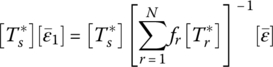
Substituting Eq. (11.13) into Eq. (11.13), gives the following expression for the overall viscoelastic stiffness and compliance in the principle material coordinate system:

(11.14)

In a similar manner, the corresponding expression for the overall viscoelastic compliance [s^*] in the principle material coordinate system is given by:

(11.15)

where and denote the complex stiffness and compliance of the matrix, respectively. Note that Eqs. (11.14) and (11.15) satisfy the internal consistency relationships; that is, the effective stiffness [c^*] and compliance [s^*] are the inverse of each other.

The correspondence concentration factors, and , can be estimated by the various micromechanics tools such as the Eshelby's method, the self‐consistent method, and the Mori–Tanaka approach, and so on. Among all those, the Mori–Tanaka approach is known to be one of the most elegant and accurate methods that can be used to estimate the overall elastic properties of aligned as well as randomly oriented short fiber composite (Tucker III and Liang 1999; Tandon and Weng 1986). Moreover, the Mori–Tanaka approach yields identical results when either a uniform elastic strain [ε⁰] or a uniform stress [σ⁰] field is prescribed at the boundary of the composite.

Inside the matrix, the stress [σ₁] is given by the following expression:

(11.20)

However, within the inclusion the stress [σ_r] is given by the following expression:

(11.21)

According to Eshelby's approach, the constrained strain [ε^C] is uniquely related to the transformation strain [ε^T] such that:

(11.22)

where [S^*] is the “Eshelby tensor,” which is a function of the Poisson's ratio of the matrix and the shape and geometry of the inclusions.

Furthermore, Eshelby developed an equivalence theorem between the problems of homogeneous inclusion and an inhomogeneous inclusion of the same shape. Such an equivalence can best be understood by considering the bodies shown in Figure 11.6a,b for the homogeneous and inhomogeneous inclusions, respectively. These inclusions have stiffnesses and , respectively.

In Figure 11.6a, the homogeneous inclusion is subjected to a transformation strain [ε^T] whereas the inhomogeneous inclusion of Figure 11.6b has no transformation strain. The two bodies of Figure 11.6 are subject to a uniform applied strain [ε^A]. Eshelby developed an expression for the transformation strain [ε^T] that results in the same stress and strain distributions in both problems. Hence, the constitutive Eq. (11.21) for the homogeneous inclusion can be modified to account for the applied strain [ε^A] to yield:

(11.23)

Accordingly, the corresponding constitutive equation for the inhomogeneous inclusion can be written as follows:

(11.24)

The equivalence of the stresses between the two problems yields:

(11.25)

Substituting Eq. (11.22) into Eq. (11.25) gives the following expression:

(11.26)

Equation (11.26) gives the expression of the transformation strain [ε^T] which is necessary for the equivalence in terms of the applied strain transformation strain [ε^A].

Note that, in the far field, the average strains in the matrix and the rth inclusion can be written as:

(11.27)

and

(11.28)

Then, substituting Eq. (11.28) into Eq. (11.25), it reduces to:

or

that is,

Hence,

(11.29)

Combining Eqs. (11.22) and (11.29) yields:

(11.30)

Substituting Eqs. (11.27) and (11.28) into Eq. (11.30), it reduces to:

or

(11.31)

In the Mori–Tanaka assumption, it is assumed that when many identical particles (inclusions) are embedded into the composite, the average particle strain is given by:

(11.32)

that is, each particle experiences a far‐field strain that is equal to the average strain of the matrix. In other words, a direct comparison between Eqs. (11.31) and (11.32) gives the following expression of the strain concentration factor:

(11.33)

This completes the proof of Eq. (11.18).

Now for proving Eq. (11.16), two approaches can be adopted:

First Approach:

This approach is simple and aiming at showing that the two sides of the equation are equal. It begins by multiplying both sides by f_s and summing up over the number of phases s = 1,…N inside the composite to yield the following:

(11.34)

that is, the right hand side of Eq. (11.34) is equal to an identity [I].

But, from Eq. (11.9), it is also seen that the left‐hand side of Eq. (11.34) is also equal to an identity I. Hence, Eq. (11.16) is valid.

Second Approach:

From Eq. (11.1), as:

Then, substituting Eq. (11.32) in this equation, yields:

(11.35)

Pre‐multiplying both sides by and using Eq. (11.32) gives the following expression:

(11.36)

From Eqs. (11.32) and (11.5), Eq. (11.36) reduces to:

Note that the Eshelby tensors for spheroidal inclusions, in an isotopic matrix, can be expressed as follows (Nemat‐Nasser and Hori 1999)

(11.37)

The elements of the Eshelby tensor are a function of the inclusion aspect ratio α = a₃/a₁ and the Poisson's ratio ν_m of the matrix as tabulated in Table 11.1. where g₁ and g₂ appearing in the table are defined as follows:

(11.38)

and

(11.39)

Shape	Thin disc (α = 0)	Sphere (α = 1)	Fiber (α → ∞)	Oblate spheroid (0 < α < 1, g = g1) and	Prolate spheroid (1 < α <  ∞ , g = g2)
S1111	0
S1122	0
S1133	0
S3311			0
S3333	1		0
S1313
S1212	0

11.2.2 Arbitrarily Oriented Inclusion Composites

Two processes are needed to find the effective properties of a hybrid composite with any desired inclusion orientation distribution. The first process is the evaluation of the effective properties for the hybrid composite with unidirectional aligned inclusions. This step is carried out in the previous section. The second process involves averaging the properties obtained from the first process in terms of the orientation distribution. Advani and Tucker III (1987) suggested a straightforward scheme for orientation averaging in short fiber composites. Furthermore, their averaging scheme can deliver reliable and accurate predictions for thermoelastic properties (Gusev et al. 2002). According to the approach of Advani and Tucker III (1987), the orientation average of Γ(θ, ϕ) is denoted by 〈Γ〉 and is defined as follows:

(11.40)

where ϕ and θ denote the two Euler angles that are usually used to describe the spatial orientation of an inclusion as shown in Figure 11.7. The angles (θ_i, ϕ_i) and (θ_f, ϕ_f) denote the lower and upper limits, respectively.

The inclusion distribution region is defined by (−θ₀ = θ_i) ≤ θ ≤ (θ_f = θ₀) and (π/2 − ϕ₀ = ϕ_i) ≤ ϕ ≤ (ϕ_f = π/2 + ϕ₀), where θ₀ and ϕ₀ are prescribed angles. The symbol, Ψ(θ, ϕ), denotes the probability distribution function. This function must satisfy specific conditions leading to:

(11.41)

Using Eq. (11.41) into Eq. (11.40) yields the final expression of the orientation average:

(11.42)

In this equation, the function Γ(θ, ϕ) can be used to represent the transformed viscoelastic stiffness, compliance, or any other property tensor in the global (1′‐2′‐3′) coordinate system. An expression for the transformed viscoelastic stiffness, , is determined by employing the transformation (Wetherhold 1988):

(11.43)

Similarly, the transformed viscoelastic compliance obtained by

(11.44)

where the transformation matrices [R₁] and [R₂] are defined in Appendix 11.A, and superscript T denotes the transpose.

Substituting Eqs. (11.43) and (11.44) into Eq. (11.42), one obtains the orientation average of the viscoelastic stiffness:

(11.45)

and the viscoelastic compliance:

(11.46)

Expressions (11.45) and (11.46) do not guarantee satisfying the internal consistency relationships. In other words, the orientation averaged stiffness (11.45) and compliance (11.46) are not necessarily each other’s inverse for all orientation distribution.

For predictions of the elastic properties, Hine et al. (2002, 2004) have shown that the orientation averaged stiffness and compliance equations, which are similar to (11.45) and (11.46), provide significantly different results for the thermoelastic properties of short fiber composites. Furthermore, Hine and coworkers have demonstrated that the stiffness equation provides accurate predictions of the orientation averaged properties when compared with the results from their numerical simulation.

According to this discussion, Eq. (11.45) will be used to explicitly determine the orientation averaged viscoelastic properties of the hybrid composites. Furthermore, the viscoelastic properties will be determined by evaluating the limits of Eq. (11.45) as the angles θ₀ and ϕ₀ approach certain values. Three general orientations will be considered. In aligned orientations, all the inclusions are uni‐directionally aligned along the 1′‐axis. To achieve this case, the values of θ₀ and ϕ₀ are set to approach zero. In two‐dimensional random orientations, the inclusions are randomly oriented in the 1′‐2′ plane. Here, the values of θ₀ and ϕ₀ are set to approach π and zero, respectively. In three‐dimensional random orientations, the inclusions are randomly oriented in all directions. In this orientation, the values of θ₀ and ϕ₀ are set to approach π and π/2, respectively. For these three orientations, the viscoelastic stiffness tensor can be written as:

(11.47)

where the components of are listed in Table 11.2.

	Aligned orientation (θ0 → 0, ϕ0 → 0)	2D random orientation (θ0 → π,  ϕ0 → 0)	3D random orientation (θ0 → π, ϕ0 → π/2)

Several properties can be extracted from the three‐dimensional moduli of the hybrid composite (11.47). For example, the complex modulus in the global coordinate system can be expressed as

(11.48)

and the loss factor is accordingly defined as

(11.49)

with modulus related to the compliance via the following expression:

(11.50)

and

(11.51)

where denotes the storage modulus, denotes the loss modulus, and subscript q denotes the contracted index.

Based on the theory presented in Section 11.2, the computation of the viscoelastic properties of particle‐filled polymer composites is carried out according to the flow chart displayed in Figure 11.8.

Table 11.3 lists the material properties of typical nanoparticles which are commonly used in manufacturing nanoparticle polymer composites.

Property	Particle
	PZT‐5Ha	PCM51b	MWCNTc	CBd	DGEBA‐DDMe	Hercules 3501‐6f
	127.2	129.22	999.66	9.2885	2.4409	7.4879
	80.2	86.4	369.74	3.9808	1.6962	4.5894
	84.67	83.06	369.74	3.9808	1.6962	4.5894
	117.44	116.9	999.66	9.2885	2.4409	7.4879
	23	28.83	314.96	2.6538	0.3723	1.4493
	23.5	21.41	314.96	2.6538	0.3723	1.4493
k31	0.388	0.37
k33	0.752	0.72
k15	0.675	0.72
ηm	–	–			0.047	0.03

^a Electro Ceramic Division, Morgan Matroc Inc., Bedford, OH.

^b Noliac, http://www.noliac.com (PCM51 is also called NCE51).

^c Tian and Wang (2008).

^d Aldraihem et al. (2007).

^e Pascault et al. (2002).

^f Lesieutre et al. (1993).

Solution

The isotropic stiffness matrix for the HDPE polymer is given by:

where , , , , , , , and .

Note that where E^*= complex modulus of HDPE, storage modulus, and η₁= loss factor. Values of and η₁ are displayed in Figure 11.5 as a function of frequency ω.

Similarly, for the CB nanoparticles, the stiffness matrix of the second phase of the composite is given by:

Note that is a matrix with real elements.

Figure 11.10 displays the values of the complex modulus of the CB‐filled HDPE polymer composite as predicted by the micromechanics approach outlined in Section 11.2 for CB volume fractions varying between 0 and 20%. These predictions are in excellent agreement with the corresponding experimental results shown in Figure 11.11.

It is important to note that plotting the storage modulus against the loss modulus results in a unified master line on which the characteristics of the CB/HDPE composite collapse for all the considered CB volume fractions. The equation of this line is:

The equation is valid for both the experimental results and micromechanics predictions. This leads to a loss factor η ≅1.

Furthermore, the displayed results indicate that increasing the CB concentration makes the composite stiffer, but at the expense of reducing its damping behavior as quantified by its loss factor.

Solution

Consider the Voigt and Reuss composites shown in Figure 11.12. Let and denote the stiffness tensors of the HDPE and CB, respectively. These tensors are as described in Example 11.1.

Then, the effective stiffness tensor of the Voigt model, which assumes the uniformity of the strain is given by:

(11.52)

where f₁ and f₂ are the volume fractions of HDPE and CB such that f₁ + f₂ = 1.

Similarly, the effective compliance tensor of the Reuss model, which assumes the uniformity of the stress is given by:

(11.53)

where and are the compliances of HDPE and CB.

Hence, the effective stiffness tensor of the Reuss model is given by:

(11.54)

Using Eqs. (11.52) through (11.54) yields the characteristics displayed in Figure 11.13 for frequencies of 0.01, 1, and 100 Hz. It can be seen that the viscoelastic characteristics of the CB/HDPE composite lie inside the Voigt and Reuss bounds.

Solution

Figures 11.16 and 11.17 show the E^′ − v characteristics and the Cole–Cole plot of E^′ versus E^″ following the use of the Smallwood–Guth Eq. (11.55). It can be seen that the equation results in collapsing the E^′ − v and E^′ − E^″ characteristics to form nearly single lines especially for CB volume fractions that are less than or equal to 15%.

These figures also display comparisons with the predictions obtained by using Eshelby's strain tensor approach. Close agreement is obvious between the predictions of the two approaches particularly for volume fractions less than 15%.

Solution

Figure 11.19a shows a finite element model of the RVE that is developed in ANSYS using SOLID186 elements. Figure 11.19b shows a unit cell with the associated boundary conditions that is used in analysis in order to simplify the computational effort (Brinson and Lin 1998).

Figure 11.20 displays a comparison between the deflections w in the z direction as predicted by Smallwood (1944) reinforcement theory and the ANSYS finite element of the RVE for a CB/polymer composite with a CB volume fraction of 20%. The Smallwood prediction is based on Eq. (11.B.9) given in the Appendix 11.B. The figures indicate that the contours of the deflection v as predicted by Smallwood model are in close agreement with those predicted by the ANSYS model.

Figure 11.21 displays the contours of the strain and stress, along the y direction, as predicted by the ANSYS finite element of an RVE of the CB/polymer composite with a CB volume fraction of 20%.

Figure 11.22 displays the contours of the deflection, along the z direction, as predicted by the ANSYS finite element of a RVE of the CB/polymer composite with a CB volume fraction ranging from 0 to 16.6%.

The effect of the volume fraction of the filler on the mechanical properties of a CB/polymer composite is determined using the approach outlined by Barbero (2013). In that approach, the components of the stiffness matrix c_αβ are determined by using the average stress and average strain such that:

(11.56)

where α and β = 1,…,6.

In Eq. (11.56), the average stresses are evaluated by computing the stress field over the entire RVE when a unit strain ε_β is applied along the β direction such that:

(11.57)

where V is the volume of the VRE.

The modulus of elasticity E_T and Poisson's ratio v_T in the transverse directions (y and z) are extracted from (Barbero 2013) as follows:

(11.58)

and

(11.59)

Figure 11.23 displays comparisons between the effect of the filler volume fraction on the reinforcement, in the z direction, as predicted by the ANSYS Finite Element, Smallwood–Guth model, and Eshelby's method. The reinforcement effect is quantified by the dimensionless ratio of the elastic modulus E_z of the CB/polymer composite, in the z direction, relative to the storage modulus of the pristine polymer E₀; that is, E_z/E₀.

The figure suggests that the Smallwood–Guth model adequately predicts the reinforcement effect over a practical range of filler volume fraction. Such a prediction is also computationally simple and efficient when compared to the finite element method (FEM) and Eshelby's method.

11.4.1 Basic Physical Characteristics

CB/polymer composites have attracted the attention for several decades primarily because of for their important use in manufacturing automotive tires. But, in this section, the emphasis is placed on their novel utilization in vibration damping applications. These applications stem mainly from of the fact that embedding CB inside the polymer matrix renders it to be electrically conducting. The extent of the electrical conduction depends on the volume fraction of the CB filler into the composite.

An important metric that quantifies the conductivity of the polymer is the “Percolation Threshold.” This threshold defines the concentration of the fillers that makes the polymer conductive. Generally speaking, as the concentration of the CB increases, the conductivity of the composite increases or the resistivity decreases as shown in Figure 11.24.

The figure indicates that the rate of increase of the conductivity, or decrease of resistivity, is slow at low concentrations as shown in region A of Figure 11.24. The resistivity drops rapidly with further increase in the CB as it goes into region B where the rate of change increases by more than 10 orders of magnitude. Further increase of the CB content fails to improve the resistivity as seen during region C.

It is important to physically understand the underlying phenomena that are behind such changes in the conductivity of the polymer matrix. At low CB content, the gap between the CB particles, where the electrons are transmitted, is very large and the resistivity of the composite is approximately that of the polymer matrix. As the concentration increases, the percolation threshold is reached where the resistivity starts to decrease abruptly as a function of the CB loading. In this region, region B, the gap between the CB particles is close but not touching. As a result, the electron must overcome the potential barrier and cross the gap between the CB particles.

In region C, where the CB loading is higher than the percolation threshold, the CB particles form chains that act as pure resistive conduits for conducting electricity as indicated in Figure 11.25. Figure 11.25a displays a schematic drawing of the microstructure of a CB/polymer composite whereas Figure 11.25b shows a scanning electron microscope photograph of the microstructure emphasizing the existence of CB chains.

Ding et al. (2013) and Wang et al. (2005) suggested that the equivalent electrical circuits of the CB/polymer composite depend, in general, on the CB volume fraction and, in particular, on the percolation characteristics as shown in Figure 11.26. In the figure, R_a, R_c, C_c, and L denote the CB aggregate resistance, the contact resistance, the contact capacitance, and inductance, respectively.

The full practical potential of the CB/polymer composites is usually utilized when operating in the first part of zone C where the transmission of electricity is governed primarily by the ohmic mechanism (R_a). Further increase of the CB content makes the mixing and manufacturing of a uniform CB composite rather difficult. More importantly, the complexity of the resulting equivalent electrical circuit of the composites complicates their operation.

For practical considerations, the contact capacitance and inductance are usually very small as reported by Wang et al. (2005). Therefore, the emphasis is placed here only on modeling the CB/polymer composites as resistive elements.

11.4.2 Modeling of the Piezo‐Resistance of CB/Polymer Composites

The electrical resistance R, under no loading conditions, of CB/Polymer composites can be determined from:

(11.60)

where ρ_s, A, and l_c denote the resistivity, cross sectional area, and thickness of the composite, respectively.

It is important to note that the electrical resistance of the composite is usually called “piezo‐resistance.” Such a resistance defines changes in the resistance of the CB/polymers due to the application of load.

Generally, the piezo‐resistance depends on the properties of the polymer matrix, filler properties and filler concentration, and applied load. An excellent account that describes the interactions between all these parameters and their effect on the piezo‐resistivity of the conducting polymer composite is given by Zhang et al. (2000, 2001). In their work, Zhang et al. developed a physics‐based mathematical model to predict the piezo‐resistivity of polymers impregnated with 11 different fillers.

The total resistance R of one conducting path is given by:

(11.61)

where R_c = resistance between two adjacent filler particles, R_a = resistance across filler particle, L = number of particles forming one path, and S = number of conducting paths.

If the inter‐particle separation is very large, no current flows. However, as the separation becomes adequately small, a tunneling current I will flow due to the application of a voltage V such that (Simmons 1963):

(11.62)

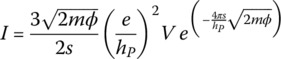
where m = electron mass, e = electron charge, h_P = Planck constant, s = separation between two adjacent particles, and ϕ = height of potential barrier between adjacent particles.

Assuming a² = the cross sectional area of the conducting particle, then the resistance R_c can be determined from:

(11.63)

where

(11.64)

Because the conductivity of the particles is very large compared with that between two adjacent particles, then R_a ≅ 0, reducing Eq. (11.61) to:

(11.65)

Equation (11.65) can be used to predict the resistance of the conducting polymer composite and it is clear that it varies exponentially with the separation distance s between the particles, which is a function of the applied load or strain experienced by the composite. Now, let us assume that the inter‐particle separation changes from s₀ to s due to the application of stress, then the fractional resistance change (−ΔR/R₀) can be predicted from:

(11.66)

where R₀ is the original resistance. Note that s and s₀ can be related to the strain ε and the stress σ by the following relationships:

(11.67)

where E = modulus of elasticity of the polymer matrix.

The initial separation distance s₀ is estimated from Han and Choi (1998) as follows:

(11.68)

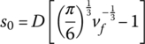
where D = particle diameter and v_f = volume fraction of filler.

Accordingly, Eq. (11.66) reduces to:

(11.69)

Equation (11.69) predicts the piezo‐resistance changes of conducting polymer composite as function of the applied stress σ, modulus of elasticity of the polymer matrix E, filler particle diameter D, filler volume fraction v, and the parameter γ. Equation (11.69) can be rewritten as:or

(11.70)

where

(11.71)

For σ/E < 0.01, Eq. (11.71) can be simplified to:

(11.72)

Expanding the exponential in Eq. (11.72), yields:

or

(11.73)

where R_ε is the resistance of the CB/polymer composites following the application of a strain ε. Equation (11.73) indicates that the relationship between R_ε/R₀ and the σ/E (or ε) is a straight line with a slope of as shown in Figure 11.27.

The value of can be determined, for CB particle‐filled polymer, using the following parameters: mass of the electron m = 9.180938E‐31 kg, h_P = Planck constant = 6.626E‐34 m² kg s⁻¹, and ϕ = 0.05 EV.

These parameters yield a slope of the piezo‐resistive characteristics of 54.97.

11.4.3 The Piezo‐Resistivity of CB/Polymer Composites

The electrical resistivity ρ_s of the CB/polymer composites can be determined by rewriting Eq. (11.65) as follows:

(11.74)

In Eq. (11.74), it is assumed that Sa² and LD denote the area and the length of the conducting path, respectively.

Figure 11.28 displays the resistivity of the CB/polymer composite as predicted by Eq. (11.74), with CB particles of an average size of 30 nm (Kaiser 1993), in comparison with the prediction of Schwartz et al. (2000). In their prediction approach, Schwartz et al. determined the electrical resistivity of a composite of CB in an insulating matrix in terms of the volume fraction of the CB and aggregate size and distribution. It is assumed that the resistance of a random lattice composite between sites different aggregates varies exponentially with the gap.

11.5.1 Finite Element Model

In this section, the CB/polymer is utilized as a means for vibration damping. Consider a rod consisting of an assembly of CB/polymer layers sandwiching, in a periodic manner, piezoelectric layers as shown in Figure 11.29.

The interaction between the dynamics of the piezoelectric layer that is shunted by the resistive CB/polymer layer is described using the constitutive equation of the piezo‐layer as given in Chapter 9 as follows:

(11.75)

where T₃ and S_3p are the stress and strain along the composite rod. Also, E₃ and D₃ denote the electric field and the electrical displacement, respectively. Furthermore, , , , and .

This form of constitutive relationship is used to generate the potential and kinetic energies of an element of the CB/polymer composite and shunted piezo‐network in terms of the DOF {Δ^e} = {u_i  u_j  u_k}^T and the electrical DOF Q^e (the charge of the eth cell). Note that the longitudinal displacements of the composite u_c (x) and piezo‐layer u_p (x), at any position x, are given by the following shape function

(11.76)

where {N_c} = {(1−x/l_c) x/l_c 0} and {N_p} = {0 (1−x/l_p) x/l_p} where l_c and l_p are equal the length of the composite layer and the piezo‐layer, respectively.

The kinetic energy KE of the eth unit cell can now be determined from:

(11.77)

where

• = mass matrix of the piezo‐layer,
• = mass matrix of the CB/polymer layer,
• and [M^e] = [M_p] + [M_c] = total mass of the eth unit cell.

Also, ρ_l and A_l denote the density and cross sectional area of the lth layer (l = p for the piezo‐layer and l = c for the CB/polymer layer, respectively).

The potential energy PE of the eth unit cell is given by:

(11.78)

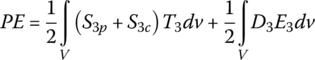
where S_3p = strain in the piezo‐layer = u_,xp, = stress on piezo‐layer, S_3c = strain in the CB/polymer layer = u_,xc, and = stress on CB/polymer layer with denoting the complex modulus of the composite layer.

Substituting from Eq. (11.75) into Eq. (11.78) gives:

(11.79)

Note that: S_3p = u_,xp = {N_,xp}{Δ^e}, S_3c = u_,xc = {N_,xc}{Δ^e}, and D₃ = Q^e/A_p = constant along the piezo‐layer, then Eq. (11.79) reduces to

(11.80)

where = stiffness matrix of piezo‐layer and CB/polymer assembly.

The virtual work δW associated with the inductive‐resistive‐capacitive shunting network of the CB/polymer composite and the external load {F_i} is given by:

(11.81)

Now, the equations governing the dynamics of the/piezo‐patch system can be extracted using the Lagrangian dynamics to give

and

(11.82)

where L_e, R_e, and C_e are the components of the inductive‐resistive‐capacitive shunting network of the CB/Polymer composite. Note that R_e = R_ε where it is assumed here that the effect of the strain on the resistance of the CB/Polymer composite is negligible, that is, R_e = R_ε ≈ R₀. This assumption is considered only to simplify the analysis and makes the finite element model linear to enable direct solution. But, when the resistance R_ε ≠ R₀, the analysis becomes iterative in nature and requires checking of the convergence at every time or frequency step.

These equations can be written in the following matrix form:

(11.83)

or

(11.84)

where , , ,

(11.85)

The equation of motion of the entire CB composite/shunted piezo‐network assembly can then be determined by assembling the mass and stiffness matrices of the individual cells to yield:

(11.86)

where [M_o], [C_o],   and [K_o] are the overall mass, damping, and stiffness matrices of the entire assembly. Also, {X} and {F_o} denote the structural and electrical DOF as well as load vectors of the entire assembly.

Note that bonding the shunted piezo‐layer to the CB composite has resulted in adding damping to the assembly as quantified by the damping matrix [C_o]. It has also modified the stiffness and mass matrices.

11.5.2 Condensed Model of a Unit Cell

As the CB/polymer composite can be treated electrically as a resistive element, then L_e and C_e are set equal to zero in Eq. (11.81). Further, using the static condensation method to condense the DOF of the charge Q^e leads to:

(11.87)

i.e. then:

(11.88)

Let e = {0 1  − 1}, then is given by:

(11.89)

Substituting Eq. (11.88) into Eq. (11.83) and pre‐multiplying by gives:

or

(11.90)

where and .

For the unit cell, shown in Figure 11.29, the nodal deflection vector {Δ^e} is defined as:

(11.91)

where u_k, u_j, and  u_i denote the bottom, internal, and top deflection vectors as shown in Figure 11.29b.

This vector is condensed to support the Bloch wave propagation (Hussein 2009). Hence, the displacements at the boundaries are related as follows:

(11.92)

where k and L denote the wave number and the length of the unit cell, respectively.

Hence, define an independent nodal deflection vector such that:

(11.93)

The deflection vectors {Δ^e} and are related as follows:

(11.94)

where is a transformation matrix such as:

(11.95)

Substituting Eqs. (11.94) and (11.95) into Eq. (11.90), it reduces to:

(11.96)

where , , , and .

Equation (11.95) is now cast in the following state‐space form (Meirovitch 2010):

(11.97)

where .

Let the state‐space solution be assumed as

(11.98)

where {Y}^c = { {x} + i{z}}^c and λ = iω.

Equation (11.98) reduces to the following eigenvalue problem:

(11.99)

In a compact form, Eq. (11.99) reduces to

(11.100)

where

(11.101)

Equating the real and imaginary coefficients on both sides of Eq. (11.100) yields:

(11.102)

(11.103)

Equations (11.102) and (11.103) can be rewritten in compact and standard eigenvalue problem form such that:

(11.104)

where [A]^c = [M^*]^c − 1 [ [D^*]^Tc[M^*]^c − 1[D^*]^c ].

Note that all the entries of the matrix [A]^c are functions of the dimensionless wave number kL. Therefore, the eigenvalues of the matrix [A]^c can be determined for different values of the wave number kL.

Then, the eigenvalues λ_s are given by

(11.105)

where s = 1 to n.

The dispersion characteristics of the unit cell are constructed by plotting the resonant frequency ω_s against the wave number kL. The resulted dispersion curves further define the zones of stop and pass bands of the cell as described in Chapter 10.

Solution

Figure 11.30 parts a–c displays the dispersion characteristics of the non‐conducting VEM, conducting VEM with R_e = 10 kohm, and VEM with R_e = 1 Mohm, respectively.

Comparing Figure 11.30a,b indicates that making the VEM layer conduct with the CB filler, with an effective resistance of R_e = 10 kohm, has resulted in enhancing the stop band characteristics, particularly at the high frequency end. Further increase of the effective resistance by adding an additional external resistance to augment the piezo‐resistance of the VEM conducting layer to reach 1 Mohm has significantly improved the stop band characteristics and extended it to 1 MHz as indicated in Figure 11.30c.

The effect of such improvements in the stop band characteristics is demonstrated clearly in the frequency response behavior of the composite as shown in Figure 11.31a,b.

Figure 11.31a indicates that the embedding the CB filler in the pristine VEM layer has introduced two important effects when the effective piezo‐resistance is R_e = 10 Kohm. The first effect appears in the form of the reinforcement of the polymer, as predicted by the reinforcement theory of Smallwood (1944), which has resulted in stiffening the VEM. Such a stiffening effect is manifested by the shift of the resonant frequencies to higher frequency ranges that, in turn, produced a significant attenuation of the transmitted vibration.

The second effect manifests itself by the vibration attenuation at high frequencies, particularly at 12.93 KHz, which is attributed to the energy dissipation due to shunting of the piezo‐layer by the piezo‐resistance of the conducting VEM/CB layer.

Increasing further the effective shunting resistance to R_e = 1 Mohm, as indicated in Figure 11.31b resulted in complete blockage of the high frequency vibration around 12 KHz. Such a blockage is due to the enhanced stop band characteristics shown in Figure 11.30c.

PROPERTY	Geometry		Piezo‐layer				Viscoelastic layer
	lc = lp (m)	Ac = Ap (m2)	sE(m2 N−1)	d33(m V−1)	k33	ρp (kg m−3)	Ev (N m−2)	α	ωn (rad s−1)	ζ	ρv (kg m−3)
VALUE	0.1	0.01	16 × 10−12	296 × 10−12	0.37	7600	1E4	5	25,000	10	1100

11.6.1 Composite Description and Assumptions

The hybrid composite considered in this section, shown in Figure 11.32, consists of a polymer matrix, electrically conducting particles, and piezoelectric inclusions. All the ingredients of the composite are assumed to be perfectly bonded. Further, the inclusions are assumed to be spheroidal in shapes that are arbitrarily oriented within the matrix. The considered piezoelectric inclusions are assumed to be transversely isotropic with poling directions and electrodes in the three direction. The state of stress and electrode distributions of all the piezoelectric inclusions are assumed identical and uniform. The electrically conducting particles and the matrix are assumed to form resistive electric current paths R, which are adequate to load the piezoelectric inclusions (Aldraihem 2011; Aldraihem et al. 2007) as displayed in Figure 11.32b. Finally, the composite is assumed to be homogeneous on the macro‐scale and obeys the basic assumptions used in micromechanics analysis.

11.6.2 Shunted Piezoelectric Inclusions

Consider a hybrid composite that is subjected to a far‐field stress in the composite global (1′‐2′‐3′) coordinate system. Then, each of the embedded piezoelectric inclusions generates an electric energy that is dissipated into the resistance of the surrounding conducting polymer matrix. As outlined in Chapter 9, a resistively shunted piezoelectric element behaves like a VEM with the nonzero compliances, in the principle material (1‐2‐3) coordinate system, which are defined as follows:

(11.106)

(11.107)

(11.108)

(11.109)

(11.110)

(11.111)

(11.112)

In Eqs. (11.106a)–(11.106f) and (11.107), denotes the elements of elastic compliance matrix at constant electric field. Also, k₃₁, k₃₃, and k₁₅ denote the piezoelectric coupling factors, is the dielectric permittivity at constant stress, R is the shunt resistance, and ω is the frequency. Furthermore, a₃ defines the inclusion half‐length and A is the electrodes area with normal along the three‐axis as shown in Figure 11.7.

For the considered shunting, Eqs. (11.106a)–(11.106f) indicates that the out‐of‐plane shear compliances exhibit open‐circuit conditions, the in‐plane shear compliance exhibits short‐circuit conditions, whereas the remaining compliances exhibit shunted‐circuit conditions. Hence, the shear compliances primarily behave in an elastic manner and have limited damping capacity.

Substituting Eq. (11.107) into Eqs. (11.106a)–(11.106f), yields the complex compliance matrix that can be separated into real and imaginary parts as follows:

(11.113)

where [s^′] and [s^″] denote the real and imaginary part of the compliance, respectively.

Equations (11.106a)–(11.106f) or (11.107) represent the compliances in the principle material (1‐2‐3) coordinate system. Moreover, the compliance can be used to extract the stiffness as the stiffness is inverse of the compliance; that is, [c^*] = [s^*]⁻¹ and [c^E] = [s^E]⁻¹.

11.6.3 Typical Performance Characteristics of Hybrid Composites

In this section, the micromechanics model presented in Section 11.6.2 is utilized to predict the mechanical properties of a hybrid composite consisting of an epoxy matrix (Hercules 3501‐6) (Lesieutre et al. 1993), CB particles, and piezoelectric particles (Noliac^® – PCM51). The physical properties of the three ingredients of the composite are listed in Table 11.3. The epoxy has a Poisson's ratio, v, of 0.38, and the CB particles are embedded with a volume fraction 0.20. It is assumed that the piezo‐particles have aligned orientations.

It should be mentioned that both the inclusions shape and shunting characteristics are unknown. Hence, in the model predictions the inclusions aspect ratio, α, and the shunt frequency, Ω, are investigated.

Figure 11.33a displays the damping ratios of the composite in direction 1 and 2, as function of the shunt frequency, Ω = R C^Tω for different values of the volume fraction v_p of the piezo‐particles and for aspect ratio α = 100. The figures indicate that there are optimal values of ohm, that is, optimal shunting resistance, for each volume fractions v_p at which the loss factor attain maximum values. It can be seen that these values of ohm are 1.68, 1.54, and 1.43 when the volume fractions v_p are equal to 0.15, 0.35, and 0.55. The corresponding maximum loss factors are 9.67, 11.45, and 11.99, respectively. The values of the loss factors are normalized with respect to that of the epoxy matrix. This indicates that using the shunting of the piezo‐particles enhances the damping characteristics by almost an order of magnitude in both the one and two directions as the hybrid composite is transversally isotropic.

In direction 3, that is, during compression loading, the corresponding maximum loss factors are 0.81, 0.68, and 0.67 when the volume fractions v_p are equal to 0.15, 0.35, and 0.55, respectively, as shown in Figure 11.33b. The corresponding optimal shunt frequencies ohm are 1.28, 1.17, and 1.035.

Figures 11.34 and 11.35 display the effects of the volume fraction of the piezo‐particles v_p and aspect ratio α, respectively. The figures indicate that increasing the volume fraction and the aspect ratio result in a significant increase in the transverse loss factor. The opposite is true for the compressive loss factors.

The displayed results in Figures 11.33" through 11.35 indicate that the loss factors of the hybrid composite depend on the volume fraction, the orientation distribution, the aspect ratio (shape), and the shunt frequency‐resistance parameter. Table 11.5 summarizes a listing of the shunt frequency parameter ohm at which the loss factor ratio, η/η_m, attains maximum values for different orientation distributions and various aspect ratios. The listed values are calculated for piezo‐particles PCM51 with volume fraction of 35% and CB volume fraction of 25%.

Inclusion aspect ratio (α)	Aligned orientation (θ0 → 0,  ϕ0 → 0)				2D random orientation (θ0 → π,   ϕ0 → 0)						3D random orientation (θ0 → π,   ϕ0 → π/2)
0.0	1.16	0.62	1.13	2.36	1.75	3.71	1.16	2.42	2.03	4.41	1.78	3.71	2.02	4.42
0.5	1.07	1.18	1.06	0.92	1.03	1.23	1.08	0.92	1.16	0.71	1.01	1.10	1.10	0.71
1.0	1.07	1.53	1.07	0.84	1.11	1.37	1.07	0.84	1.34	0.75	1.06	1.23	1.28	0.75
100	1.58	11.45	1.13	0.68	2.12	8.45	1.16	0.68	2.43	7.52	2.05	8.47	2.44	7.52
1000	1.59	11.61	1.19	0.68	2.15	8.60	1.16	0.68	2.49	7.68	2.02	8.47	2.51	7.68

Figures 11.36–11.38 display the effect of the shunt frequency, piezo‐particle volume fraction, and piezo‐particles aspect ratio on the compliance coefficients of the hybrid composite, respectively.

The transformation matrix shown in Eqs. (11.43) and (11.44) is defined by Wetherhold (1988):

(11.A.1)

with

(11.A.2)

where θ and φ are rotation Euler angles defined in Figure 11.3.

The transformation matrix [R₂] shown in Eqs. (11.43) and (11.44) can be obtained by the relationship:

(11.A.3)

11.B.1 Basics

In this appendix, the reinforcement of a polymer by virtue of embedding solid particles in it is analyzed using the approach developed by Smallwood (1944) in an attempt to determine the effect of particle size and volume fraction on the modulus of the resulting composite.

Consider a rigid, spherical filler particle of radius R embedded in an isotropic polymer of known storage modulus as shown in Figure 11.B.1. The deflections and the resulting stresses near the particle are determined when the polymer is subjected to unidirectional tensile force T along the y direction.

The governing equilibrium equations as obtained from the theory of elasticity are given, for example by Barber (2010), as follows:

(11.B.1)

where u, v, w are the deflections along the x, y, z directions. Also, Δ denotes the cubical dilation (Δ = ε_xx + ε_yy + ε_zz) and ∇ is the Laplacian. Note that the equilibrium Eq. (11.B.1) are written in terms of the Lamé constants λ and μ that are related to Young's modulus E and Poisson's ratio, υ, such that (Reddy 2013):

(11.B.2)

Note that Lamé constants λ and μ are also given by:

(11.B.3)

where G is the shear modulus.

Equation (11.B.1) are subjected to the following boundary conditions:

(11.B.4)

(11.B.5)

(11.B.6)

and

(11.B.7)

The boundary conditions given by Eqs. (11.B.4) through (11.B.7), at r = ∞, indicate that far away from the particle, the deflections (u, v, w) are caused only by the tension T.

Solutions of Eq. (11.B.1) subject to the boundary conditions are as follows:

(11.B.8)

(11.B.9)

and

(11.B.10)

where , r² = x² + y² + z², and

Assuming that Poisson's ratio μ of the composite is close to that of the polymer, which is nearly 0.5. Eq. (11.B.2) can be rewritten as:

(11.B.11)

For such a limit (μ/λ ≅ 0), the parameters A, B, and C reduce to:

(11.B.12)

In order to quantify the effect of the filler particle, the strain energy function W_T is determined as follows:

(11.B.13)

where N is the number of particles and V is the total volume of the polymer and the particles.

Then, the strain energy per unit volume is given by:

(11.B.14)

where v is the volume fraction of the particles.

Substituting Eqs. (11.B.3) and (11.B.12) into Eq. (11.B.14) yields:

(11.B.15)

The deflection w, at any point, due to the effect of all the filler particles is given by modifying Eq. (11.B.7) to take the following form:

(11.B.16)

where accounts for the effect of the particles and takes the following form (Smallwood 1944):

(11.B.17)

Then, the associated strain energy per unit volume is given by:

(11.B.18)

The equivalence of Eqs. (11.B.15) and (11.B.18) yields:

(11.B.19)

Expanding Eq. (11.B.19) into a first order Taylor series yields:

(11.B.20)

Song and Zheng (2016) summarized a list of other mathematical models that intend to improve the approximation of Smallwood Eq. (11.B.20) by adding higher order terms. In their summary, the coefficient of second order Taylor series expansion v² is reported by to vary between 2.5 and 15.6 depending on the adopted mathematical model. In here, the approach developed by Smallwood (1944) and then modified by Guth (1945) yields the following commonly used reinforcement relationship:

(11.B.21)

References

- Advani, S.G. and Tucker, C.L. III (1987). The use of tensors to describe and predict fiber orientation in short fiber composites. Journal of Rheology 31: 751–784.
- Aldraihem, O.J. (2011). Micromechanics modeling of viscoelastic properties of hybrid composites with shunted and arbitrarily oriented piezoelectric inclusions. Mechanics of Materials 43: 740–753.
- Aldraihem, O.J., Baz, A., and Al‐Saud, T.S. (2007). Hybrid composites with shunted piezoelectric particles for vibration damping. Mechanics of Advanced Materials and Structures 14: 413–426.
- ANSI/IEEE Std 176‐1987 (1987)., Standards Committee of the IEEE Ultrasonic, Ferroelectrics, and Frequency Control Society, American National Standard IEEE Standard on Piezoelectricity, Institute of Electrical and Electronics Engineers, Inc., New York, USA, 1987.
- Barber, J. R. (2010). Solid Mechanics and Its Applications, 3rd ed. Springer.
- Barbero, E.J. (2013). Finite Element Analysis of Composite Materials Using ANSYS®, 2e. CRC Press.
- Brinson, L.C. and Lin, W.S. (1998). Comparison of micromechanics methods for effective properties of multiphase viscoelastic composites. Composite Structures 41: 353–367.
- Ding, N., Wang, L., Zuo, P. et al. (2013). Study on electrical properties of activated carbon black filled polypropylene composites using impedance analyser. Advanced Materials Research 712–715: 175–181.
- Dvorak, G.J. and Benveniste, Y. (1992). On transformation strains and uniform fields in multiphase elastic media. Proceedings of the Royal Society: Mathematical and Physical Sciences 437: 291–310.
- Electro Ceramic Division. (n.d.) “Data for designers,” Morgan Matroc Inc., 232 Forbes Road, Bedford, OH 44146.
- Eshelby, J.D. (1957). The determination of elastic field of an ellipsoidal inclusion and related problems. Proceedings of Royal Society of London 276–396.
- Gonella, S. and Ruzzene, M. (2008). Homogenization of vibrating periodic lattice structures. Applied Mathematical Modelling 32 (4): 459–482.
- Gusev, A., Heggli, M., Lusti, H.R., and Hine, P.J. (2002). Orientation averaging for stiffness and thermal expansion of short fiber composites. Advanced Engineering Materials 4: 931–933.
- Guth, E.J. (1945). Theory of filler reinforcement. Journal of Applied of Physics 16: 20–25.
- Han, D.G. and Choi, G.M. (1998). Computer simulation of the electrical conductivity of composites: the effect of geometrical arrangement. Solid State Ionics 106: 71–87.
- Hashin, Z. and Shtrikman, S. (1962). On some variational principles in anisotropic and nonhomogeneous elasticity. Journal of the Mechanics and Physics of Solids 10: 335–342.
- Hine, P.J., Lusti, H.R., and Gusev, A. (2004). On the possibility of reduced variable predictions for the thermoelastic properties of short fiber composites. Composites Science and Technology 64: 1081–1088.
- Hine, P.J., Lusti, H.R., and Gusev, A.A. (2002). Numerical simulation of the effects of volume fraction, aspect ratio and fiber length distribution on the elastic and thermoelastic properties of short fiber composites. Composites Science and Technology 62: 1445–1453.
- Hussein, M.I. (2009). Theory of damped bloch waves in elastic media. Physical Reviews B 80: 212301.
- Kaiser, J.H. (1993). Microwave evaluation of the conductive filler particles of carbon black‐rubber composites. Applied Physics A 56: 299–302.
- Leblanc, J.L. (2002). Rubber–filler interactions and rheological properties in filled compounds. Progress in Polymer Science 27 (4): 627–687.
- Lesieutre, G.A., Yarlagadda, S., Yoshikawa, S. et al. (1993). Passively damped structural composite materials using resistively shunted piezoceramic fibers. Journal of Materials Engineering and Performance 2: 887–892.
- Marenić E., Brancherie D., and Bonnet M., “Multiscale asymptotic‐based modeling of local material inhomogeneities”, Proceedings of the 8th International Congress of Croatian Society of Mechanics, 29 September − 2 October 2015, Opatija, Croatia, 2015.
- Meirovitch, L. (2010). Fundamentals of Vibration. Long Grove, IL: Waveland.
- Mori, T. and Tanaka, K. (1973). Average stress in matrix and average elastic energy of materials with misfitting inclusion. Acta Metallurgica 21: 571–574.
- Nemat‐Nasser, S. and Hori, M. (1999). Micromechanics: Overall Properties of Heterogeneous Materials, Second Revised Edition. Amsterdam: Elsevier.
- Noliac, Piezoelectric Particles: (2018)Available online at http://www.noliac.com (accessed June 2018).
- Pascault, J.P., Sauterau, H., Verdu, J., and Williams, R.J.J. (2002). Thermosetting Polymers. New York, NY: Marcel Dekker.
- Prasad J. and Diaz A. R. “A concept for a material that softens with frequency”, Paper No. DETC2007–34299, pp. 761–768, Proceedings of the ASME 2007 International Design Engineering Technical Conferences and Computers and Information in Engineering Conference, Vol. 6, 33rd Design Automation Conference, Las Vegas, NV, USA, September 4–7, 2007.
- Reddy, J.N. (2013). An Introduction to Continuum Mechanics. Cambridge University Press.
- Reuss, A. (1929). Berechnung der Fließgrenze von Mischkristallen auf Grund der Plastizitatsbedingung für Einkristalle. Zeitschrift für Angewandte Mathematik und Mechanik 9: 49–58.
- Schwartz, G., Cerveny, S., and Marzocca, A.J. (2000). A numerical simulation of the electrical resistivity of carbon black filled rubber. Polymer 41: 6589–6595.
- Sejnoha, M. and Zeman, J. (2013). Micromechanics in Practice. Southampton, UK: WIT Press.
- Simmons, J.G. (1963). Generalized formula for the electric tunnel effect between similar electrodes separated by a thin insulating film. Journal of Applied Physics 34 (6): 1793–1803.
- Smallwood, H.M. (1944). Limiting law of the reinforcement of rubber. Journal of Applied Physics 15: 758–766.
- Song, Y. and Zheng, Q. (2016). Concepts and conflicts in nanoparticles reinforcement to polymers beyond hydrodynamics. Progress in Materials Science 84: 1–58.
- Tandon, G.P. and Weng, G.J. (1986). Average stress in the matrix and effective moduli of randomly oriented composites. Composites Science and Technology 27: 111–132.
- Tian, S. and Wang, X. (2008). Fabrication and performances of epoxy/multi‐walled carbon nanotubes/piezoelectric ceramic composites as rigid piezo‐damping materials. Journal of Materials Science 43: 4979–4987.
- Torquato, S. (2001). Random Heterogeneous Materials: Microstructure and Macroscopic Properties. New York, NY: Springer.
- Tucker, C.L. III and Liang, E. (1999). Stiffness predictions for unidirectional short‐fiber composites: review and evaluation. Composites Science and Technology 59: 655–671.
- Voigt, W. (1887). Theorie des Lichts für bewegte Medien. Göttinger Nachrichten 8: 177–238.
- Wang, Y.‐J., Pan, Y., Zhang, X.‐W., and Tan, K. (2005). Impedance spectra of carbon black filled high‐density polyethylene composites. Journal of Applied Polymer Science 98: 1344–1350.
- Wetherhold, R.C. (1988). Elastic Plates Theory and Application, Riesmann, H. New York, NY: Wiley, Chapter 10.
- Zhang, J.F. and Yi, X.S. (2002). Dynamic rheological behavior of high‐density polyethylene filled with carbon black. Journal of Applied Polymer Science 86: 3527–3531.
- Zhang, X.W., Pan, Y., Zheng, Q., and Yi, X.S. (2000). Time dependence of piezoresistance for conductor‐filled polymer composites. Journal of Applied Polymer Science Part B: Polymer Physics 38: 2739–2749.
- Zhang, X.W., Pan, Y., Zheng, Q., and Yi, X.S. (2001). Piezoresistance of conductor filled insulator composites. Polymer International 50: 229–236.
11.A Transformation Matrix