The Method of Universal Generating Functions (U-functions), introduced by Ushakov (1986), actually represents a generalization of Kettelle's Algorithm. This method suggests a transparent and convenient method of computerized solutions of various enumeration problems, in particular, the optimal redundancy problem.

6.1 Generating Function

First, let us refresh our memory concerning generating functions. This is a very convenient tool widely used in probability theory for finding joint distributions of several discrete random variables. Generating function is defined as:

(6.1)

where p_k is the probability that discrete random variable X takes value k and G_k is the distribution function domain. In optimal redundancy problems, in principle, G_k = [0, ∞), though any practical task has its own limitations on the largest value of k.

Consider two non-negative discrete random values X₁ and X₂ with distributions

and

correspondingly, where n₁ and n₂ are numbers of discrete values of each type. For finding probability of random variable X = X⁽¹⁾ + X⁽²⁾, one should enumerate all possible pairs of X⁽¹⁾ and X⁽²⁾ that give in sum value k and add corresponding probabilities:

X⁽¹⁾ = 0, X⁽²⁾ = k, with probability ,

X⁽¹⁾ = 1, X⁽²⁾ = k − 1, with probability ,

X⁽¹⁾ = 2, X⁽²⁾ = k − 2, with probability ,

…

X⁽¹⁾ = k, X⁽²⁾ = 0, with probability .

Thus the probability of interest is equal to

(6.2)

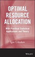
One can see that there is a convolution transform. It is clear that the same result will be obtained if one takes a polynomial

(6.3)

and, after combining like terms of expansions, finds the coefficient at z^k.

6.2 Universal GF (U-function)

One sees that algebraic argument “z” was introduced only for convenience: everybody knows that polynomial multiplication means products of coefficients and sums of powers. Such presentation helps one to obtain a distribution of the convolution of discrete random variables. However, what if random variables should be exposed to transformation different from convolution? For instance, if these random variables are arguments of some function?

Let us use habitual form of presentation, using symbol “⊗” instead of “П” just to underline that this is not an ordinary product of two GFs but a special transformation:

(6.4)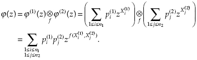

The subscript “f” in means that some specific operation f will be undertaken over values X. It is clear that in the case of “pure” GF function is operation of summation.

In the general case, using the polynomial form of GF is inconvenient and even impossible. In order to move further, let us introduce some terms. We previously said that a system consists of units that are physical objects characterized by their parameters: reliability, cost, weight, and so on. So we can consider each unit as a multiplet of its parameter. Reliability of each unit can be improved by using redundancy or by replacing units with more effective units. In other words, on a design stage an engineer deals with a “string” of possible multiplets characterizing various variants of a considered unit.

Consider a series system of two units. Unit 1 and Unit 2 are characterized by strings:

and

Each multiplet is a set of parameters where N is the number of parameters in each multiplet.

“Interaction” of these two strings is an analogue of the Cartesian product whose members fill the cells of Table 6.1.

TABLE 6.1 “Interaction” of Two Strings

Interaction of multiplets consists of interaction of their similar parameters, for instance,

(6.5)

Operator ⊗, as well as each operator , in most natural practical cases possesses the commutativity property, that is,

(6.6)

and the associativity property, that is,

(6.7)

Of course, operator depends on the physical nature of parameter α_s and the type of structure, that is, series or parallel (see Table 6.2).

TABLE 6.2 “Interaction” of Various Parameters for Series and Parallel Connections

Type of parameter	Type of structure	Result of interaction
(A) α is unit's PFFO (probability of failure-free operation)	Series
	Parallel
(B) α is number of units in parallel	Series
	Parallel
(C) α is unit's cost (weight)	Series
	Parallel
(D) α is unit's ohmic resistance	Series
	Parallel
(E) α is unit's capacitance	Series
	Parallel
(F) α is pipeline unit's capacitance	Series
	Parallel
(G) α is unit's random time to failure	Series
	Parallel

In the problem of optimal redundancy, one deals with triplet of type “Probability–Cost–Number of units” for each redundant group: M_j = {α_1j, α_2j, α_3j}. If there is a system of n series subsystems (single elements or redundant groups), one has to use a procedure almost completely coincided with the procedure of compiling the dominating sequences at Kettelle's algorithm. In other words, the problem reduces to constructing a single “equivalent unit” that possesses the entire system's properties. There are two possible ways of “convolving” the system into a single “equivalent unit”: dichotomous and sequential. We will demonstrate these two possible procedures in an example of a series system of four subsystems (see descriptions in Fig. 6.1 and Fig. 6.2).

FIGURE 6.1 Dichotomous scheme of compiling the equivalent unit.

FIGURE 6.2 Dichotomous scheme of compiling the equivalent unit.

Example 6.1

Consider a series system of four units with parameters as given in Table 6.3. Assume that “hot” redundancy of each unit is used for the system reliability improvement.

TABLE 6.3 System Unit Parameters

Let us solve two problems of optimal redundancy:

(a) Find the optimal allocation of redundant units to reach required PFFO level of 0.95.

(b) Find the optimal allocation of redundant units to reach maximum possible PFFO (probability of failure-free operation) level under the condition that the total cost of the system does not exceed 30 cost units.

In this case, each unit is characterized by the following strings of triplets (cost, PFFO, number):

S₁ = [{3; 0.6; 1}, …, {12; 0.9744; 4}, {15; 0.9898; 5}, {18; 0.9959; 6}, {21; 0.9984; 7}, {24; 0.9993; 8}, {27; 0.9997; 9}, …]

S₂ = [{1.5; 0.6; 1}, …, {6; 0.9744; 4}, {7.5; 0.9898; 5}, {9; 0.9959; 6}, {10.5; 0.9984; 7}, {12; 0.9993; 8}, {13.5; 0.9997; 9}, …]

S₃ = [{2; 0.7; 1}, …, {6; 0.9730; 3}, {8; 0.9919; 4}, {10; 0.9976; 5}, {12; 0.9993; 6}, {14; 0.9998; 7}, {16; 0.9999; 8}, …]

S₄ = [{1.2; 0.7; 1}, …, {3.6; 0.9730; 3}, {4.8; 0.9919; 4}, {6; 0.9976; 5}, {7.2; 0.9993; 6}, {8.4; 0.9998; 7}, {9.6; 0.9999; 8}, …].

Let us apply the dichotomous scheme of compiling equivalent units, and, first, consider the subsystem consisting of Unit 1 and Unit 2 (Table 6.4). We omit all intermediate calculations performed with the help of a simple Excel program.

TABLE 6.4 Triplets Belonging to

In Table 6.4, as well as in Tables 6.5 and 6.6, shaded entries indicate those triplets which are dominated. In the same manner, we construct (Table 6.5).

TABLE 6.5 Triplets Belonging to

TABLE 6.6 Resulting String of Triplets for the Equivalent Unit

Now on the basis of and , one constructs the final string for the equivalent unit. The result is given in the Table 6.6. One can notice that the final string in this particular case completely coincides with the final dominating sequence obtained by the Kettelle's Algorithm: the only difference is that we kept “the track of solving process” and have the resulting solution immediately from the table. (Frankly speaking, Kettele's Algorithm could be easily modified to get the same property of the final solution.)

Solutions of the problems above can be easily found from Table 6.6. The first time PFFO exceeds a level of 0.95 is when X = (4,5,5,4) and the corresponding system cost is 33.5 cost units. The second task has solution X = (4,4,5,3) with the cost equal to exactly 30 cost units. PFFO for this case is equal to 0.9216.

---

As the conclusion of this chapter, let us notice that the U-function method is very constructive not only for solving optimal redundancy problems, but also for a number of other problems, particularly those associated with multi-state systems analysis.

Chronological Bibliography

Ushakov, I. A. 1986. “A Universal Generating Function” (in Russian). Engineering Cybernetics, no. 5.

Ushakov, I. A. 1987. “Universal generating function.” Soviet Journal of Computer and System Science, no. 3.

Ushakov, I. A. 1987. “Optimal standby problem and a universal generating function.” Soviet Journal of Computer and System Science, no. 4.

Ushakov, I. A. 1987. “Solution of multi-criteria discrete optimization problems using a universal generating function.” Soviet Journal of Computer and System Sciences, no. 5.

Ushakov, I. A. 1988. “Solving of optimal redundancy problem by means of a generalized generating function.” Elektronische Informationsverarbeitung und Kybernetik, no. 4–5.

Ushakov, I. A. 2000. “The method of generating sequences.” European Journal of Operational Research, vol. 125, no. 2.

Levitin, G. 2005. The Universal Generating Function in Reliability Analysis and Optimisation. Springer-Verlag.

Chakravarty, S., and Ushakov, I. A. 2008. “Object Oriented Commonalities in Universal Generating Function for Reliability and in C++.” Reliability and Risk Analysis: Theory and Applications, no. 10.