Chapter 2

Spectrum Sensing: Basic Techniques

2.1 Challenges

Spectrum sensing in a cognitive radio is practically challenging, as shown in Table 2.2 [36, 37].

2.2 Energy Detection: No Prior Information about Deterministic or Stochastic Signal

Energy detection is the simplest spectrum sensing technique. It is a blind technique in that no prior information about the signal is required. It simply treats the primary signal as noise and decides on the presence or absence of the primary signal based on the energy of the observed signal. It does not involve complicated signal processing and has low complexity. In practice, energy detection is especially suitable for wideband spectrum sensing. The simultaneous sensing of multiple subbands can be realized by scanning the received wideband signal.

Two stages of sensing are desirable. The first stage uses the simplest energy detection. The second stage uses advanced techniques.

Table 2.1 Receiver parameters for 802.22 WRAN

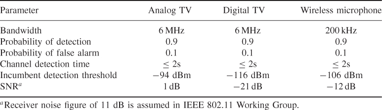
Table 2.2 Challenges for spectrum sensing

Practical challenges	Consequences	Comments
Very strict sensing requirements	See Table 2.1	To avoid “hidden node” problem
Unknown propagation channel and nonsynchronization	Make coherent detection unreliable	To relieve the primary user from the burden
Noise/interference uncertainty	Very difficult to estimate their power	Change with time and location

We follow [38] and [39–42] for the development below. Although the process is for band-pass, in general, one can still deal with its low-pass equivalent form and eventually translate it back to its band-pass type [43]. Besides, it has been verified [38] that both low-pass and band-pass processes are equivalent from the decision statistics perspective which is our main concern. Therefore, for convenience, we only address the problem for a low-pass process, following [41, 42].

2.2.1 Detection in White Noise: Lowpass Case

The detection is a test of the following hypotheses:

The output of the integrator is denoted by Y. We concentrate on a particular interval, say, (0, T), and take the test statistic as Y or any quantity monotonic with Y. We shall find it convenient to express the false alarm and detection probabilities using the related quantity

2.1

The choice of T as the sampling instant is a matter of convenience; any interval of duration will serve.

It is known that a sample function, of duration T, of a process which has a bandwidth W (negligible outside this band) is described approximately by a set of sample values 2TW in number. In the case of low-pass processes, the values are obtained by sampling the processes at times 1/2W apart. In the case of relatively narrowband band-pass process, the values are obtained from the in-phase and quadrature modulation components sampled at times 1/W apart.

With an appropriate choice of time origin, we may express each sample of noise as [44]

2.2

where sinc(x) = sinπx/πx, and

2.3

Clearly, each n_i is a Gaussian random variable with zero mean and with the same variance , which is the variance of n(t); that is,

2.4

Using the fact that

2.5

we may write

2.6

Over the interval (0, T), n(t) may be approximated by a finite sum of 2TW terms, as follows:

2.7

Similarly, the energy in a sample of duration T is approximated by 2TW terms of the right side of (2.6):

2.8

More rigor can be achieved by using the Karhunen-Loeve expansion (also called transform). Equation (2.8) may be considered as an approximation, valid for large T, after substituting (2.7) into the left-hand side of (2.8), or by using (2.39) and the statement in Section 2.2.5 to justify taking only 2TW terms of (2.6).

We can see that (2.8) is , with here being the test statistic under hypothesis . Let us write

2.9

2.10

Thus, is the sum of the squares of 2TW Gaussian random variables, each with zero mean and unit variance. is said to have a chi-square distribution with 2TW degrees of freedom, for which extensive tables exist [45–47].

Now consider the case where the input y(t) has the signal s(t) present. The segment of signal duration T may be represented by a finite sum of 2TW terms,

2.11

where

2.12

By following the reasoning above, we can approximate the signal energy in the interval (0, T) by

2.13

Define the coefficients by

2.14

Then

2.15

Using (2.11) and (2.2), the total input y(t) with the signal present can be expressed as:

2.16

2.2.2 Time-Domain Representation of the Decision Statistic

The energy of y(t) in the interval (0, T) is approximated by

2.17

Under , the test statistic is

2.18

The sum in (2.18) is said to have a noncentral chi-square distribution with 2TW degrees of freedom and a noncentral parameter γ given by

2.19

where γ, the ratio of signal energy to noise spectral density, provides a convenient definition of signal-to-noise ratio (SNR).

2.2.3 Spectral Representation of the Decision Statistic

The spectrum component on each spectrum subband of interest is obtained from the fast Fourier transform (FFT) of the sampled received signal. The test statistic of the energy detection, within M consecutive segments, is obtained as the observed energy summation,

2.20

where S(m) and W(m) denote the spectral components of the received primary signal and the white noise on the subband of interest in the m-th segment, respectively. Interference is ignored in (2.20), to simplify analysis. The decision of the energy detection regarding the subband of interest is given by

2.21

where the threshold λ is chosen to satisfy a target false-alarm probability.

Without loss of generality, we assume the noise W(m) is white complex Gaussian with zero mean and variance two. The SNR of the received primary signal, within M segments, is defined as

2.22

The statistic of the energy detection Y follows a central chi-square distribution with 2M degrees of freedom under . Under , the Y follows a noncentral chi-square distribution with 2M degrees of freedom and a noncentrality parameter

2.23

In other words,

2.24

where f_Y(Y) denotes the probability density function (PDF) of Y, and and denote a central and noncentral chi-square distribution, respectively.

The PDF of Y can then be written as

2.25

where Γ(·) is the gamma function and I_ν(·) is the ν − order modified Bessel function of the first kind [45, 48].

2.2.4 Detection and False Alarm Probabilities over AWGN Channels

The probability of detection and false-alarm can be defined as

2.26

2.27

where λ is the decision threshold. Using (2.25) to evaluate (2.27) yields the exact closed form expression

2.28

where Γ(·, ·) is the upper incomplete gamma function [45, 48].

Given the target false-alarm probability, the threshold λ can be uniquely determined, using (2.28). Once λ is determined, the detection probability can be obtained by

2.29

where

2.30

is the generalized Marcum Q-function and the PDF of μ. Making use of [43, Equation (2.1–124)], the cumulative distribution function (CDF) of Y can be evaluated (for an even number of degrees of freedom which is 2u in our case) in a closed form as

2.31

where Q_u(a, b) is the generalized Marcum Q-function [49]. Hence,

2.32

2.2.5 Expansion of Random Process in Orthonormal Series with Uncorrelated Coefficients: The Karhunen-Loeve Expansion

Representation of random process is the foundation for signal processing. Stationary and nonstationary processes require different treatment, as shown in Table 2.3.

Table 2.3 Mathematical representation for random process

Random process	Stationary process	Nonstationary process
Continuous-time	Fourier Transform	Karhunen-Loeve Transform
Discrete-time	Discrete Fourier Transform (DFT)	Discrete Karhunen-Loeve Transform (DKLT)
Fast algorithms	Fast Fourier Transform (FFT)	Singular Value Decomposition (SVD)
Algorithms complexity	O(Nlog2(N))	O(N3)a

^aFast algorithms.

The Karhunen-Loeve expansion [50–55] is used to show that 2TW terms suffice to approximate the energy in a finite duration sample of a band-limited process with a flat power density spectrum. This demonstration is more rigorous than that using the sampling theorem. This result is especially useful for ultra-wideband (UWB) systems. For a narrowband example, W = 1 kHz and T = 5 ms, thus 2TW = 10. For a UWB example, W = 1 GHz and T = 5 ns, thus 2TW = 10. Rigorous treatment of signal detection is given in [52, 53]. The 2TW theorem [56–66] is critical to estimation and detection, optics, quantum mechanics, laser modes, etc.—to name a few [61]. For transient, UWB signals, nonstationary random processes are met: Fourier analysis is insufficient. Van Tree (1968) [54] gives a very readable treatment of this problem.

Consider a zero-mean, wide-sense stationary, Gaussian random process n(t) with a flat power density spectrum extending over the frequency interval (− W, W). Let its autocorrelation function R(τ) be given by

2.33

where sinc(x) = sin(πx)/πx. The process n(t) may be represented in the interval (0, T) by the expansion of orthonormal functions ϕ_i(t):

2.34

where λ_i is given by

2.35

and the ϕ_i(t) are the eigenfunctions of the integral equation

2.36

where κ_i are the eigenvalues of the equation. The expansion coefficients λ_i are uncorrelated: statistically independent Gaussian random variables. It is in this case that the expansion finds its most important application [54]. The form of (2.36) is reminiscent of the matrix equation

2.37

where R_n is a symmetric, nonnegative definite matrix. This is the case when the discrete-time solution of (2.36) is attempted.

The number of terms in (2.34) which constitute a sufficiently good approximation with a finite number of terms depends on how rapidly the eigenvalues decrease in value after a certain index. The eigenvalues of (2.36) are the prolate spheroidal wave functions considered in [61–64, 66]. The cited sources show that the eigenvalues drop off rapidly after 2TW terms (except for TW = 1). Table 2.4 illustrates this rapid drop-off [54]. Therefore, we approximate (2.34) as

2.38

Table 2.4 Eigenvalues for a bandlimited spectrum

2TW = 2.55	2TW = 5.10

The approximation (2.38) is more satisfactory than (2.7) based on sampling functions, because the rapidity of drop-off of the terms can be judged by how rapidly the eigenvalues λ_i drop off after 2TW terms.

Since the ϕ_i(t) are orthonormal, the energy of n(t) in the interval (0, T) is, using (2.38),

2.39

Since the process is Gaussian, then the λ_i are Gaussian. The variance of λ_i is κ_i and these are nearly the same for i ≤ 2TW. Thus, the energy in the finite duration sample of n(t) is the sum of 2TW squares of zero mean Gaussian variates all having the same variance. With the appropriate normalization, we are led to the chi-square distribution.

Definition [54]. A Gaussian white noise is a Gaussian process whose covariance function is σ²δ(t − u). It may be decomposed over the interval [0, T] by using any set of orthonormal functions ϕ_i(t). The coefficients along each coordinate function are statistically independent Gaussian variables with equal variance σ².

2.3 Spectrum Sensing Exploiting Second-Order Statistics

2.3.1 Signal Detection Formulation

There are two different frameworks regarding how to formulate spectrum sensing: (1) Signal Detection; (2) Signal Classification.

The problem is to decide whether the primary signal—deterministic or random process—is present or not from the observed signals. It can be formulated as the following two hypotheses:

2.40

where y(t) is the received signal at the CR user, x(t) = s(t) * h(t) with s(t) the primary signal and h(t) the channel impulse response, i(t) is interference, and w(t) is the additive Gaussian noise (AWGN). In (2.40), and denote the hypotheses corresponding to the absence and presence of the primary signal, respectively. Thus from the observation y(t), the CR needs to decide between and . The assumption is that the signal x(t) is independent of the noise n(t) and interference i(t).

When the signal waveform is deterministically known exactly, the sensing filter is matched to the waveform of the signal. A more realistic picture is that the signal is a stochastic signal with second order statistics that will be exploited for detection.

2.3.2 Wide-Sense Stationary Stochastic Process: Continuous-Time

Due to unknown propagation and nonsynchronization, coherent detection is infeasible. A good model is that the received signal x(t) in (2.40) is a stochastic process—wide-sense stationary (WSS) or not, but independent of the noise w(t) and the interference i(t). The noise w(t) and the interference i(t) are also independent. As a result, it follows that

2.41

The covariance function R_ff(τ) is defined as . To gain insight, neglecting the interference leads to

2.42

For the white Gaussian noise,

where N₀ is the two-sided power spectrum density (in a unit of watts per Hz). Or,

2.43

In the spectrum domain, it follows that

2.44

where S_yy(f) and S_xx(f) are the Fourier transform of R_yy(τ) and R_xx(τ). Unfortunately, for low SNR case, S_xx(f) is much smaller than that of noise floor N₀/2. Practically, we cannot do spectrum sensing by visualizing the spectrum shape S_xx(f)—this is the most powerful approach in most times.

2.3.3 Nonstationary Stochastic Process: Continuous-Time

For the model of (2.40) y(t) = x(t) + n(t), 0 ≤ t ≤ T where n(t) is white Gaussian. Here the x(t) can be a nonstationary stochastic process. Then it follows that [54, p. 201, Equation (143)]

2.45

The Karhunen-Loeve expansion gives [54, p. 181, Equation (50)]

2.46

The Gaussian process implies that [54, p. 198, Equation (128)]

2.47

Combining (2.45), (2.46), and (2.47) yields

2.48

where the white Gaussian noise uniformly disturbs the eigenvalues across all the degrees of freedom. When x(t) has the bandlimited spectrum

2.49

it follows [54, p. 192] that

2.50

The covariance of the y(t) is

2.51

where the eigenfunctions and the eigenvalues are given by [54, p. 192]

2.52

When 2TW = 2.55 and 2TW = 5.1, Table 2.4 gives the eigenvalues.

Example 2TW = 2.55.

Considering the first two eigenvalues: and . Equation (2.51) becomes

2.53

For the first term, the SNR defined as , which is as low as −21 dB. The first term in (2.53) becomes or, approximately, since . Similarly, the second term in (2.53) becomes or .

We have three practical challenges: (1) SNR γ₀ is as low as −21 dB; (2) the signal power P is changing over time; (3) the noise power is . There is uncertain noise power, implying that is a function of time.

As a result of the above reasons, the SNR is uncertain over time. So the SNR is not the best performance criterion sometimes. Ideally, the criterion should be invariant to the SNR terms in (2.53). The normalized correlation coefficient, fortunately, satisfies this condition. The normalized correlation coefficient is defined as

2.54

which is 0 ≤ |ρ| ≤ 1 and invariant to rotation and dilation of the functions f(t) and g(t). For the case of low SNR in (2.51), by neglecting the signal eigenvalue term λ_i and replacing N₀/2 with the uncertain noise variance it follows that

2.55

where the third line of the equation is valid for some special cases. According to (2.55), the C_x(t, s) can be used as a feature for similarity measurement (defined in (2.54)) that is independent of the noise power term . This feature extraction has low computational cost since no eigenfunction is explicitly required.

In sum, the sensing filter measures the similarity of the received random signal, relative to the first eigenfunction (first feature) and the second eigenfunction (second feature) of the covariance function C_x(t, s) defined in (2.40). Calculation of low-order eigenfunctions may be more accurate numerically. We can first extract the eigenfunctions of the covariance function C_y(t, s) as the features. Then the similarity function of (2.54) is used for classification. When attempting recognition, the unclassified image (or waveform vector) is compared in turn to all of the database images, returning a vector of matching scores (one per feature) computed through normalized cross-correlation defined as (2.54). The unknown person is then classified as the one giving the highest cumulative score [67].

2.3.3.1 Flat Fading Signal

Let us consider the model of (2.40): y(t) = x(t) + n(t), where x(t) is a flat fading signal. According to (2.55), the C_x(t, s) can be used as the feature for spectrum sensing. Fortunately, for a flat fading signal, or narrowband fading model [68], the C_x(t, s) can be obtained in closed-form. We can gain insight into the problem by going through this exercise.

Following [68], the transmitted signal is an unmodulated carrier

2.56

where f_c is the central frequency of the carrier with random phase offset ϕ₀.

For the narrowband flat fading channel, the received signal becomes

2.57

where the in-phase and quadrature components are given by

2.58

where there are N(t) components, each of which includes the amplitude α_n(t) and the phase ϕ_n(t). They are random. If N(t) is large, the central limit theorem can be revoked to argue that α_n(t) and ϕ_n(t) are independent for different components in order to approximate x_I(t) and x_Q(t) as jointly Gaussian random processes. As a result, the autocorrelation and cross-correlation of the in-phase and quadrature received signal components: x_I(t) and x_Q(t) can be derived, following the Gaussian approximation.

The following properties can be derived [68]:

It follows from (2.64) that the flat fading signal can be modeled : to pass two independent white Gaussian noise sources with PSD N₀/2 through lowpass filter with a frequency response H(f) that satisfies

2.65

The filter outputs corresponds to the in-phase and quadrature components of the narrowband fading process with PSDs and .

Let us go back to our problem of spectrum sensing using the second order statistics. Since the fading signal is zero-mean WSS, only the second order statistics are sufficient for its characterization. Since it is zero-mean, the covariance function is identical to the autocorrelation function. It follows by inserting (2.61) into (2.60) that

2.66

which, from (2.55), leads to

2.67

which requires a priori knowledge of f_c and f_D = v/λ_c where v is the velocity of the mobile and λ_c is the wavelength of the carrier wave. If the similarity is used as the classification criterion, the uncertain noise power and the (uncertain) total power of the received flat fading signal P_x are not required. In practice, the real challenge is to know the mobile velocity v which can be searched from the window v_min ≤ v ≤ v_max. Algorithm steps: (1) measure the autocorrelation function of the flat fading signal plus white Gaussian noise C_y(τ); (2) measure the similarity between C_y(τ) and J₀(2πf_Dτ)cos(2πf_cτ); (3) If the similarity is above some pre-set threshold ρ₀, we assign hypothesis . Otherwise, we assign . Note that the threshold ρ₀ must be learned in advance.

2.3.4 Spectrum Correlation-Based Spectrum Sensing for WSS Stochastic Signal: Heuristic Approach

In general, there are three signal detection approaches for spectrum sensing: (1) energy detection, (2) matched filter (coherent detection), (3) feature detection. If only the local noise power is known, the energy detection is optimal [69]. If a deterministic pattern (e.g., pilot, preamble, or training sequence) of the primary signal is known, then the optimal detector usually applies a matched filtering structure to maximize the probability of detection. Depending on the available a priori information about the primary signal, one may choose different approaches. At very low SNR, the energy detection suffers from noise uncertainty, while the matched filter faces the problem of lost synchronization. Cyclostationary detection exploits the periodicity in the modulated schemes but requires high computational complexity. Covariance matrix based spectrum sensing can be viewed as the discrete-time formulation of second-order statistics in the time domain.

Results in Sections 2.3.2 and 2.3.3 give us insight into using second-order statistics, although continuous time has been used there. These classical results are still the foundation of our departure. Here, discrete-time second-order statistics are formulated in the spectrum domain. The connection of this section with Sections 2.3.2 and 2.3.3 will be pointed out later. In this section we follow [70] for the exposition of the theory. The flavor is practical.

The basic strategy is (1) to correlate the periodgram of the received signal with the selected spectrum features. For example, a particular TV transmission scheme can be selected as a feature that is constant during the transmissions. Then, (2) the correlation is examined for decision-making.

The discrete-time form of the problem (2.40) can be modeled as the l-th time instant

2.68

where y(l) is the received signal by a second user, x(l) is the transmitted incumbent signal, and n(l) is the complex, zero-mean additive white Gaussian noise (AWGN), that is, . As in problem (2.40), the signal and the noise are assumed to be independent. Accordingly, the PSD of the received signal S_Y(ω) can be written as

2.69

where S_X(ω) is the PSD function of the transmitted primary signal. Our task is to distinguish between and , by exploiting the unique spectral signature exhibited in S_X(ω).

For WSS, the autocorrelation function and its Fourier transform, that is, the PSD, are good statistics to study. Due to the independence of the x(t) from the n(t), it follows that

2.70

It is natural to define the test T_SC for the spectral correlation

2.71

and compare T_SC with the threshold

where is the average power of discrete-time random variable X [71]. In other words, we have

2.72

where the threshold is a function of the noise PSD and the average power of the stochastic signal.

In Sections 2.3.2 and 2.3.3, we argue that the autocorrelation function is a good feature for classification. The results there are also valid for the cases when x(t) is both WSS and nonstationary processes. The result in this section is valid for WSS only. But the discrete-time is explicitly considered.

2.3.4.1 Estimating the Power Spectrum Density

Practically, an estimate of S_X(ω) must be obtained. The original or “classical” methods are based directly on the Fourier transform. This approach is preferred here for two good reasons: (1) the fast algorithm (FFT computation engine) can be used; (2) the spectrum estimator must be valid for the low SNR region (e.g., −20 dB). The so-called “modern” methods for spectrum estimation [72]—with other terms model-based, parametric, data adaptive and high resolution—seem be out of reach to our low SNR region. The most recent “subspace methods” are connected intimately with the spectrum sensing approaches that are discussed in this chapter. As a result, these methods are not treated as “spectral estimators,” rather as the spectrum sensing methods. See standard texts [73, 74] for details.

The classical methods of spectral estimation are based on the Fourier transform of the data sequence or its correlation. In spite of all the developments in newer, more “modern” techniques, classical methods are often the favorite when the data sequence is long and stationary. These methods are straightforward to apply and make no assumptions (other than stationarity) about the observed data sequence (i.e., the methods are nonparametric) [72]. The PSD is defined as the Fourier transform of the autocorrelation function. Since there are simple methods for estimating the correlation function—see [72, Chapter 6], it seems natural to estimate the PSD by using the estimated correlation function.

Suppose that the total number of data samples is N. The biased sample autocorrelation function is defined by

2.73

where for 0 ≤ l. This estimate is asymptotically unbiased and consistent [72, p. 586]. The expected value of the estimate is given by

2.74

and its variance decreases as 1/N, for small values of lag. Here R_x[l] is the discrete-time autocorrelation function. It seems reasonable to define a spectral estimate as

2.75

This estimate for the PSD is known as the correlogram. It is typically used with large N and relatively small values of L (say L ≤ 10%N).

Now assume that the maximum lag l is taken to be equal to N − 1. We have

2.76

where

2.77

is the discrete-time Fourier transform of the data sequence. This estimate is called the periodogram. The N-point DFT approximation of the spectrum is denoted by

2.78

2.3.4.2 Spectral Correlation Using the Estimated Spectrum

As done in Sections 2.3.2 and 2.3.3 for continuous time, we assume that the (N-point sampled) PSD of the signal, defined by (2.78) is known a priori at the receiver. We perform the following test:

2.79

where γ is the decision threshold.

Under hypothesis , we have

2.80

where

2.81

is the average power transmitted across the whole bandwidth. Similarly, we have

2.82

where we have used the fact that the periodogram is an asymptotically unbiased estimate of the PSD [75, 76]. Here, we can use the difference between E[T_{N, 1}] and E[T_{N, 0}] to determine the detection performance.

2.3.5 Likelihood Ratio Test of Discrete-Time WSS Stochastic Signal

Here we mainly follow [69, 70, 77]. Considering a sensing interval of N samples, we can express the received signal and the transmitted signal in vector form

Some wireless signals experience propagation along multiple paths; it may be reasonable to approximately model them as being a second-order stationary zero-mean Gaussian stochastic process, as derived in Section 2.3.3 for flat fading signal. Formally,

2.83

where R_x = E(xx^T) is the covariance matrix. Equivalently, Equation (2.69) can be expressed as

2.84

where I is the identity matrix.

The Neyman-Pearson theorem states that the binary hypothesis test uses the likelihood ratio

2.85

where y is the observation. This test maximizes the probability of detection for a given probability of false alarm. For WSS Gaussian random processes, it follows that

2.86

The logarithm of the likelihood ratio is given by [78]

2.87

The constant terms can be absorbed into the threshold T_LRT. The optimal detection scheme in the sense of the Neyman-Pearson criterion requires only the logarithm likelihood ratio test (LRT) in the quadrature form

2.88

2.3.5.1 Estimator-Correlator Structure

Using the matrix inversion lemma

2.89

we have upon using , B = D = I, C = R_x

2.90

so that

2.91

where

which can be rewritten as

2.92

and can be viewed as the minimum mean square error (MMSE) estimation of x.

Hence we decide if

2.93

or

2.94

2.3.5.2 White Gaussian Signal Assumption

If we assume that or R_x = E_sI in (2.84), and that {x[n]}_{n = 0, 1, …, N−1} is an independent sequence, then the estimator-correlator structure (2.91) yields the test statistic:

2.95

which is the equivalent to the energy detector. Thus the optimal detector is to decide when

2.96

2.3.5.3 Low Signal-to-Noise Ratio

It follows from the Taylor series expansion that

2.97

Here, we have used the infinite series [79, p. 705]

2.98

for all real or complex matrices A of n × n such that

2.99

where

saying that the matrix eigenvalue λ belongs to the spectrum spec(A) of matrix A. The convergence of the series (2.97) is assured if the maximum eigenvalues of are less than unity, as required by (2.99). This condition always holds in low SNR region where

2.100

from which equation, by retaining the first two leading terms, (2.97) can be approximated as

2.101

By using (2.101), (2.88) is put into a more convenient form

2.102

Or, we have

2.103

and , which depends on the noise power . This noise dependence is challenging in practice.

2.3.6 Asymptotic Equivalence between Spectrum Correlation and Likelihood Ratio Test

Let us show the asymptotic equivalence between spectrum correlation and likelihood ratio detection at low SNR region. Consider a sequence of optimal LRT detectors as defined in (2.104):

2.104

Similarly, we define a sequence of spectral correlation detectors as

2.105

Notice that the LRT detectors are working in the time domain while the spectrum correlation detectors are in the frequency domain.

The sequence of sp ectrum correlation detector {T_N} defined in (2.105) are, at very low SNR, asymptotically equivalent to the sequence of optimal LRT detectors {T_{LRT, N}} defined as (2.104), that is,

2.106

The proof of (2.107) is in order. From the definition of two test statistics, it follows that

2.107

where

2.108

is a diagonal matrix with the PSD of the incumbent signal in the diagonal, and W_N is the discrete-time Fourier transform (DFT) matrix defined as

2.109

where w_N = e^−j2π/N being a primitive n-th root of unity. As a result,

2.110

where is the circular matrix. As shown in [80], the Toeplitz matrix R_x is asymptotically equivalent to the circurlar matrix C_N since the weak norm (Hilbert-Schmidt norm) of R_x − C_N goes to zero, that is,

2.111

Thus, (2.106) follows from (2.107).

2.3.7 Likelihood Ratio Test of Continuous-Time Stochastic Signals in Noise: Selin's Approach

2.3.7.1 Derivation of the Likelihood Ratio

We present an approach that is originally due to Selin (1965) [81, Chapter 8].

The modulated signal with the center frequency f_c is

transmitted through the multipath fading channel. The received stochastic signal is

and

The noise process is expressed as

Following Selin [81], we consider the white Gaussian noise with flat one-sided PSD 2N₀. The methods of this section apply to the case in which the PSD of the noise is not flat.

Defining Y(t) as the complex envelope representation of the received waveform y(t), that is,

the test may be expressed as

The present test can be thought as a test for the covariance function of Y(t):

2.112

If the Gaussian envelope of the signal process experiences some deterministic modulation, the signal process is nonstationary.

The Karhunen-Loeve expansion is a good theoretical tool for the purpose of representing the likelihood ratio. In practice, numerical calculation can be performed in MATLAB.

We seek to represent the stochastic signal

We hope the ϕ_k(t) satisfies the following: (1) deterministic functions of time; (2) the ϕ_k(t) are orthonormal for convenience

(3) The random coefficients should be normalized and uncorrelated, that is,

(4) If Y(t) is Gaussian, then the {y_k} should also be Gaussian. Fortunately the Karhunen-Loeve expansion provides these properties.

Taking the ratio and then letting K approach infinity, we have

2.113

The product term converges provided that

converges, in other words, provided that the signal-to-noise ratio is finite. The test statistic is

2.114

2.3.7.2 Probabilities of Error

If is true,

2.115

2.116

If is true,

2.117

2.118

By the central limit theorem, if

U is approximately normal.

For very weak signals in low SNR region,

2.119

and Var₀(U) ≅ Var₁(U). The signal detection probability depends only on the signal-to-noise (power) ratio d which is given by

2.120

This is approximately equal to

2.121

where S_x(f) is the PSD of the signal process if this process is stationary. (2.121) is essentially identical to the spectrum correlation rule in Section 2.3.4: comparing with (2.121) and (2.79). In deriving (2.121), we have used the following

2.122

2.4 Statistical Pattern Recognition: Exploiting Prior Information about Signal through Machine Learning

2.4.1 Karhunen-Loeve Decomposition for Continuous-Time Stochastic Signal

We model the communication signal or noise as random field. KLD is also known as PCA, POD, and EOF. We follow [82, 83] for an exposition of the underlying model for turbulence in fluids—a subject of great scientific and technological importance, and yet one of the least understood. Like turbulence, radio signals involve the interaction of many degrees of freedom over broad ranges of spatial and temporal scales.

The POD is statistically based, and permits the extraction, from the electromagnetic field, of spatial and temporal structures (coherent structures) judged essential. The POD is a procedure for extracting a modal decomposition from an ensemble of signals. Its power lies in the mathematical properties that suggest it is the preferred basis. The existence of coherent structures, which contain most of the energy, suggests the drastic reduction in dimension. A suitable modal decomposition retains only these structures and appeals to averaging or modeling to account for the incoherent fluctuations.

Suppose we have an ensemble {u^k} of observations (experimental measurements or numerical simulations) of a turbulent velocity field or an electromagnetic field. We assume that each {u^k} belongs to an inner product (Hilbert) space X. Our goal is to obtain an orthogonal basis φ_j for X, so that almost every member of the ensemble can be decomposed relative to the φ_j:

2.123

where the a_j are suitable modal coefficients. There is no prior reason to distinguish between space and time in the definition and derivation of the empirical basis functions, but we ultimately want a dynamic model for the coherent structures. We seek the spatial vector-valued functions φ_j, and subsequently determine the time-dependent scalar modal coefficients:

2.124

Central to the POD is the concept of averaging operation < · > . The operation of < · > may simply be thought as the average over a number of separate experiments, or, if we assume ergodicity, as a time average over the ensemble of observations obtained at different instants during a single experimental run. We restrict ourselves to the space of functions X which are square integrable, or, in physical terms, fields with finite energy on this interval. We need the inner product

and a norm

2.4.1.1 Derivation of Empirical Functions

We start with an ensemble of observation {u}, and ask which single (deterministic) element is most similar to the members of {u} on average? Mathematically, the notion of “most similar” corresponds to seeking an element φ such that

2.125

where | · | denotes the modulus. In other words, we find the member of the φ which maximizes the (normalized) inner product with the field {u}, which is most nearly parallel in function space. This is a classical problem in the calculus of variations. This can be reformulated in terms of the calculus of variations, with a functional for the constrained variational problem

2.126

where ||φ||² = (φ, φ) is the L²-norm. A necessary condition for extrema is the vanishing of the functional derivative for all variations φ + ε ψ ∈ X:

2.127

Some algebra, together with the fact that ψ(x) is an arbitrary variation, shows that the condition of (2.127) reduces to

2.128

Here x ∈ Ω, where Ω denotes the spatial domain of the experiment. This is a Fredholm integral equation of the second kind whose kernel is the averaged autocorrelation tensor R(x, x′) = < u(x, t)u*(x′, t) >, which we may rewrite as the operator equation Rφ = λφ. The optimal basis is called empirical eigenfunctions, since the basis is derived from the ensemble of observations u^k. The operator R is clearly self-adjoint, and also compact, so that Hilbert-Schmidt theory assures us that there is a countable infinity of eigenvalues {λ_j} and eigenfunctions {φ_j}. Without loss of generality, for the solutions of (2.128), we can normalize so that ||φ_j|| = 1 and re-order the eigenvalues so that λ_j ≥ λ_{j + 1}. By the first N eigenvalues (resp. eigenfunctions) we mean λ₁,λ₂, …, λ_N (resp. φ₁,φ₂, …, φ_N). Note that the positive semidefiniteness of R implies that λ_j ≥ 0. As a result, this representation provides a diagonal decomposition of the autocorrelation function

2.129

It is these empirical functions that we use in the model decomposition (2.124) above. The diagonal representation (2.129) of the two-point correlation tensor ensures that the modal amplitudes are uncorrelated:

2.130

In practice, only the eigenfunctions with strictly positive values are of interest. Those spatial structures have finite energy on average. Let us define the span S of these φ_j

2.131

What is the nature of the span S? Which functions can be reproduced by convergent linear combinations of these empirical eigenfunctions? It turns out that almost every member of the original ensemble {u^k} belongs to S! The span of the eigenfunctions is exactly the span of all the realizations of u(x), with the exception of a set of measure zero.

2.4.1.2 Optimality

Suppose we have an ensemble of members of u(x, t), decomposed in terms of an arbitrary orthonormal basis ψ_j,

2.132

Using the orthonormality of the ψ_j, the average energy is given by

2.133

For the particular case of the POD decomposition, the energy in the j-th mode is λ_j, as claimed by (2.130).

The optimality is stated as follows: For any N, the energy in the first N modes in a proper orthogonal decomposition is at least as great as that in any other N-dimensional projections:

2.134

This follows from the general linear self-adjoint operators: the sum of the first N eigenvalues of R is greater than or equal to the sum of the diagonal terms in any N-dimensional projection of R. Equation (2.134) states that, among all linear decompositions, the POD is the most efficient for modeling or reconstructing a signal u(x, t), in the sense of capturing, on average, the most energy possible for a projection on a given number of modes. This observation motivates the use of the POD for low-dimensional modeling of coherent structures—dimensionality reduction. The rate of decay of the λ_j gives the indication of how fast finite-dimensional representations converge on average, and hence how well specific truncations might capture these structures.

2.5 Feature Template Matching

From pattern recognition, the eigenvectors are considered as features. We define the leading eigenvector as signal feature because for nonwhite WSS signal it is most robust against noise and stable over time [84]. The leading eigenvector is determined by the direction with the largest signal energy [84].

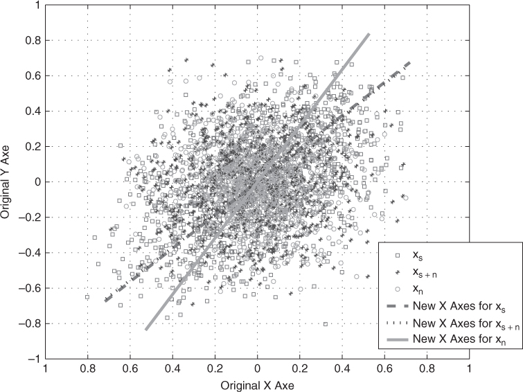
Assume we have 2 × 1 random vectors x_{s + n} = x_s + x_n, where x_s is vectorized sine sequence and x_n is the vectorized WGN sequence. SNR is set to 0 dB. There are 1000 samples for each random vector in Figure 2.1. Now we use eigen-decomposition to set the new X axes for each random vector samples such that λ₁ is strongest along the corresponding new X axes. It can be seen that new X axes for x_s (SNR = ∞ dB) and x_{s + n} (SNR = 0 dB) are almost the same. X axes for x_n (SNR = − ∞), however, is rotated with some random angle. This is because WGN has almost the same energy distributed in every direction. New X axes for noise will be random and unpredictable but the direction for the signal is very robust.

Based on leading eigenvector, feature template matching is explored for spectrum sensing. The secondary user receives the signal y(t). Based on the received signal, there are two hypotheses: one is that the primary user is present , another one is the primary user is absent . In practice, spectrum sensing involves detecting whether the primary user is present or not from discrete samples of y(t).

2.135

in which x(n) are samples of the primary user's signal and w(n) are samples of zero mean white Gaussian noise. In general, the algorithms of spectrum sensing aim at maximizing corresponding detection rate at a fixed false alarm rate with low computational complexity. The detection rate P_d and false alarm rate P_f are defined as

2.136

in which prob represents probability.

The hypothesis detection is

2.137

Assume the primary user's signal is perfectly known. Given d-dimensional vectors x₁, x₂, ···, x_M of the training set constructed from the primary user's signal, the sample covariance matrix can be obtained by

2.138

which assumes that the sample mean is zero,

2.139

The leading eigenvector of R_x can be extracted by eigen-decomposition of R_x,

2.140

where is a diagonal matrix. λ_i, i = 1, 2, ···, d are eigenvalues of R_x. V is an orthonormal matrix, the columns of which v₁, v₂, ···, v_d are the eigenvectors corresponding to the eigenvalues λ_i, i = 1, 2, ···, d. For simplicity, take v₁ as the eigenvector corresponding to the largest eigenvalue. The leading eigenvector v₁ is the template of PCA.

For the measurement vectors y_i, i = 1, 2, ···, M, the leading eigenvector of the sample covariance matrix is . Hence, the presence of signal is determined by [84, 85],

2.141

where T_pca is the threshold value for PCA method, and ρ is the similarity between and template v₁ which is measured by cross-correlation. T_pca is assigned to arrive a desired false alarm rate. The detection with leading eigenvector under the framework of PCA is simply called PCA detection.

A nonlinear version of PCA—kernel PCA [86]—has been proposed based on the classical PCA approach. Kernel function is employed by kernel PCA to implicitly map the data into a higher dimensional feature space, in which PCA is assumed to work better than in the original space. By introducing the kernel function, the mapping φ need not be explicitly known which can obtain better performance without increasing much computational complexity.

The training set x_i, i = 1, 2, ···, M and received set y_i, i = 1, 2, ···, M in kernel PCA are obtained the same way as with the PCA framework.

The training set in the feature space are φ(x₁), φ(x₂), …, φ(x_M) which are assumed to have zero mean, for example, . The sample covariance matrix of φ(x_i) is

2.142

Similarly, the sample covariance matrix of φ(y_i) is

2.143

The detection algorithm with leading eigenvector under the framework of kernel PCA is summarized here as follows [85]:

T_kpca is the threshold value for kernel PCA algorithm. The detection with leading eigenvector under the framework of kernel PCA is simply called kernel PCA detection.

DTV signal [87] captured in Washington D.C. will be employed to the experiment of spectrum sensing in this section. The first segment of DTV signal with L = 500 is taken as the samples of the primary user's signal x(n).

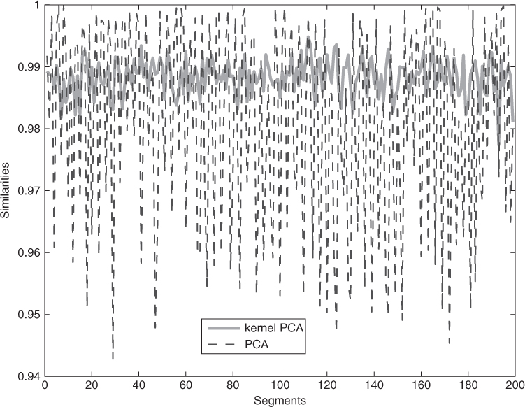
First, the similarities of leading eigenvectors of the sample covariance matrix between first segment and other segments of DTV signal will be tested under the frameworks of PCA and kernel PCA. The DTV signal with length 10⁵ is obtained and divided into 200 segments with the length of each segment 500. Similarities of leading eigenvectors derived by PCA and kernel PCA between the first segment and the rest 199 segments are shown in Figure 2.2. The result shows that the similarities are very high between leading eigenvectors of different segments' DTV signal (which are all above 0.94), on the other hand, kernel PCA is more stable than PCA.

The detection rates varied by SNR for kernel PCA and PCA compared with estimation-correlator (EC) and maximum minimum eigenvalue (MME) with P_f = 10% are shown in Figure 2.3 for 1000 experiments.

Experimental results show that kernel methods are 4 dB better than the corresponding linear methods. Kernel methods can compete with EC method.

2.6 Cyclostationary Detection

Generally, noise in the communication system can be treated as wide-sense stationary process. Wide-sense stationary has time invariant autocorrelation function. Mathematically speaking, if x(t) is a wide-sense stationary process, the autocorrelation function of x(t) is

2.147

and

2.148

Generally, manmade signals are not wide-sense stationary. Some of them are cyclostationary [88]. A cyclostationary process is a signal exhibiting statistical properties which vary cyclically with time [89]. Hence, if x(t) is a cyclostationary process, then

2.149

where T₀ is the period in t not in τ.

Define cyclic autocorrelation function for x(t) as

2.150

where α is cyclic frequency. If the fundamental cyclic frequency of x(t) is α₀, is nonzero only for integer multiples of α₀ and identically zero for all other values of α [88, 90, 91]. And spectral correlation function of x(t) can be given as

2.151

where PSD is a special case of spectral correlation function when α is zero.

In practice, can also be calculated based on the two following steps [92]:

Both cyclic autocorrelation function and spectral correlation function can be used as features to detect x(t) [88, 92]. Assume x(t) is the signal and w(t) is AWGN. The observed signal y(t) is equal to x(t) + w(t). The optimal cyclostationary detector based on spectral correlation function can be [92–94],

2.154

A novel approach to signal classification using spectral correlation and neural networks has been presented in [95]. α-profile is used as the feature in neural network for signal classification. The signal types under investigation include BPSK, QPSK, FSK, MSK, and AM [95]. α-profile is defined as [95],

2.155

where is the spectral coherence function of x(t) [95],

2.156

Similarly, signal classification based on spectral correlation analysis and SVM in cognitive radio has been presented in [96].

A low-complexity cyclostationary based spectrum sensing for UWB and WiMAX coexistence has been proposed in [97]. The cyclostationary property of WiMAX signals because of the cyclic prefix is used [97]. Cooperative cyclostationary spectrum sensing in cognitive radios has been discussed in [94, 98]. Cooperative spectrum sensing can improve the performance by the multiuser diversity [94]. The cyclostationary detector requires long detection time to obtain the feature, which causes inefficient spectrum utilization [99]. In order to address this issue, the sequential detection framework is applied together with the cyclostationary detector [99].

In an OFDM based cognitive radio system, cyclostationary signatures, which may be intentionally embedded in the communication signals, can be used to address a number of issues related to synchronization, blind channel identification, spectrum sharing and network coordination [100–102]. Hence, we can design cyclostationary signatures and the corresponding spectral correlation estimators for various situations and applications.

Besides, the blind source separation problem with the assumption that the source signals are cyclostationary has been studied in [103]. MMSE reconstruction for generalized undersampling of cyclostationary signals has been presented in [104]. Signal-selective direction of arrival (DOA) tracking for wideband cyclostationary sources has been discussed in [105]. Time difference of arrival (TDOA) and Doppler estimation for cyclostationary signals based on multicycle frequencies has been considered in [106].