
Chapter 6
Convex Optimization
Optimization refers to minimizing or maximizing the objective function by systematically choosing the values of optimization variables from or within an allowed set defined by the constraint functions. Many engineering problems can be effectively characterized in the form of optimization. Thus, optimization theory is a powerful tool to solve engineering problems. In order to map from engineering problem to optimization issue, objectives, constraints, and variables should be extracted from the engineering problem and expressed in a mathematical fashion. Objective can be the key performance metric we care about. In wireless communication, objective can be capacity or throughput. For the radar system, detection rate can be the design goal. For smart grid, the total cost for purchasing power should be minimized. Constraints are the physical limits of the system or the performance requirements. Variables can be the adjustable or controllable parameters in the system, for example, weights, gains, power, and so on. Besides, optimality, feasibility, and sensitivity should also be taken into account. Reasonable constraints should be set for the optimization problem, and active constraints should be given more attention.
There are many categories of optimization formats:
- Linear optimization and nonlinear optimization.
- Discrete optimization and continuous optimization.
- Deterministic optimization and stochastic programming.
- Constrained optimization and unconstrained optimization.
- Convex optimization and nonconvex optimization.
Convex optimization is a subfield of optimization theory, which studies the problem of minimizing convex objective function based on a compact convex set. The strength of convex optimization is if a local minimum exists, then it is a global minimum. Thus, if the engineering problem can be formulated as convex optimization, then global optimal solution can be obtained. That is one reason why convex optimization has recently become popular.
The other reason for the popularity of convex optimization is that convex optimization can be solved by cutting plane method, ellipsoid method, subgradient method, or interior point method. Thereinto, interior point method is widely used. This method consists of a self-concordant barrier function used to encode the convex set and reaches an optimal solution by traversing the interior of the feasible region. The interior point method can guarantee that the number of iterations is bounded by a polynomial in the dimension and accuracy of the solution.
Convex optimization can be used in any engineering field. The popular topic in sensing and image processing is compressive sensing (CS) which finds the sparse solution to the underdetermined linear equations using the prior knowledge that the solution is sparse or compressible. CS is formulated as minimizing the l1 norm which is convex optimization. Though the core of CS is optimization theory, CS can be still treated as a dedicated theory because of its particularity and significance. Though the sparse signal reconstruction has existed for at least four decades, this field has recently exploded, partially due to several important results by David Donoho, Emmanuel Candes, Justin Romberg, and Terence Tao. Besides, Lawrence Carin and his colleagues have built a new Bayesian framework for solving the inverse problem of CS [384, 385] and estimating a distribution for the unknown parameters. CS has been used for radar imaging in [386]. In cognitive radar network, though the data are huge, a sparse representation of data is still preferred. Thus, we should explore the method to learn the optimal dictionary for data representation [387]. Meanwhile, CS shows that physically sparse signal can be recovered from far fewer samples than the signal dimension [387]. Hence we should also find the optimal sensing matrix to project signals to the small amount of data with improving performance of reconstruction accuracy. In this way, the amount of data or information needed for radar signal processing can be greatly reduced. Furthermore, the overhead of cognitive radar network can be reduced.
It is also worth noting that the contribution of convex optimization to machine learning is significant. Learning the kernel matrix with SDP has been discussed in [388]. Learning multiresolution models with in-scale conditional covariance is formulated as convex optimization in [389]. E. J. Candes and his colleagues discuss robust PCA and try to decompose a data matrix into a low rank component and a sparse component by solving a convex program called principal component pursuit (PCP). Thus, it is safely foreseeable that convex optimization will play an important role in the function of cognition in the near future.
The standard format of convex optimization problem is [8],
where f0(x), f1(x), …, fM(x) are all convex functions, which means,
6.2 ![]()
for any θ with 0 ≤ θ ≤ 1 and all x1 as well as x2 which lies in a convex set [8].
In the convex optimization problem (6.1), x is the optimization variable. x can be a scaler, a vector or even a matrix. f0(x) is the objective function. fm(x), m = 1, 2, …, M are called constraint functions.
In mathematics, a concave function is the negative of a convex function. A function f(x) is concave over a convex set if and only if − f(x) is a convex function over the same set. If we would like to maximize one concave function, we can minimize its corresponding convex function.
The well-known convex functions or concave functions are listed as follows [8, 390]. The readers can refer to [8] for the definitions of notations.
- f(x) = eax is convex on R for any a ∈ R.
- f(x) = logx is concave on R++.
- f(x) = xa is convex on R++ if a ≥ 1 or a ≤ 0 and concave if 0 ≤ a ≤ 1.
- Every norm on RN is convex.
- f(x) = xlogx is convex on R++.
- f(x) = max{x1, x2, …, xN} is convex on RN.
 is convex on RN.
- The geometric mean
 is concave on
  .
.  is convex on R × R++.
- f(X) = logdet X is concave on
 .
. - f(X) = λmax(X) is convex on X ∈ SN where λmax(X) means maximum eigenvalue of a matrix.
- f(X) = trace (X−1) is convex on
 .
.  is concave on
  .
.- If A is positive definite matrix A ∈ CN×N, f(X) = trace (XAXH) is strictly convex.
6.1 Linear Programming
If the objective and constraint functions are all linear, the optimization problem is called a linear programming. Linear programming is one kind of convex optimization problems. A general linear programming has the form [8],
6.3 
where x ∈ RN, a ∈ RN, C ∈ RM×N, d ∈ RM, G ∈ RL×N, and h ∈ RL.
A standard form linear programming is expressed as [8],
6.4 
where the only inequality constraints are component-wise nonnegativity constraints ![]() . An inequality form linear programming is written as [8],
. An inequality form linear programming is written as [8],
6.5 
where no equality constraints exist.
6.2 Quadratic Programming
If the linear objective function in linear programming are replaced by the convex quadratic objective function, the corresponding optimization problem is called quadratic programming which can be expressed as [8],

where ![]() and q ∈ RN.
and q ∈ RN.
Furthermore, if the inequality constraints ![]()
in the quadratic programming (6.6) is replaced by the convex quadratic constraints, the corresponding optimization problem is called quadratically constrained quadratic programming (QCQP) which can be expressed as [8],
6.7 
where ![]() and qm ∈ RN, m = 0, 1, 2, …, M.
and qm ∈ RN, m = 0, 1, 2, …, M.
The norm cone related to the norm || · || is the convex set which can be expressed as [8],
6.8 ![]()
If l2 norm is considered, the corresponding cone is called second-order cone, quadratic cone, or ice-cream cone.
If the convex quadratic constraints in QCQP are replaced by the convex second-cone constraints, the corresponding optimization problem is called SOCP [8],
6.9 
where ![]() and
and ![]() .
.
6.3 Semidefinite Programming
If ![]() , X is a positive-semidefinite matrix or nonnegative-definite matrix which means
, X is a positive-semidefinite matrix or nonnegative-definite matrix which means
6.10 ![]()
for all u ∈ RN. If X is a positive-semidefinite matrix, then all eigenvalues of X are nonnegative and all diagonal entries in X are nonnegative.
SDP is a subfield of convex optimization. SDP tries to optimize a linear objective function over the intersection of the cone of positive semidefinite matrices with an affine space. SDP based signal processing is becoming more and more popular recently. It can be applied to control theory, machine learning, statistics, circuit design, graph theory, quantum mechnics [164], and so on. The reasons for this are
- More and more practical problems can be formulated as SDP.
- Many combinatorial and nonconvex optimization problems can be relaxed to SDP.
- Most of the interior-point methods for linear programming have been generalized to SDP [391].
- The computational capability is increased greatly and SDP can be solved efficiently.
Hence, SDP serves as a core convex optimization format.
SDP has the form [8],
6.11 
where F1, F2, …FN, E ∈ SK.
Similar to linear programming, a standard form SDP is expressed as [8],
6.12 
where A, F1, F2, …, FM ∈ SN and a matrix nonnegativity constraint is imposed on the variable X ∈ SN.
6.4 Geometric Programming
Geometric programming is a class of optimization problems. The standard form of geometric programming itself is nonlinear and nonconvex. However, geometric programming can be easily transformed to convex optimization problem [8, 392]. In this way, a global optimum can be obtained.
If a function is defined as,
6.13 ![]()
where c, x1, x2, …, xN ∈ R++ and a1, a2, …, aN ∈ R, this function is called a monomial function, or simply, a monomial [8].
A sum of monomials is a posynomial function, or simply, a posynomial [8],
6.14 
where ck ∈ R++ and a1k, a2k, …, aNk ∈ R, k = 1, 2, …, K.
A standard form of geometric programming has the form [8],

where f0, f1, f2, …, fM are posynomials and h1, h2, …, hL are monomials.
Define,
6.16 ![]()
then,
6.17 ![]()
A monomial can be transformed to [8]
6.18 
where b = logc. The change of variables turns a monomial function into the exponential of an affine function [8].
Similarly, a posynomial can be transformed to [8]
6.19 
where ak = (a1k, a2k, …, aNk)T and bk = logck, k = 1, 2, …, K.
The geometric programming (6.15) can be expressed in terms of y ∈ RN as [8],

where amk ∈ RN, m = 0, 1, 2, …, M and gl ∈ RN, l = 1, 2, …, L.
Finally, we perform logarithm operation to the objective function and constraint functions in the geometric programming (6.20) to get the convex form of geometric programming [8],
If the objective function and constraint functions in the geometric programming (6.21) are all monomials, then the geometric programming (6.21) reduces to a linear programming. Hence, geometric programming can be treated as an extension of linear programming [8].
Extensions of geometric programming are documented in [392] together with applications in communication systems. These applications include channel capacity, coding, network resource allocation, network congestion control, and so on [392].
6.5 Lagrange Duality
In optimization theory, the duality theory states that optimization problems may be viewed from either of two perspectives, the primal problem or the dual problem. No matter whether the primal problem is convex or not, the dual problem is certainly concave. Thus, the dual problem is easy to solve. The solution of the dual problem provides a lower bound to the solution of the primal problem.
Mathematically speaking, if the primal problem, which is not necessarily convex, is expressed as
and its optimal value is
6.23 ![]()
then the corresponding dual problem is
6.24 
where g(λ, υ) is Lagrange dual function defined as [8]
6.25 
and x satisfies constraints in the primal problem (6.22).
Denote the optimal value of the dual problem by d*. Weak duality always holds for convex and nonconvex problems,
6.26 ![]()
and strong duality usually holds for convex problems,
6.27 ![]()
6.6 Optimization Algorithm
Two categories of algorithms, that is, deterministic algorithms and stochastic algorithms, are widely used to solve optimization problems. For deterministic algorithms, interior point methods are very popular recently.
6.6.1 Interior Point Methods
Interior point methods are a class of algorithms to solve linear and nonlinear convex optimization problems. Ideally, any convex optimization problems can be solved by interior point methods. The key element of these methods is to use a self-concordant barrier function to encode the convex set [393]. A barrier function is a continuous function whose value on a point increases to infinity as the point approaches the boundary of the feasible region. Thus, interior point methods reach an optimal solution by going through the interior of the feasible region.
The ideal barrier function should be [8],
6.28 ![]()
In reality, logarithmic barrier is used as an approximation,
6.29 ![]()
where t > 0 and approximation improves as t goes to infinity [8]. Meanwhile, logarithmic barrier function is convex and twice continuously differentiable.
6.6.2 Stochastic Methods
Stochastic methods or random search methods generate and use random variables to get the solution to the optimization problem. Stochastic methods do not need to explore the structures of objective functions and constraints, that is, derivative or gradient information. Stochastic methods will be suitable for the nonconvex optimization problems or the relatively large-scale high-dimension optimization problems. Stochastic methods cannot guarantee the global optimum, but there are often no other choices.
Stochastic methods can include but are not limited to
- simulated annealing;
- stochastic hill climbing;
- genetic algorithm;
- ant colony optimization;
- particle swarm optimization (PSO).
Therein, genetic algorithm, which is one kind of evolutionary algorithm techniques, has been widely used for multiobjective optimization or multiobjective decision making. Take PSO as an example [394]. Power allocation problem for time reversal with array gain in MIMO UWB system is formulated as a nonconvex optimization issue. Even though the first and second derivatives of the objective functions and constraints can be easily derived [394], because the objective function is a nonlinear and nonconvex function, it is hard to use deterministic algorithm to solve this optimization problem. PSO is applied [394]. PSO is a swarm intelligence based algorithm to find a solution to an optimization problem [395]. There are many particles with a position and a velocity in the swarm. Particles in a swarm communicate good positions to each other and adjust their own position and velocity based on these good positions.
Suppose there are N particles. After K iterations, the algorithm is stopped. When the k-th iteration begins, the position of particle i is ![]() . The velocity of particle i is
. The velocity of particle i is ![]() . The local best position of particle i is
. The local best position of particle i is
6.30 ![]()
where C(L) is the utility function. The global best position is
6.31 ![]()
Then the velocity of particle i in the k-th iteration is
and the new position of particle i is ![]() . In Equation (6.32) rand means random value drawn from a uniform distribution on the unit interval; w is the inertia weight; c1 and c2 are two positive constants, called the cognitive and social parameter respectively.
. In Equation (6.32) rand means random value drawn from a uniform distribution on the unit interval; w is the inertia weight; c1 and c2 are two positive constants, called the cognitive and social parameter respectively.
6.7 Robust Optimization
The optimization issue with uncertainty is becoming hotter and hotter in many research fields, such as operation research, finance, industrial management, transportation scheduling, wireless communication, smart grid, and so on, because most of the optimization issues are from the dynamic complex system, and most of the variables in the optimization issue cannot be deterministic or known for sure. There are two approaches to deal with the optimization issue with uncertainty. One is robust optimization, and the other is stochastic optimization. In robust optimization, the uncertainty model is deterministic and set based [396]. However, in stochastic optimization, the uncertainty model is assumed to be random [396]. Robust optimization, which is a conservative approach [397], can guarantee the performance for all the cases within the set based uncertainty. In other words, robustness means the performance is stable with the bounded errors. However, stochastic optimization can only guarantee the performance on average for the uncertainty with known or partially known probability distribution [397] information. Thus, there is a tradeoff between robustness and performance. Robust optimization will materialize by waveform diversity.
Waveform diversity is a key research issue in the current wireless communication system, the radar system, and the sensing or image system. Waveform should be designed or optimized according to the different requirements or objectives of system performance and should be adapted or diversified dynamically to the operating environment in order to achieve a performance gain [398]. For example, the waveform should be designed to carry more information to the receiver in terms of capacity. If the energy detector is employed at the receiver, the waveform should be optimized such that the energy of the signal in the integration window at the receiver should be maximized [399–401]. For navigation and geolocation, the ultra short waveform should be used to increase the resolution. For multi-target identification, the waveform should be designed so that the returns of radar signals can bring more information back. In clutter dominant environment, maximizing the target energy and minimizing the clutter energy should be considered simultaneously.
Multiple input single output (MISO) system is one kind of multi-antenna systems in which there are multiple antennas at the transmitter and one antenna at the receiver. MISO system can explore the spatial diversity and execute the transmitter beamforming to focus energy on the desired direction or point and avoid interference to other radio systems. It is well known that waveform and spatially diverse capabilities are made possible today due to the advent of lightweight digital programming waveform generator [402] or AWG. Waveform diversity can also be applied to the wideband system. Waveform design or optimization for wideband multi-antenna system is documented in [403]. From a theoretical point of view, the contribution of [403] can be summarized as follows. The equivalent baseband waveforms are designed for the passband system. Different waveforms for different transmitter antennas are jointly optimized to obtain the global optimality. At the receiver, the received signals from different transmitter antennas will be combined together over the air such that the receiver antenna will see only one copy of the signal from the transmitter. In order to achieve this kind of over the air coherency for the passband signals, all the individual oscillators should be tied together at the transmitter [402] to make the carrier phase consistent.
In the context of cognitive radio, waveform design gives us flexibility to design radio, which can coexist with other cognitive radios and primary radios. From cognitive radio's point of view, spectral mask constraint at the transmitter and the interference cancellation at the receiver should be seriously considered for waveform design or optimization, in addition to the traditional communication objectives and constraints. Spectral mask constraint is imposed on the transmitted waveform such that cognitive radio has limited or no interference to primary radio. At the same time, the interference cancellation scheme is implemented at the receiver to cancel the interference from primary radio to cognitive radio.
Though the thought of waveform diversity for the radar system can be traced back to World War II, due to the computational capability and hardware limitation, a lot of waveform design algorithms cannot be implemented into the radar system [398] for many years. Nowadays, these bottlenecks are broken, and waveform diversity becomes a hotspot afresh in the radar society. Time reversal or phase conjugating waveform, colored waveform, sparse and regular nonuniform Doppler waveform, noncircular waveform, and so on are dealt with based on advanced mathematics tools in [404]. New trends in coded waveform design for radar applications are presented in [405]. The modern SDP and the novel algorithm on Hermitian matrix rank one decomposition are exploited to perform code selection which can maximize the detection performance and control the Doppler estimation accuracy and the similarity with a prefixed radar code [405]. Meanwhile, another force to propel the research on waveform diversity is the introduction of cognition to the radar system, that is, cognitive radar which means the radar can actively learn about the environment, and the whole radar system forms a dynamic closed feedback loop including the transmitter, environment, and receiver [406]. Waveform diversity will play an important role in cognitive radar. The radar transmitter can adjust its illumination of the environment in an intelligent, effective, adaptive, and robust manner, taking into account the results of learning and perception [406]. Thus, the philosophy of sequential testing [407] can be embraced under the umbrella of cognitive radar smoothly. Several rounds of illuminations will be used until the belief that the decision is correct is made. The waveform and the transceiver scheme for each round can be adjustable according to the results of the previous illuminations. For example, adaptive CS [384] gives us the hint to this research field. Though the thought of waveform diversity for the radar system can be traced back to World War II, due to the computational capability and hardware limitation, a lot of waveform design algorithms cannot be implemented into the radar system [398] for many years. Nowadays, these bottlenecks are broken, and waveform diversity becomes a hotspot afresh in the radar society. Time reversal or phase conjugating waveform, colored waveform, sparse and regular nonuniform Doppler waveform, noncircular waveform, and so on are dealt with based on advanced mathematics tools in [404]. New trends in coded waveform design for radar applications are presented in [405]. The modern SDP and the novel algorithm on Hermitian matrix rank one decomposition are exploited to perform code selection which can maximize the detection performance and control the Doppler estimation accuracy and the similarity with a prefixed radar code [405]. Meanwhile, another force to propel the research on waveform diversity is the introduction of cognition to the radar system, that is, cognitive radar which means the radar can actively learn about the environment, and the whole radar system forms a dynamic closed feedback loop including the transmitter, environment, and receiver [406]. Waveform diversity will play an important role in cognitive radar. The radar transmitter can adjust its illumination of the environment in an intelligent, effective, adaptive, and robust manner, taking into account the results of learning and perception [406]. Thus, the philosophy of sequential testing [407] can be embraced under the umbrella of cognitive radar smoothly. Several rounds of illuminations will be used until the belief that the decision is correct is made. The waveform and the transceiver scheme for each round can be adjustable according to the results of the previous illuminations. For example, adaptive CS [384] gives us the hint to this research field.
The previous theoretical researches on waveform diversity do not take the robustness into account. There are several reasons for this:
- The theory of robust optimization was not that mature in the old days.
- Robustness makes waveform diversity complex.
- The research on waveform diversity was only limited to computer simulation.
Nowadays, as the theory of robust optimization becomes mature and bottlenecks of computation and implementation are broken, robust optimization for waveform diversity, that is, robust waveform diversity, will bring more attention. Meanwhile, robustness is the bridge between the theoretical work and the practical situation.
Robust optimization is the key mathematical tool for robust waveform diversity, which gives the optimal waveform with robustness. Robust optimization is systematically introduced in [396]. The most frequently used optimization formats within robust optimization are robust linear programming [396, 408, 409], robust least squares [8, 410], robust mean square error (MSE) [411–417], and robust SDP [418, 409]. If the optimization issues can be formulated as robust linear programming, robust least squares, or robust MSE with some specific uncertainty models, these optimization issues will be solvable and tractable. For example, if the uncertainty model is the ellipsoidal uncertainty set, robust linear programming becomes an SOCP and a robust SOCP becomes an SDP [419], which can be efficiently solved via interior point methods. However, a robust SDP with the ellipsoidal uncertainty set is NP-hard to solve [419]. Because SDP is harder than SOCP, and SOCP is harder than linear programming taking the complexity of solving method into account, robustness increases the difficulty of the optimization issue [419]. Robust least squares with the finite uncertainty set, norm bound error, uncertainty ellipsoids, and norm bounded error with linear structure are discussed in [8]. Meanwhile, the solution of robust least squares where the coefficient matrices are unknown but bounded is also given in [410]. The worst case residual is minimized, and the corresponding optimization problem can be formulated as SOCP. The work on robust MSE is done by [411–417] from classical estimation's point of view. Robust MSE can also be called minimax MSE. The core idea of the competitive minimax approach [412] is to seek the linear estimator that minimizes the worst case regret with the assumption that the covariance of parameter vector is subject to uncertainties. The minimax MSE estimator, the linear estimator that minimizes the worst case MSE among all parameter vectors with bounded norm [414], can be found by solving an SDP. Similarly, robust MSE with noise covariance uncertainty is dealt with in [415]. Robust MSE is extended to a multisignal estimation issue in [416] where both model and noise uncertainties are considered.
Transmitter power control can be treated as one kind of waveform diversity schemes. Traditionally, power control or power allocation was implemented above the physical layer as one kind of radio resource management issues. Power control can be implemented in the physical layer. In this way, the period of power control loop will be greatly reduced. Different power control patterns will synthesize different transmitted waveforms to meet different requirements. Robust transmitter power control is documented in [397]. OFDM modulation scheme is adopted in the physical layer. Every cognitive radio should dynamically control the transmission powers for its own subcarriers in order to maximize the total benefits. Thus, the objective of this optimization issue is the maximization of total capacities of all cognitive radios, and the constraints consist of the individual power constraints and interference constraints. Because there is no central node in cognitive radio network, the feasible algorithm to solve this optimization issue should be implemented in a decentralized manner. For the nonrobust version of optimization issue, the classical iterative waterfilling can be used, and the convergence of the solution can be guaranteed. However, the cognitive radio network has a dynamic nature [397] due to the random mobility of cognitive radios and primary radios. Thus the noise plus interference term includes two components: a nominal term and a perturbation term to form the robust version of optimization issue. The price of the robustness is that a convex optimization problem becomes a nonconvex optimization problem. Most of the algorithms for convex optimization cannot be used. A new numerical technique to solve the nonconvex robust optimization issue is proposed in [420]. Neighborhood searches and robust local moves are applied iteratively to achieve the robust solutions [397]. Similar to transmitter power control, transmitter beamforming can be thought of as another kind of waveform diversity schemes. Robust transmitter beamforming in multiuser MISO cognitive radio networks is considered in [421]. Channel state information in [421] is assumed to be imperfectly known, and the imperfectness of channel state information is modeled using an Euclidean ball shaped uncertainty set [421]. Specifically speaking, the objective is to design the optimal beamforming weights for different cognitive radios with the least total transmitted power at the central node while simultaneously the least possible received signal to interference plus noise ratio (SINR) for each cognitive radio should be equal to or greater than a threshold defined by the quality of service (QoS) requirement. The interference for each primary radio should be equal to or less than a threshold to make primary radio work properly. Robust transmitter beamforming with partial channel state information for cognitive radio can also be seen in [422]. Because of the limitation of sounding system and feedback system, robustness to partial channel state information, channel state information error, or the limited feedback is very important to dealing with transmitter power control and beamforming. Meanwhile, due to the perturbation of the radio environment and the fading of the radio channel, how to deal with outdated channel state information is still worth studying. Sometimes, without channel state information, the directional beam for far field can still be formed at the transmitter using array manifold, steering vector, or spatial signature.
Robust waveform diversity is applied to MIMO radar system in [423]. The design criteria are mutual information and MMSE estimation for target identification and classification. Target PSD is assumed to lie in an uncertainty class of spectra bounded by known upper and lower bounds [423]. With this kind of prior information, the designed waveform can well match the target and bring back more information. The minimax robust waveforms can bound the worst case performance at an acceptable level [423]. Optimal and robust waveform design for MIMO radars with the consideration of the signal dependent noise, that is, clutter, is studied in [424]. Robust waveforms to minimize the estimation error of the worst case target realization are obtained [424].
It has been widely accepted that waveform diversity is implemented at the transmitter. But waveform diversity should have broader meaning and significance. First of all, any type of signal processing in the waveform level at the receiver should also be included into the waveform diversity framework. The most common signal processing is the receiver beamforming including the narrowband beamforming and wideband beamforming. Robust receiver beamforming is dealt with in [425, 426]. The uncertainty comes from the mismatch of steering vector and the estimation error of the sampled covariance matrix for interference plus noise. The worse case performance of the minimum variance beamformer or Capon beamformer is taken care of. SDP or SOCP can be exploited to solve the corresponding robust optimization issues. Robust minimum variance beamformer with probabilistic constraint is mentioned in [427], and the relationship between probability constrained and worst case optimization is discussed. Robust least squares are applied to antenna design in [409]. The optimal solution obtained from the nominal least squares is completely unstable w.r.t. small implementation errors [409]. However, robust least squares will bring stable results to combat the uncertainty. Robust wideband beamforming is addressed and presented by [428]. Similarly, error from steering vector brings instability to the system and inevitably degrades the beamformer's performance [428]. Hybrid steepest descent method is proposed to find the unique minimizer of the cost function over the feasible convex set [428].
6.8 Multiobjective Optimization
Practical optimization problems, especially the engineering design optimization problems, seem to have a multi-objective nature much more frequently than a single objective one [429]. For example, to form wideband beampattern with arbitrary shape, we need to consider at least four objectives: main beam, sidelobe, nulling, and frequency invariant property.
In terms of solution, the difference between the multiobjective optimization and the single-objective optimization is the former has a set of Pareto-optimal solutions while the latter has a single global optimum if such a solution exists. The term “Pareto-optimal solution” refers to a solution around which there is no way of improving any objective without worsening at least one other objective [429]. The set of Pareto-optimal solutions can be characterized by Pareto front—a hypersurface in the objective function space in which the Pareto-optimal points are located [429].
How to get the solution for the multiobjective optimization is based on how the individual objective should be weighted in relation to all others. Thus, four kinds of methods can be applied in terms of preference [429, 430]:
- A Priori Preference. We can specify the preferences before running the optimization algorithm. Most likely, a single utility function is developed to combine all the objectives.
- Progressive Preference. We can interact with the optimization algorithm and change the preferences during the optimization process.
- A Posteriori Preference. No preferences is given before or during the optimization process. We can choose the solution from a set of candidates provided by the optimization algorithm.
- No Preference. No preferences are needed in the whole process of the multiobjective optimization.
If preferences are given beforehand, the weighted sum method is the simplest approach and probably the most widely used classical method. This method transforms the multiobjective optimization problem into a single objective one by multiplying each objective with a predetermined weight and adding all the weighted objectives together. The solution to the single objective problem is Pareto-optimal if the weights are positive for all objectives. However, the weighted sum method cannot guarantee that any Pareto-optimal solution can be obtained using a positive weight vector. Meanwhile, if preferences are not given beforehand, we have to find a set of candidate solutions as completely as possible.
For deterministic strategy, ε-constraint method, weighted metric methods, rotated weighted metric method, value function method, and so on can be exploited. Besides, stochastic algorithms, especially evolutionary algorithms, seem to be more popular than deterministic algorithms to solve the multiobjective optimization problem [430–433]. Convergence and diversity are two important issues for multiobjective evolutionary algorithms [434]. An efficient evolutionary method to approximate the Pareto optimal set in multiobjective optimization has been proposed in [435]. A relevant example is to use strength Pareto evolutionary algorithm 2 to design simultaneous multimission waveforms [436]. A genetic algorithm is also applied in [437] to obtain OFDM radar waveform for target detection with consideration of error bound and Mahalanobis-Distance. Similarly, in order to make algorithms scalable, parallel genetic algorithms [438] are worth using.
The performance optimization of cognitive radio or cognitive radio network itself is a multi-objective optimization problem. First of all, multiple objectives exist from physical layer to application layer in cognitive radio network [439]. Different layers may have different performance metrics. Different applications may have different QoS requirements. Different users may have different subjective performance needs. Hence, multiple objectives should be taken into account simultaneously. Meanwhile, the external radio environment and internal network state determine the validity, feasibility, and sensitivity of objectives. Specifically speaking, bit error rate (BER) minimization, out-of-band interference minimization, power consumption minimization, and overall throughput maximization have been achieved using a multiobjective fitness function in the framework of distributed optimization [440, 441]. Genetic algorithm and its variants are widely exploited [441–449]. Besides, PSO can also be used for spectrum allocation in cognitive radio network with consideration of sum bandwidth reward and access fairness of secondary users [450]. From the perspective of artificial intelligence, a case-based reasoning method using the divide-and-conquer concept has been explored to generate solutions for problems with multiple objectives in cognitive radio [451].
6.9 Optimization for Radio Resource Management
Radio resource management is the system-level control for the wireless communication system [452–457]. Generally, radio resource management tries to optimize the utilization of various radio resources such that the performance of radio system can be improved. Mathematical optimization, especially convex optimization, is the main tool supporting radio resource management [458]. Meanwhile, radio resource management will be the basic function in cognitive radio [459]. Spectrum related management for spectrum sensing spectrum access, spectrum sharing, and so on, will be the feature for cognitive radio [460, 461].
Radio resource management includes but is not limited to
- power control [462–467];
- frequency band allocation;
- time slot allocation;
- adaptive modulation and coding [468–470];
- rate control [471];
- antenna selection [472–475];
- scheduling [471, 476–479];
- handover [480–482];
- admission control [483–489];
- congestion control [484, 490–494];
- load control [495];
- routing plan [496–498];
- base station deployment.
The work about radio resource management can also be found in [499–507]. Capacity, communication rate, spectrum efficiency, or capacity region is used frequently as performance metric for radio resource management. Besides, MIMO related radio resource management and OFDM related radio resource management will also be mentioned in the following chapters.
6.10 Examples and Applications
The examples and applications will show the beauty and benefit of mathematical optimization.
6.10.1 Spectral Efficiency for Multiple Input Multiple Output Ultra-Wideband Communication System
It is assumed that there are Nt transmitter antennas and Nr receiver antennas in the system.
The channel transfer function is H(f) with bandwidth W = f1 − f0 where f0(> 0) is the starting frequency and f1(> 0) is the end frequency
6.33 
where Hmn(f) is channel transfer function from the transmitter antenna n to the receiver antenna m. Its corresponding channel impulse response is
6.34 
The spectrum shaping filter at the transmitter side is
6.35 
and its corresponding transfer function is
6.36 
The input of the spectrum shaping filter is the transmitted signal vector a(t). The entries of a(t) are a1(t), a2(t), …, and ![]() ,
,
6.37 
all of which are independent white Gaussian random processes with zero mean and unit PSD.
The transmitted signal at the transmitter array is
6.38 ![]()
where “⊗” denotes convolution operation and each entry of S(t) is
6.39 
Hence, the PSD of the transmitted signal at the transmitter array is
The received signal at the receiver array is
6.41 ![]()
where N(t) is AWGN the entries of which are independent random processes with zero mean and one-sided PSD N0.
If a one-sided situation is considered, then the transmitted power is
6.42 ![]()
The equivalent ratio of the transmitted signal power to the received noise power (TX SNR) is defined as
6.43 ![]()
The spectral efficiency is [508]
where | • | represents the determinant of the matrix.
The methods for the design of spectrum shaping filter are
- water filling;
- constant power water filling;
- time reversal;
- channel inverse;
- constant power spectral density;
- MMSE.
6.10.1.1 Water Filling
It is well known that the spectral efficiency of water filling is greater than that of any other spectrum shaping scheme. Let ![]() denote the set of eigenvalues of N0H−1(f)[H−1(f)]H. So SVD of N0H−1(f)[H−1(f)]H can be written as
denote the set of eigenvalues of N0H−1(f)[H−1(f)]H. So SVD of N0H−1(f)[H−1(f)]H can be written as
6.45 ![]()
where diag(a), if a is a vector with n components, returns an n-by-n diagonal matrix having a as its main diagonal. Because of the property of unitary matrix, ![]() can be expressed as
can be expressed as
6.46 ![]()
Then, RS(f) can be given by
6.47 ![]()
where ![]() and (x)+ = max[0, x]. Here, the constant μ is the water level chosen to satisfy the power constraint with equality
and (x)+ = max[0, x]. Here, the constant μ is the water level chosen to satisfy the power constraint with equality
6.48 
So, the spectral efficiency ![]() in this case is [509]
in this case is [509]
6.49 
6.10.1.2 Constant Power Water Filling
Constant power water filling is well studied in [510]. For water filling, the power allocation scheme is ![]() . While for constant power water filling, the power allocation scheme is
. While for constant power water filling, the power allocation scheme is
6.50 ![]()
How to get the optimal p0 and λ0 is the key point of constant power water filling. Similarly, the frequency band sets ![]() are defined as
are defined as
6.51 ![]()
The measure of Ωi is θi, and
6.52 
λ0 should be selected to meet the condition that ![]() is equal to
is equal to
6.53 ![]()
Meanwhile, ![]() .
.
6.10.1.3 Time Reversal
For time reversal, it follows that
6.54 ![]()
where the constant α is the scale factor chosen to satisfy the power constraint with equality,
6.55 
Hence
6.56 
and
6.57 
The spectral efficiency ![]() in this case is [509]
in this case is [509]
6.58 
6.10.1.4 Channel Inverse
For channel inverse, it follows that
6.59 ![]()
where the constant α is the scale factor chosen to satisfy the power constraint with equality,
6.60 
Hence
6.61 
and
6.62 
The spectral efficiency ![]() in this case is [509]
in this case is [509]
6.63 
6.10.1.5 Constant Power Spectral Density
If power is equally allocated to each transmitter antenna, then
6.64 ![]()
The spectral efficiency ![]() in this case is [509]
in this case is [509]
6.65 
6.10.1.6 Minimum Mean Square Error
For MMSE, it follows that
6.66 ![]()
where the constant α is the scale factor chosen to satisfy the power constraint with equality,
6.67 
So α is equal to
6.68 
Similarly, the spectral efficiency in this case can be calculated by Equation (6.40) and Equation (6.44).
6.10.2 Wideband Waveform Design for Single Input Single Output Communication System with Noncoherent Receiver
OOK modulation is considered and the transmitted signal is
6.69 
where Tb is the bit duration; p(t) is the transmitted bit waveform defined over [0, Tp]; and dj ∈ {0, 1} is j-th transmitted bit. Without loss of generality, assume the minimal propagation delay is equal to zero. The energy of p(t) is
6.70 ![]()
The received noisy signal at the output of the receiver front-end is
6.71 
where h(t), t ∈ [0, Th] is the multipath impulse response that takes into account the effects of channel impulse response and the RF front-ends of the transceivers including antennas. h(t) is available at the transmitter [511, 512]. n(t) is a low-pass additive zero mean Gaussian noise with one-sided bandwidth W and one-sided PSD N0. x(t) is the received noiseless bit-“1” waveform defined as
We further assume that Tb ≥ Th + Tp = Tx, that is, no existence of intersymbol interference (ISI).
An energy detector performs nonlinear square operation to r(t) without any explicit analog filter at the receiver. Then the integrator does the integration over a given integration window TI. Corresponding to the time index k, the k-th decision statistic at the output of the integrator is given by
6.73 
where TI0 is the starting time of integration for each bit, and 0 ≤ TI0 < TI0 + TI ≤ Tx ≤ Tb.
An approximately equivalent SNR for the energy detector receiver, which provides the same detection performance when applied to a coherent receiver, is given as [400]
For the best performance, the equivalent SNR SNReq should be maximized. Define
For given TI, N0, and W, SNReq is an increasing function of EI. So the maximization of SNReq in Equation (6.74) is equivalent to the maximization of EI in Equation (6.75).
The optimization problem to get the optimal waveform is shown as
In order to solve the optimization problem (6.76), numerical approach is employed. In other words, p(t), h(t), and x(t) are uniformly sampled, and the optimization problem (6.76) will be converted to its corresponding discrete time form. Assume the sampling period is Ts. Tp/Ts = Np. Th/Ts = Nh. Tx/Ts = Nx. So Nx = Np + Nh.
p(t), h(t), and x(t) are represented by pi, i = 0, 1, …, Np, hi, i = 0, 1, …, Nh, and xi, i = 0, 1, …, Nx, respectively [400].
Define
6.77 ![]()
and
6.78 ![]()
Construct channel matrix ![]()
6.79 ![]()
where (•)i, j denotes the entry in the i-th row and j-th column of the matrix or vector. Meanwhile, for vector, taking p as an example, (p)i, 1 is equivalent to pi−1.
The matrix expression of Equation (6.72) is
and the constraint in the optimization problem (6.76) can be expressed as
6.81 ![]()
where “|| • ||2” denotes the Euclidean norm of the vector. In order to make the whole document consistent, we further assume
6.82 ![]()
Let TI/Ts = NI and TI0/Ts = NI0. The entries in x within integration window constitute xI as,
6.83 ![]()
and EI in Equation (6.75) can be equivalently shown as
6.84 ![]()
Simply dropping Ts in EI will not affect the optimization objective, so EI is redefined as
Similar to Equation (6.80), xI can be obtained by
where ![]() , and i = 1, 2, …, NI + 1 as well as j = 1, 2, …, Np + 1.
, and i = 1, 2, …, NI + 1 as well as j = 1, 2, …, Np + 1.
The optimization problem (6.76) can be represented by its discrete time form as,

The optimal solution p* for the optimization problem (6.87) is the dominant eigenvector in the following eigendecomposition [400]
6.88 ![]()
Furthermore, ![]() will be obtained by Equation (6.85) and Equation (6.86).
will be obtained by Equation (6.85) and Equation (6.86).
6.10.2.1 Tradeoff between Energies Within and Outside Integration Window
In order to reduce ISI, the energies within and outside of integration window should be considered simultaneously, which means there is a tradeoff between energies within and outside integration window [401].
The entries in x outside of integration window constitute ![]() as
as
6.89 ![]()
and the energy outside of integration window ![]() can be expressed as
can be expressed as
6.90 ![]()
Similar to Equation (6.86), ![]() can be obtained by
can be obtained by
6.91 ![]()
where (![]() )i, j = (H)i, j when i = 1, …, NI0 and
)i, j = (H)i, j when i = 1, …, NI0 and ![]() when i = NI0 + NI + 2, …, Nx + 1 as well as j = 1, 2, …, Np + 1.
when i = NI0 + NI + 2, …, Nx + 1 as well as j = 1, 2, …, Np + 1.
In order to balance energies within and outside of integration window, the tradeoff factor α is introduced. The range of α is from 0 to 1. How to choose α depends on the performance requirement. Given α, the optimization problems is formulated as

The optimal solution p* for the optimization problem (6.92) is the dominant eigenvector in the following eigendecomposition [401]
6.93 ![]()
6.10.2.2 Binary Waveform
If the transmitted waveform is constrained to the binary waveform because of the hardware limitation or implementation simplicity, which means pi, i = 0, 1, …, Np is equal to ![]() or
or ![]() , then the optimization problem is
, then the optimization problem is

One suboptimal solution ![]() to the optimization problem (6.94) is derived from the optimal solution p* of the optimization problem (6.87). When p* is obtained, then
to the optimization problem (6.94) is derived from the optimal solution p* of the optimization problem (6.87). When p* is obtained, then
This simple method can lead to the optimal solution to the optimization problem (6.94) when TI → 0, which can be proved by Cauchy Schwarz inequality, but if TI is greater than zero, there is still an improvement potential to this suboptimal solution obtained from Equation (6.95).
Define
P should be a symmetric positive semidefinite matrix, that is, ![]() , and rank of P should be equal to 1. Reformulate EI as
, and rank of P should be equal to 1. Reformulate EI as
6.97 
Rank constraint is nonconvex constraint, so after dropping it, the optimization problem (6.94) is relaxed to
The optimal solution P* of the optimization problem (6.98) can be obtained by using CVX tool [513], and the value of the objective function in the optimization problem (6.98) gives the upper bound of the optimal value in the optimization problem (6.94). Projecting the dominant eigenvector of P* on ![]() and
and ![]() based on Equation (6.95), the suboptimal solution
based on Equation (6.95), the suboptimal solution ![]() is achieved [514].
is achieved [514].
Finally, the designed binary waveform is [401]
6.99 ![]()
6.10.2.3 Ternary Waveform
If the transmitted waveform is constrained to the ternary waveform, which means pi, i = 0, 1, …, Np is equal to three levels, that is, − c, 0 or c, then the optimization problem is expressed as
The optimization problem (6.100) is still NP-hard and can be approximately reformulated as

where Cardinality(p) denotes the number of nonzero entries of p, and cardinality constraint is also a nonconvex constraint.
Because k is the integer number between 1 and Np + 1, the optimization problem (6.101) can be decomposed into Np + 1 independent, and parallel subproblems and each subproblem is shown as
where k is equal to 1, 2, ···, or Np + 1.
Problem (6.102) can be solved in parallel, and then the solutions are combined to get the solution of the original optimization problem (6.100). The definition in Equation (6.96) is reused, and problem (6.102) can be converted to the following SDP by semidefinite relaxation combined with l1 heuristic [514].
where a is the column vector with all ones and
6.104 
The CVX tool [513] is also operated to get the optimal solution ![]() of SDP (6.103). From the dominant eigenvector
of SDP (6.103). From the dominant eigenvector ![]() of
of ![]() and the threshold pthk, the solution for the subproblem (6.102) can be achieved as
and the threshold pthk, the solution for the subproblem (6.102) can be achieved as
6.105 
where
6.106 
and
6.107 ![]()
Finally, the designed ternary waveform is [401]
6.108 ![]()
6.10.3 Wideband Waveform Design for Multiple Input Single Output Cognitive Radio
MISO system is one kind of multiantenna systems in which there are multiple antennas at the transmitter and one antenna at the receiver. MISO system can explore the spatial diversity and execute the beamforming to focus energy on the desired direction or point and avoid interference to other radio systems. It is well known that waveform and spatially diverse capabilities are made possible today due to the advent of lightweight digital programming waveform generator [402] or AWG.
6.10.3.1 Cauchy−Schwarz Inequality-Based Iterative Algorithm
There are N antennas at the transmitter, and one antenna at the receiver. OOK modulation is used for transmission. The transmitted signal at the transmitter antenna n is
6.109 
where Tb is the bit duration; pn(t) is the transmitted bit waveform defined over [0, Tp] at the transmitter antenna n; and dj ∈ {0, 1} is j-th transmitted bit. The energy of transmitted waveforms is
6.110 
The received noisy signal at the output of LNA is
6.111 
where hn(t), t ∈ [0, Th] is the multipath impulse response. hn(t) is available at the transmitter [511, 512]. ![]() . n(t) is AWGN. xn(t) is the received noiseless bit-“1” waveform defined as
. n(t) is AWGN. xn(t) is the received noiseless bit-“1” waveform defined as
6.112 ![]()
We further assume that Tb ≥ Th + Tp = Tx, that is, no existence of ISI.
If the waveforms at different transmitter antennas are assumed to be synchronized, the k-th decision statistic is
6.113 
In order to maximize the system performance, ![]() should be maximized. The optimization problem can be formulated as follows to get the optimal waveforms pn(t).
should be maximized. The optimization problem can be formulated as follows to get the optimal waveforms pn(t).
An iterative method is proposed here to give the optimal solution to the optimization problem (6.114). This method is a computationally efficient algorithm. For simplicity in the following presentation, t0 is assumed to be zero, which will not degrade the optimum of the solution if such solution exists.
6.115 
From inverse Fourier transform,
6.116 ![]()
and
6.117 
where xnf(f), hnf(f), and pnf(f) are the frequency domain representations of xn(t), hn(t), and pn(t), respectively. xf(f) is frequency domain representation of x(t). Thus, ![]() and
and ![]() .
.
If there is no spectral mask constraint, then according to the Cauchy−Schwarz inequality,
6.118 
where when pnf(f) = αhnf(f) for all f and n, two equalities are obtained. Hence,
6.119 
In this case, pn(t) = αhn(− t), which means the optimal waveform pn(t) is the corresponding time reversed multipath impulse response hn(t).
If there is spectral mask constraint, then the following optimization problem will become complicated:

where cnf(f) represents the arbitrary spectral mask constraint at the transmitter antenna n.
Because pnf(f) is the complex value, the phase and the modulus of pnf(f) should be determined.
Meanwhile
6.121 ![]()
and
6.122 
where the angular component of the complex value is ![]() .
.
For the real value signal x(t), xf(f) is equal to the conjugate of xf(− f). Hence,
6.123 
and xf(f) + xf(− f) is equal to
6.124 
If hnf(f) and |pnf(f)| are given for all f and n, maximization of x(0) is equivalent to
which means the angular component of pnf(f) is the negative angular component of hnf(f).
The optimization problem (6.120) can be simplified as

6.127 
6.128 ![]()
6.129 ![]()
for all f and n. Thus uniformly discrete frequency points f0, …, fM are considered in the optimization problem (6.126). Meanwhile, f0 corresponds to the DC component, and f1, …, fM correspond to the positive frequency components.
Define column vectors hf, h1f, …, hNf
6.130 ![]()
6.131 ![]()
Define column vectors pf, p1f, …, pNf
Define column vectors cf, c1f, …, cNf
6.134 ![]()
6.135 ![]()
The discrete version of the optimization problem (6.126) is shown as
An iterative algorithm is shown as follows to give the optimal solution ![]() to the optimization problem (6.136) [2],
to the optimization problem (6.136) [2],
6.137 
When ![]() is obtained for the optimization problem (6.136), from Equation (6.125), Equation (6.132), and Equation (6.133), the optimal pnf(f) and the corresponding pn(t) can be smoothly achieved.
is obtained for the optimization problem (6.136), from Equation (6.125), Equation (6.132), and Equation (6.133), the optimal pnf(f) and the corresponding pn(t) can be smoothly achieved.
6.10.3.2 SDP-Based Iterative Algorithm
The pn(t) and the hn(t) are uniformly sampled at Nyquist rate. Assume the sampling period is Ts. Tp/Ts = Np and Np is assumed to be even, Th/Ts = Nh. pn(t) and hn(t) are represented by pni, i = 0, 1, …, Np and hni, i = 0, 1, …, Nh, respectively.
Define
6.138 ![]()
and
6.139 ![]()
If Np = Nh, then ![]() can be equivalent to
can be equivalent to ![]() . Define
. Define
and
6.141 ![]()
Thus,
6.142 
Maximization of hTp is the same as maximization of (hTp)2 as long as hTp is equal to or greater than zero.
6.143 
where H = hhT and P = ppT. P should be rank one positive semidefinite matrix. However, rank constraint is nonconvex constraint, which will be omitted in the following optimization problems. The optimization objective in the optimization problem (6.120) can be reformulated as
6.144 ![]()
Meanwhile
6.145 
The energy constraint in the optimization problem (6.120) can be reformulated as
6.146 ![]()
For cognitive radio, there is a spectral mask constraint for the transmitted waveform. Based on the previous discussion, pn is assumed to be the transmitted waveform, and F is the discrete time Fourier transform operator. The frequency domain representation of pn is
6.147 ![]()
where pfn is a complex value vector. If the i-th row of F is fi, then each complex value in pfn can be represented by
6.148 ![]()
Define
6.149 ![]()
Given the spectral mask constraint in terms of power spectral density ![]() ,
,
6.150 
Define selection matrix ![]()
6.151 ![]()
6.152 ![]()
and
6.153 
The optimization problem (6.120) can be reformulated as SDP [515]:

If the optimal solution P* to the optimization problem (6.154) is the rank one matrix, then the optimal waveforms can be obtained from the dominant eigenvector of P*. Otherwise, Ep in the optimization problem (6.154) should be decreased to get the rank one optimal solution P* to satisfy all the other constraints.
An SDP based iterative algorithm is presented to get the rank one optimal solution P* [515]:
The optimal waveforms can be obtained from the dominant eigenvector of P* and Equation (6.140).
6.10.4 Wideband Beamforming Design
Wideband beamforming is a hot research topic in both communication and radar society, partly due to the advent of powerful real-time FPGA processing. The array working with wide frequency band can operate in both spatial domain and frequency domain simultaneously.
The architecture of wideband beamforming consists of LUT, high performance computing engine, and a two-dimensional filter bank. Look-up table (LUT) is explored to remove the presteering delay component in the traditional wideband beamforming architecture. This component is hard to implement and manipulate either in the analog domain or in the digital domain. If the presteering delay component is designed in the analog domain, the unfixed delay line with the delay from subnanosecond to nanosecond should be implemented. If the presteering delay component is designed in the digital domain, fractional delay filter bank should be implemented [516]. In this novel architecture, the data sampled by ADC from the impulse response of each RF chain with the consideration of assumed angle of arrival will be stored in LUT. The impact of channel imbalances and fractional delay will be taken care of in the general optimization issue. The coefficients of the filter bank will be calculated in the high performance computing engine. Thus, this architecture reduces the implementation burden at the cost of computational complexity. However, the computational capability has grown much faster over the last few years and the price of computation is lower than the implementation cost.
There are M antennas in the linear array. The distance between antennas is d. The mutual coupling among antennas is not considered here. The system works with the central frequency of fc and the bandwidth of B. The equivalent baseband complex response of RF chain related to each antenna is given by hm(t), t ∈ [0, T], m = 0, 1, …, M − 1. Because of the limitation of ADC, it is hard for us to obtain continuous time hm(t). If the sampling rate of ADC is 1/Ts and 1/Ts ≥ 2B, the discrete time counterpart of hm(t) is hm[k] which is measured for each RF chain
6.155 ![]()
In the calibration phase, LUT should be set up. First the interpolation is performed on hm[k] to get high sampling rate data to emulate hm(t). Assume δ(t) is the signal in the far field of the system and impinges on it from the angle θ. The equivalent baseband complex response of each RF chain after ADC is defined as hm, θ[k].
If the signal from far field reaches the first antenna at time ![]() , then hm(t) will be extended to
, then hm(t) will be extended to
6.156 ![]()
6.157 ![]()
6.158 ![]()
where c is the speed of light and am, θ is the response of antenna m to the angle θ. Without loss of generality, am, θ is assumed to be 1 here. Hence,
6.159 ![]()
Finally, hm, θ[k] are saved in LUT for the following wideband beamforming.
If angles of arrival of interest are in the set Ωθ = {θ1, θ2, …, θL+1}, the output of LUT will be hm, θ[k], θ ∈ Ωθ. The vector representation of hm, θ[k] is hm, θ. F is the discrete Fourier transform operator. Thus, the baseband response of each RF chain after ADC in the frequency domain is ![]() . If the frequency points of interest Ωf = {f1, f2, …, fJ+1} correspond to the entries from index to index + J in
. If the frequency points of interest Ωf = {f1, f2, …, fJ+1} correspond to the entries from index to index + J in ![]() , where index can be any reasonable integer value such that fJ+1 − f1 ≈ B,
, where index can be any reasonable integer value such that fJ+1 − f1 ≈ B,
6.160 ![]()
where (•)a:b, c:d means the entries in the matrix from the a-th row to the b-th row and from the c-th column to the d-th column.
After a two-dimensional filter bank, the array response is defined as B(fj, θl), which can be expressed as

where wm, n is the coefficient at the (n + 1)-th tap of the (m + 1)-th filter.
The array response can be reformulated as the vector representation as
6.162 ![]()
where w is the coefficient vector defined as
6.163 ![]()
and
6.164 ![]()
s(fj, θl) is the M × N steering vector. Define 1 ≤ i ≤ M × N
6.165 ![]()
and
6.166 ![]()
Each entry in s(fj, θl) is
6.167 ![]()
The core task of wideband beamforming is to design coefficients w of a two-dimensional filter bank such that the array response B(fj, θl) aims at:
- desired main lobe shape with consideration of magnitude and phase;
- overall constrained side lobes;
- nulling at given angles and frequency points;
- frequency invariant property for the given angle rang and frequency range.
The aforementioned approaches are only suitable for the simple shapes of wideband beam patterns with the small number of optimization objectives and constraints. If the shape of wideband beam pattern is complex or the size of optimization issue for wideband beamforming is large, we need to resort to advanced signal processing scheme to perform the general tasks of wideband beamforming. SDP based approach can be competent for these general tasks. SDP is widely used in narrowband beamforming not only for the radar system [517, 518] but also for the communication system [421, 519]. Several papers [520, 521] formulates the design of the two-dimensional filter bank for wideband beamforming as SDP or second order cone programming (SOCP), which can be efficiently solved by SeDuMi [522] or CVX [513, 8].
Based on the architecture, we will present the general formulation of optimization issue for wideband beamforming with the consideration of 4 mentioned tasks [523].
If the look direction is at the angle ![]() , the desired main beam pattern at this angle is
, the desired main beam pattern at this angle is ![]() , the optimization objective is to minimize the Euclidean distance between
, the optimization objective is to minimize the Euclidean distance between ![]() and
and ![]() [523]
[523]
For each frequency point, we would like to constrain the total energy of array response except the energy for the look direction [523]

where ε (fj) is the energy threshold for each frequency point.
If there are nullings at frequency points in the set ![]() and angles in the set
and angles in the set ![]() , then [523]
, then [523]
where ε nulling(fj, θl) is the nulling threshold for the frequency fj and the angle θl.
Assume the frequency invariant property is imposed on the frequency range ![]() and the angle range
and the angle range ![]() . Similar to the concept of spatial variation [524],
. Similar to the concept of spatial variation [524], ![]() is chosen as the reference frequency point and the spatial variation should be bounded [523]
is chosen as the reference frequency point and the spatial variation should be bounded [523]
where ε sv is the threshold for spatial variation to keep the frequency invariant property.
The general optimization issue for wideband beamforming by combining (6.168) (6.169) (6.170) (6.171) can be presented as [523]
6.172 
The optimization problem can be efficiently solved by CVX [8, 513]. Because CVX can only give the real value solution, in order to use CVX, B(fj, θl) in Equation (6.161) should be reformulated as
6.173 ![]()
where re(•) gets the real part of complex value and im(•) gets the image part of complex value. CVX will return the optimization solution as
6.174 ![]()
if such a solution exists. Then the optimal coefficients for the two-dimensional filter bank is
6.175 ![]()
6.10.5 Layering as Optimization Decomposition for Cognitive Radio Network
6.10.5.1 Background
We would like to design and assess innovative solutions to create cognitive cross-layer wireless networking architectures and protocols to achieve automatic network resiliency in contested RF spectrum.
Although, the highly advanced technologies, for example, MIMO, multiuser detection, interference cancellation, noncontinuous OFDM (NC-OFDM), low-density parity-check (LDPC) code, together with sophisticated radio resource management methods are exploited in the modern wireless communication systems, for example, LTE, WiMAX, and so on, to push the data rate to beat the fundamental limits, spectrum is still a scarce radio resource. There are at least two reasons for this conclusion. One is most of the spectra that can be reasonably used for wireless communication are rigidly allocated and licensed [525]. However, these licensed spectra are underutilized to make spectral efficiency and utilization very low. The other reason is the spectrum is becoming increasingly crowded by the ever-increasing number of users with their competing and conflicting data rate requirements in some military and commercial wireless applications, for example, Electronic Warfare, Central Business District in a big city, and so on. Hence, the concept of cognitive radio was proposed and widely studied to address the radio resource shortage issue. Basically, cognitive radio can be treated as one approach of implementing DSA on software defined radio (SDR) platforms [525]. However, cognitive radio is more than DSA. Traditionally, a cognitive radio user is the unlicensed user or the secondary user without licensed spectrum. Cognitive radio users can only access the spectrum when primary users do not use it. That means cognitive radio users cannot interfere with primary users. Meanwhile, primary users have no obligation to cooperate with cognitive radio users. All the burden is imposed on cognitive radio users. Thus, cognitive radio should have the capability of self-awareness, observation, learning, decision making, as well as DSA.
Cognitive radio only solves the point to point wireless communication issues to improve spectrum efficiency and utilization. From an application's point of view, cognitive radio network from physical layer to application layer should be set up to perform different application tasks. This is the complex and dynamic system. How to make this kind of system work involves a lot of challenging issues. Because of the introduction of cognition to wireless network, the design of architectures and protocols confronts unprecedented difficulties. Cognition can undoubtedly bring benefits to the system. For example, overall spectrum efficiency and utilization can be increased. However, cognition is a two-edged sword. First, more functions are needed to support cognition. In the current stage, spectrum sensing, spectrum decision, spectrum sharing, and spectrum mobility [525] are at least required. More functions will make the system more complex. Second, cognition can lead to uncertainty. No matter how sophisticated cognition is, the capability of cognition is finite. The output of cognition depends on several factors, for example, the scheme of decision making, the method of machine learning, the input data as well as their modeling. Any deviation of these factors or incomplete information will cause the wrong decision which will make the performance of the system even worse than without cognition capability. Thus, cognition should be carefully exploited. Third, cognition demands more information to support the stable network operation, which means the overhead of system will be inevitably increased. It can be foreseen that the protocols for cognitive wireless network will be more substantial than those in any traditional wireless network. Meanwhile, the acquisition and delivery of such information may lead to significant and uncontrollable delay, which will be very harmful for network operations and some real-time applications.
The basic network model is the OSI model [526] shown in Figure 6.1. The OSI model divides a communication system into smaller parts called layers. Each layer performs a different set of similar functions to provide services to the upper layer and receive services from the lower layer. The basic functions of each layer are also shown in Figure 6.1. The idea of the OSI model is simple but it works very well. The design of each layer can be independent from all the others, which breaks the complex problem into small manageable pieces. Meanwhile, the functions in each layer can be modified and upgraded in a decoupled fashion as long as the service interface is maintained. Thus, information hiding, decoupling change, implementation and specification separation can be achieved in the OSI model.
Figure 6.1 OSI model [526].

The virtually strict boundaries between layers in an OSI model make the design of networks not globally optimal. Toward the goal of global optimum in the context of network design, cross-layer optimization was proposed and has recently become one of the popular approaches to design and optimize the network architecture [527]. Based on an OSI model, cross-layer optimization treats the system as a whole and designs the functions in different layers jointly. More information will be exchanged between layers, and more dependencies among layers will be taken into account. In order to implement cross-layer optimization, a cross-layer optimization engine should be added into the OSI model to perform design and optimization centrally. The inputs of the cross-layer optimization can be internal or external parameters of the network, for example, channel state information, traffic information, internal buffer information, and so on. The engine is responsible for determining a set of internal operating parameters and functionalities for different layers based on the inputs and design objectives. The overall objectives of cross-layer optimization are to improve application performance, to increase user satisfaction, and to enhance efficiency of network utilization. Some simple cross-layer optimization techniques have already been deployed in the current advanced wireless networking system. Take the 3G network as an example. Power control is used to increase the throughput and minimize the interference. Hybrid automatic repeat request (HARQ) is exploited to make link condition stable. Orthogonal frequency-division multiple access (OFDMA) is a promising multiple access technique to allocate different subcarriers to different users.
Cross-layer optimization opens a wide space for the network design and optimization, but the full cross-layer optimization from physical layer through application layer is still unfeasible for implementation at the current stage. It is impossible to build a network with fully central control and design for global optimality. Thus, there is a contradiction between network design and network implementation. How can this dilemma be bypassed? Some research pioneers Mung Chiang, Steven H. Low, A. Robert Calderbank, and John C. Doyle gave a mathematical theory of network architectures, that is, layering as optimization decomposition [528]. This theoretical framework will be the analytic foundation of the work for the design of architectures and protocols for cognitive cross-layer wireless networking system. Network Utility Maximization (NUM) is exploited as the design objective in a globally optimal fashion. While for network implementation, layering as optimization decomposition is explored to decompose the master problem into several subproblems. Different subproblems correspond to different layers. Different decomposition schemes determine different layering architectures. The basic difference between the traditional OSI model and layering as optimization decomposition is that the separation of the whole network system in the OSI model is based on experiences and human intuition while the decomposition for the latter has the solid background of mathematical theory. Meanwhile, optimization decomposition will also lead to the distributed and modularized algorithm which can be implemented in disparate network nodes. The distributed algorithms rely on the local information to perform the tasks. In this way, the overhead of system can be greatly reduced.
6.10.5.2 Design Philosophy
Currently, there is no general approach to cross-layer design for wireless network. From a theoretical point of view, layering as optimization decomposition [528] is one of the general and analytic methodologies for network design. It uses common mathematical language for thinking, deriving, and comparing. Two key concepts behind it are network as an optimizer and layering as decomposition [528]. In this mathematical framework, network architecture relates to the decomposition scheme of the global optimization problem and answers the questions of how to or how not to determine different layers [528]. There are two main decompositions, that is, vertical decomposition and horizontal decomposition [528].
Vertical decomposition maps an optimization problem into several subproblems which correspond to different layers. Different functionalities are allocated to different layers to solve these subproblems. Functions of primal or dual variables coordinating subproblems will be treated as the interfaces among layers [528]. For example, cross-layer congestion control, routing, and scheduling design in ad hoc wireless networks have been studied in [529]. Jointly optimal congestion control and power control are explored to balance transport layer and physical layer in wireless multihop networks [491].
Horizontal decomposition is executed within one functionality and decomposes central computation into distributed computation over geographically different network nodes [528]. For example, congestion control protocols can be modeled as distributed algorithms for NUM [490, 530, 531]. The contention resolution algorithm in backoff based random access wireless media access control (MAC) protocols is implicitly participating in a noncooperative game [532], which is a distributed and selfish action.
Vertical decomposition across the layers and horizontal decomposition across the network nodes can be conducted together to decompose the optimization problem systematically [528]. Meanwhile, decomposition structures are not limited to aforementioned vertical decomposition and horizontal decomposition. Partial decomposition, multilevel decomposition, and their versatile combinations can lead to many alternative decompositions [533]. These alternative decompositions can be exploited as a way to obtain different novel network architectures [533]. Figure 6.2 shows the basic decomposition schemes [533]. The original master problem is decomposed into several solvable subproblems which are coordinated through some kind of signaling [533]. For primal decomposition, the master problem properly allocates the available resources to each subproblem. Resource is the signaling between master problem and subproblems [533]. In dual decomposition, the master problem uses the price set for resource as the control signaling and subproblems should determine the amount of resources they would like to use based on price [533]. In multilevel decomposition, primal decomposition or dual decomposition will be used repeatedly to divide the master problem into smaller and smaller subproblems. These subproblems can be solved in different layers or in different network nodes.
Figure 6.2 Basic decomposition schemes [533].
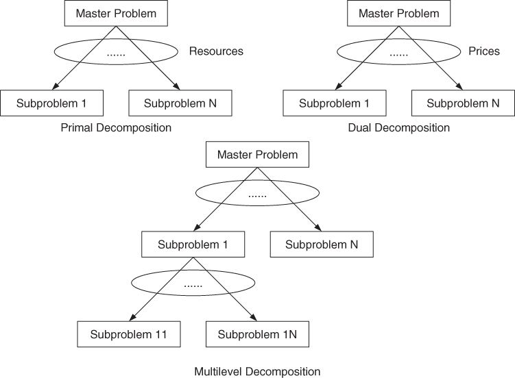
6.10.5.3 Cognitive Capability
Cognition is the key capability and foundation of cognitive cross-layer wireless networking system, which differentiates cognitive network from the traditional wireless networks. According to the Oxford English Dictionary, cognition is knowing, perceiving, or conceiving as an act [406]. Cognitive network is far more than cognitive radio which only covers layer one and layer two. In a cognitive network, all layers in all network nodes should have the capability of cognition. However, different layers or different nodes may have different levels of cognition. The upper layer should be more intelligent than the lower layer. Take spectrum usage as an example: spectrum sensing, spectrum decision, spectrum mobility, and spectrum sharing are the basic functions corresponding to cognition. Spectrum sensing is implemented in physical layer. Spectrum sensing obtains information of radio environment and provides it to the upper layer. The upper layer will make the decision which spectrum can be used for transmission. Spectrum mobility means cognitive radio users can move away from the licensed spectrum once the primary user occupies this spectrum again. If multiple cognitive radio users compete for the limited available spectrum, a spectrum sharing scheme should be set up to coordinate different users and different requirements.
Cognitive cross-layer wireless networking system is a highly dynamic system. Network topology, user behavior, and radio environment are rapidly changing. Cognition is an imperative capability for the networking system to work adaptively and intelligently. For example, if link stability is not maintained in harsh and dynamic RF environments or links are determined unsuitable for the following communication requirement, routing selection should be performed with consideration of spectrum occupancy, network topology, and user demand.
The abstract architecture of cognitive capability of a cognitive cross-layer wireless networking system is shown in Figure 6.3. There are three main modules to support cognition: cognitive network management, cognitive network monitoring, as well as knowledge representation and reasoning. Cognitive network management is the brain of cognitive cross-layer wireless networking system to determine network behavior intelligently. Network management refers to the activities, methods, procedures, and tools that relate to the operation, administration, maintenance, and provisioning of networking systems. Thus, the basic functions of cognitive network management are shown in Figure 6.4.
Figure 6.3 Abstract architecture of cognitive capability.
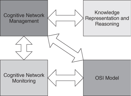
Figure 6.4 The basic functions of cognitive network management.
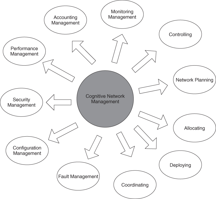
Cognitive network monitoring is to monitor the internal and external network data under the control of cognitive network management. These data can be spectrum sensing results, traffic information, buffer state information, channel state information, quality of connectivity, and so on. Recently, network tomography [534, 535] has been proposed to extract a network's internal characteristics using information derived from end point data. Originally, tomography is imaging by sections or sectioning, through the use of waves of energy, which is widely used in medical imaging, for example, Computerized Tomography. Network monitoring and inference have a strong resemblance to tomography [535] because the internal characteristics of an objective cannot be observed directly but can be inferred from external observations. In the current literature, two issues of network tomography have been addressed. One is link level parameter estimation from end-to-end path level traffic measurements [535]. The other is path level traffic intensity estimation based on link level traffic measurements [535]. The measurements of network tomography may be passive or active. Passive measurement will monitor the existing traffic flows. However, the temporal and spatial structure of the traffic process may make the measurement sample biased [535]. Active measurement will generate probe traffic into the network. If so, the probe traffic should not distort the network state for the existing traffic [535].
Knowledge representation and reasoning is to represent knowledge in a manner that facilitates inferencing from knowledge. Cognitive network can be treated as a wireless communication network augmented by this kind of knowledge plane that can span vertically over layers and horizontally across nodes [536]. There are at least two categories of functionalities in knowledge representation and reasoning. One is a representation of relevant knowledge. The other is a cognition loop using artificial intelligence, for example, machine learning technique. Besides, prediction is also the main function. Prediction results are very important information for cognitive network management to make the decision beforehand and to tackle the possible situations in the future. In this way, the operation of the networking system will be smooth and stable.
6.10.5.4 Potential Architectures
The key design of layering as optimization decomposition is that versatile network architectures can be rigorously obtained from the decomposition of an underlying cross-layer optimization problem [533].
Cross-layer routing and dynamic spectrum allocation in cognitive radio ad hoc networks have been studied in [537]. The main contribution in [537] is that a distributed and localized algorithm was derived for joint dynamic routing and spectrum allocation called ROSA for multihop cognitive radio networks. The cross-layer ROSA algorithm aims to maximize throughput through opportunistic routing, dynamic spectrum allocation, scheduling, and power control in a distributed fashion from transport layer to MAC layer. It is a good example to explore optimization decomposition for the network design.
Based on design philosophy and cognitive requirement, several network architectures will be presented using multilevel decomposition. As mentioned before, NUM is widely used as a design objective. QoS will be measured as NUM which implicitly covers many network performance metrics, for example, capacity, latency, security, stability, and so on. The cross-layer optimization issue is to maximize the sum of QoSs for different applications in the cognitive wireless networking system. Different applications or different services may have different weights in the design objective. This is the case in the context of multiobjective optimization. In the cognitive wireless networking system, there are many restrictions and limitations for the network operation, which will be formulated as the constraints in the optimization issue. These constraints at least include:
- network carrying capacity;
- limited power and limited computing capability in each network node;
- different spectral availabilities in different locations and at different times;
- interference tolerance;
- no interference to primary user;
- queue and buffer limitation.
Cognitive capability, for example, monitoring and inference, will be integrated into the cross-layer optimization issue. Because of the uncertainty introduced by cognition, the idea from robust optimization should be explored. Meanwhile, the overhead used for cognition will be formulated as the constraints for the cross-layer optimization issue. There are several potential architectures:
- Layered and distributed architecture. Vertical decomposition is performed to the cross-layer optimization issue first. Different functionalities are allocated to different layers to solve the optimization issue jointly. In transport layer, traffic control including congestion control and flow control are executed. Multipath routing and dynamic routing selection are exploited in network layer. Here, multipath routing can improve the robustness of data delivery in the dense deployment of network nodes [538]. Sophisticated scheduling, power control, and DSA are implemented in MAC layer for heterogeneous traffic. After vertical decomposition, horizontal decomposition will be carried out for each layer, respectively. Then, the same functionality will be distributed to the different network nodes.
- Distributed and layered architecture. The cross-layer optimization issue is divided into several subproblems by horizontal decomposition. Different subproblems will be solved by different network nodes. And then the task for each network node can be partitioned by vertical decomposition. There is an essential difference between the first architecture and the second architecture, because the first level decomposition plays a more important role for network architecture than the second level decomposition.
- Hybrid architecture. The cross-layer optimization issue will be decomposed completely by multilevel decomposition. Several different indecomposable subproblems will be assigned to one network node. The rule of assignment is that different nodes can share less information and use less coordination to solve these subproblems. This architecture breaks the standard layered architecture. Each node should have the capability of recomposing its functionalities flexibly and dynamically. Hybrid architecture is fully adaptive in the function level. Thus, in some situations, some nodes may have the light burden, and others may have heavy duty. Meanwhile, some nodes can even hibernate without any tasks for power saving. For dynamic routing selection in wireless sensor network, battery is the key issue for the sensor's life time. The sensor with less energy cannot be chosen as the next hop in the routing path even if the radio environment around this sensor is very suitable for wireless communication.
- Cluster based architecture. The cross-layer optimization issue is divided into several subproblems by horizontal decomposition. Different subproblems will be solved by different clusters in the wireless networking system. The cluster consists of a cluster head and several nodes around the cluster head. The cluster head is more powerful than any other node in the cluster. The cluster head is responsible for exchanging control information among different clusters and supervising other nodes in the cluster. Thus, the first level subproblem obtained by horizontal decomposition can be further partitioned. More functionalities will be allocated to the cluster head. The rest will be distributed to other nodes based on node capability and radio environment. The cluster based architecture is a good scheme to balance the central control and the distributed implementation.
- Mobility based architecture. The key point of this architecture is that the node, for example, unmanned aerial vehicle (UAV), has the mobile capability. The node can at least search for the available spectrum in different locations intelligently. The movement of nodes can change the existing network topology. However, this change is still under some level of control. Mobility based architecture can undoubtedly achieve autonomous network resiliency in the contested RF spectra. If the relay node is out of the communication range or there is no available spectrum for the relay node to use, this node can intelligently change its location to maintain the connectivity of wireless communication.
6.10.5.5 Physical Layer Consideration
In order to support the potential cognitive cross-layer wireless networking architectures and protocols, NC-OFDM will be exploited as the basic physical layer transmission technique. NC-OFDM is a noncontiguous version of OFDM with some unused subcarriers. OFDM is a highly recognized signal waveform for the current advanced wireless communication system, for example, 3G network, WiFi, WiMAX, and so on. DSA as well as OFDMA can be implemented based on NC-OFDM. Cognitive radio users can easily turn off some subcarriers which a primary user occupies and use other available subcarriers to transmit data.
How to efficiently implement NC-OFDM transceiver will be studied. At the transmitter, an FFT pruning algorithm and spectral shaping technique should be used to generate arbitrary NC-OFDM signaling. Because channel state information, primary user occupancy, and throughput requirement for cognitive radio users vary over time, an FFT pruning algorithm should be able to design an efficient FFT implementation every time conditions change [539]. Besides, PAPR issue should be taken into account in synthesizing NC-OFDM signaling from implementation consideration.
The other challenge for NC-OFDM transceiver is the synchronization at the receiver, especially for blind synchronization [540]. It is hard for cognitive radio to set up a dedicated control channel between the transmitter and the receiver. If the transmitter changes subcarriers to be used for data transmission, the receiver should have a way to detect or track this change, and jump to the correct subcarriers for receiving data without any control information aided from the transmitter. Meanwhile, due to the presence of the primary user, time domain correlation fails [540], even if the predetermined preamble is used. Thus, for blind synchronization, spectrum detection should be performed to find a new transmission first [540]. And then, the preamble is learned from those subcarriers for the new transmission. The regenerated preamble will be exploited to correlate with the following incoming signal [540]. Cognitive radio has no licensed spectrum. The reliable transmission between transceiver should be built as quickly as possible if some parts of spectra are available. Thus, it is worthwhile to implement a fast and effective synchronization scheme even at the cost of computational and implementation complexity.
MIMO will be also exploited in physical layer. MIMO technique or array signal processing can bring array gain, spatial diversity gain, and spatial multiplexing gain. Interference alignment [541] has been performed based on MIMO to explore degree of freedom in the spatial domain. Meanwhile, widely studied beamforming technique can be used together with routing selection and scheduling to improve spatial reuse [542]. Directional beam patterns can increase the communication range and reduce the interference to other directions.
6.11 Summary
In this chapter, optimization theory, especially convex optimization has been presented. Convex optimization is a powerful signal processing tool which can be exploited anywhere, for example, system control, machine learning, operation research, management, and so on. Linear programming, quadratic programming, geometric programming, Lagrange duality, optimization algorithm, robust optimization, and multiobjective optimization have been covered. This chapter can give readers the whole picture of optimization theory. Some examples have been shown in this chapter to help readers to understand how to use convex optimization to solve engineering problems or improve the system performances. If the engineering problems can be formulated as convex optimization problems, these problems will be solved without doubt. In cognitive radio network, optimization theory can be widely used for spectrum sensing [543, 544], cross-layer design, resource allocation, sensing disruption from adversary [545], and so on.