
CHAPTER OBJECTIVES
To understand the behavior of the demand for labor.
To explain, using a basic supply and demand model, how wages are determined.
To introduce some real-world considerations that modify the basic labor supply and demand model.
To describe the types and structure of unions, collective bargaining, and major legislation affecting labor.
To examine the distribution of income in the United States and some explanations for that distribution.
To define poverty, identify the poverty population in the United States, and discuss some government programs for alleviating poverty.

When we think about markets, we frequently think only of the markets in which goods and services are bought and sold: the discount malls we visit, our grocery stores, and the local shops that provide haircuts. But in a market economy, factors of production, like labor and capital equipment, are also bought and sold in markets. There are markets for nurses, book editors, high school math teachers, plumbers, architects, CEOs, and unskilled labor. As in product markets, substitutability and geography play an important role in defining factor markets. For example, an electrician in Denver will likely not compete with one in Houston for a job, but when a large corporation searches for a CEO, it will likely do an international search and consider people with a range of skills and experiences. And prices of factors, such as wages for labor, are the result of the degree of competitiveness in each labor market.
While there are markets for all of the factors of production, we will focus on labor markets in this chapter. The income from the sale of labor—wages, salaries, and such—is the largest single source of income in the U.S. economy: In 2011, labor income accounted for about 64 percent of all income.1
Since most of us will spend a lifetime in labor markets, learning about how they function is useful information. We begin this chapter with a look at a simple demand and supply model for wage determination and then explore the factors that cause many labor markets to deviate from this model. Since labor unions have been an important part of the U.S. economy, we will learn some basics about them as well. At the end of this chapter, we will learn about how income is distributed, how much people earn, and how we measure poverty in the United States.
LABOR MARKETS
In a market system, labor is bought and sold in the same way as goods and services: through the interaction of demand and supply. In the case of labor, however, businesses (and governments and nonprofits) are the buyers and individuals are the sellers.
The price of labor is called its wage. If someone works for a wage of $20 an hour, this is the price of that person's labor as well as the price the buyer is willing to pay.2
Wage
The price of labor.
Figure 15.1 gives a basic supply and demand model for determining the wage in a competitive labor market for workers who produce a particular service. The vertical axis of the figure gives wages per hour and the horizontal axis gives the quantity of labor demanded and supplied. In this particular market, the equilibrium wage is $15 an hour, and the number of workers employed is 800.
According to Figure 15.1, the demand curve for labor is downward sloping and the supply curve of labor is upward sloping: Buyers are willing to hire more labor as the wage falls, and more labor is offered in the market as the wage increases.
FIGURE 15.1 A Competitive Labor Market

There is a downward-sloping demand curve and an upward-sloping supply curve in a competitive market for labor.
The Demand for Labor
The demand for labor, or any other factor of production, is a derived demand: It is derived from, or depends on, the demand for the good or service the factor produces. Autoworkers have jobs because cars are demanded; grocery clerks are employed because people buy groceries; and the professors who teach your courses do so because students enroll in them.
Derived Demand
The demand for a factor of production depends on the demand for the good or service the factor produces.
The wage that a firm is willing to pay for a unit of labor is based on the dollar value of the labor's productivity to the firm. An employee whose daily product is valued at $150 will not be paid $175 per day. In fact, the company will not be willing to pay the employee over $150 a day. No firm can afford to hire at a wage rate greater than the employee's dollar contribution to the company. Baseball players with contracts in the tens of millions of dollars command this kind of money largely because of their expected contributions to their teams' earnings. Outstanding players attract fans who purchase tickets to games and increase revenues for the clubs.
As seen in Figure 15.1, the typical market demand curve for labor is downward sloping. This is because each individual firm's demand curve for labor is downward sloping: A firm is willing to hire more labor when the wage rate falls and less labor when the wage rate increases.3 If the amount a firm is willing to pay for labor is based on the dollar value of workers' productivity, then the downward-sloping demand curve indicates that the dollar value of workers' productivity falls as more labor is hired.
The declining value of labor's productivity as more labor is hired occurs for two reasons: (1) decreasing marginal productivity, and (2) the need to lower product price in order to sell more of a good or service.
TABLE 15.1 Total Product and Marginal Product of Labor for a Producer of Good X
As more workers are hired, after some point the Law of Diminishing Returns causes each additional worker's marginal product to decline.

Labor Demand and Productivity In discussing the pattern of short-run production costs in Chapter 12, the Law of Diminishing Returns was introduced. This law says that, beyond some point, the extra (marginal) product from adding successive units of a variable factor to a fixed factor falls. This concept applies to labor.
Law of Diminishing Returns
As additional units of a variable factor are added to a fixed factor, beyond some point the product from each additional unit of the variable factor decreases.
Table 15.1 provides an example of a hypothetical company varying the amount of labor it utilizes to produce good X. The second column of the table shows the total product that results when a specific number of workers is employed: For example, four workers together with the fixed factors produce 280 units of good X. The third column lists marginal product, which is the change in total product when one more unit of labor (the variable factor) is used. In Table 15.1, for example, the second worker has a marginal product of 80 units of good X (total product goes from 100 to 180 when the second worker is hired), and the fifth worker has a marginal product of 20 units (total product goes from 280 to 300 when the fifth worker is used).
Marginal Product
The change in total product when one more unit of a variable resource, such as labor, is utilized.
The most important point to observe in Table 15.1 is that marginal product declines as more workers are used.4 This decline is significant to the company employing the labor because it shows that, due to the Law of Diminishing Returns, each additional unit of labor produces less than the previous unit and is therefore worth less to the firm. This declining marginal productivity is reflected in the downward-sloping demand curve for labor.
Declining marginal productivity can be found in all work situations. Imagine the limited productivity of a baseball team's third, fourth, or fifth catcher. A restaurant will find that at some point the marginal productivity of its additional servers declines as more are employed, and a high school that hires several assistant principals may find each successive one adding less to total product than the one before.
Labor Demand and Product Price The second reason for the declining value of labor's productivity and the resulting downward-sloping labor demand curve is the demand for the good or service the labor is producing. In all market situations except pure competition, firms face downward-sloping demand curves for their products: Consumers will increase their purchases of a company's product only if its price falls. This downward-sloping demand curve for the good or service that labor produces causes the value of labor's productivity to decrease, since the increased output resulting from employing more workers can only be sold at lower prices. Thus, additional units of labor are worth less to the company because the product they produce is sold for less.
TABLE 15.2 A Good X Producer's Total Product and Price per Unit
A firm facing a downward-sloping demand curve for its product can sell the increased output that results from hiring more workers only if it lowers the price.

To illustrate this point, Table 15.2 gives the total product information from Table 15.1 for the producer of good X and adds a third column listing the prices at which good X can be sold. The price and total product columns reflect the inverse relationship between price and quantity demanded: If the company intends to sell more of its product, it must lower the price. However, lowering the product's price decreases the value of what labor produces.
Combining Declining Marginal Productivity and Declining Product Price The demand curve for labor is downward sloping because the marginal productivity of additional units of labor decreases and because the value of additional production is lowered by the decline in price necessary to sell the product. In other words, the Law of Diminishing Returns and the Law of Demand combine to determine the value of labor.
The effects of declining marginal productivity and decreasing product price can be combined to determine what each unit of labor is worth to a firm. This in turn determines the wage rate a firm is willing to pay. Returning to the good X example, Table 15.3 adds two columns to those given in Table 15.2 in order to determine the wage rate the producer of good X is willing to pay.
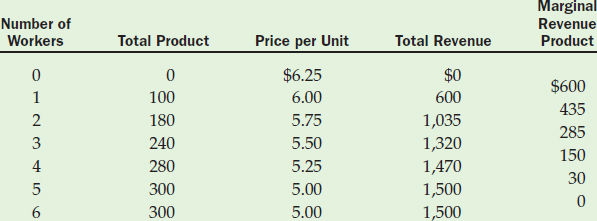
The fourth column of Table 15.3 gives the total revenue when various amounts of good X are sold. (Remember: Total revenue is price times quantity.) For example, with a total production of 240 units that can be sold for $5.50 each, total revenue is $1,320 (240 × $5.50).
The last column of Table 15.3 gives marginal revenue product, which is the change in total revenue that results from the sale of output produced when one more unit of labor is utilized.5 When one worker is hired, 100 units of good X are produced and sold for $6 each, bringing in $600 for the company. Since the total revenue with no workers is $0, the marginal revenue product of the first worker is $600. When a second worker is employed, 180 units of output are produced and sold for $5.75 each, creating a total revenue of $1,035. Thus, when the second worker is utilized, the company's total revenue increases from $600 to $1,035, or the marginal revenue product of the second worker is $435. For the third unit of labor, the marginal revenue product is $285 because total revenue increases from $1,035 to $1,320. The marginal revenue product of the fourth worker is $150 and of the fifth worker is $30.
Marginal Revenue Product
The change in total revenue that results from the sale of output produced when one more unit of a variable factor, such as labor, is utilized.
TABLE 15.3 A Good X Producer's Total Product, Price, Total Revenue, and Marginal Revenue Product
Marginal revenue product is the change in total revenue that results from the sale of output produced when one more unit of a variable factor, such as labor, is utilized.
Marginal revenue product is important because it establishes the firm's demand curve for labor. In the example in Table 15.3, this firm would not hire any labor if the wages were above $600. In this case, the wage paid would be greater than the extra revenue created by the production of any worker. The producer would, however, be willing to hire one worker at a wage of $600. At $600, the first worker's contribution (marginal revenue product) equals the wage.
The wage would need to fall to $435, the marginal revenue product of the second worker, before the producer would hire two units of labor. At any wage higher than $435, the second worker's contribution to the firm's revenue would be less than the wage. For three units of labor to be employed, the wage would have to fall to $285, the marginal revenue product of the third worker. Four workers would be demanded at a wage of $150 and five at $30.6
When the wages and the amount of labor the good X producer is willing to hire at each of those wages are plotted in a graph, the firm's demand curve for labor results. This is given in Figure 15.2. Notice that the wage is equal to the marginal revenue product of labor at each point on the demand curve. Test Your Understanding, “A Small Business Determines Its Demand for Employees,” provides an opportunity to calculate some of these demand-related numbers and to derive a labor demand curve.
Demand Curve for Labor
Downward-sloping curve showing the amount of labor demanded at different wage rates; based on the marginal revenue product of labor.
The Supply of Labor
In a typical labor market there is a direct relationship between wages and the quantity of labor supplied, causing the supply curve of labor to slope upward like that given in Figure 15.3. This relationship implies that less labor will be attracted to a market at a lower wage than at a higher wage. In Figure 15.3, for example, 300 people are willing to work in this labor market for $8.00 per hour, but 700 want to work for $11.50 per hour.
Supply Curve of Labor
Upward-sloping curve showing the amount of labor supplied at different wage rates.
FIGURE 15.2 A Firm's Demand Curve for Good X Workers

A firm's demand curve for labor is based on the marginal revenue product of labor, which declines as additional workers are hired.
In labor markets, money may be only part of the consideration in seeking a job. Many important factors other than wage or salary influence the supply of labor: location preferences, psychological rewards, long-term work objectives, and other nonwage considerations. Think about your current job or one you have held in the past. What nonwage factors influenced you in taking this job? How do nonwage factors contribute to the lack of job applicants to pick up trash in July in cities with extremely high temperatures? Or, what might cause a teenager to want a job at Starbucks or Macy's while not even considering a job at a fast-food restaurant that pays the same wage?
FIGURE 15.3 Supply Curve of Labor

A typical upward-sloping labor supply curve indicates that a direct relationship exists between wage rates and the quantity of labor supplied in a market.
TEST YOUR UNDERSTANDING
 A SMALL BUSINESS DETERMINES ITS DEMAND FOR EMPLOYEES
Suppose you plan to start a small business that will label and stuff envelopes for other small businesses, charitable fund raisers, and political candidates. Since your biggest cost will be for employees to do the actual labeling and stuffing, you are very concerned about determining the hourly wage you would be willing to pay.
Assume that the information given in the following tables is from a study done for a company similar to the one you plan to start. This information serves as the basis for determining the wages you would be willing to pay and how many employees you would be willing to hire at each wage rate.

The hourly total product (envelopes) that can be produced with different numbers of workers is shown in Table 1. Determine the hourly marginal product of each additional worker and answer Question 1.
- At what number of workers does the Law of Diminishing Returns take effect?_________
Table 2 gives the price for stuffing and labeling each quantity of envelopes: If your output is 1,500 envelopes per hour, you can charge 4¢ ($0.04) per envelope and sell that output. But if you raise your output to 2,250 per hour, you must lower your price to 3¢ ($0.03) per envelope to sell your services to more buyers.

Determine the hourly total revenue and the hourly marginal revenue product per worker from the information in Table 2. Put these numbers in Table 3 and answer Questions 2 through 4.

- What is the highest hourly wage that you would be willing to pay?___________________
- What wage would you be willing to pay to hire enough workers to label and stuff 1,500 envelopes per hour?_____________________
- Suppose you have enough demand for your services to label and stuff 2,250 envelopes per hour at 3¢ each, but the minimum wage is $7.50. Would you lower your price to 3¢?__________________
Based on the numbers in Table 3, complete the demand schedule for employees in Table 4 and draw the resulting demand curve for labor in the graph provided.
| Number of Workers Demanded | Wage Rate |
| 1 | _____ |
| 2 | _____ |
| 3 | _____ |
| 4 | _____ |
| 5 | _____ |

Answers can be found at the back of the book.
Location is an important nonwage influence on the supply of labor in some markets, particularly small towns with few employers where workers face limited job choices. Rather than relocate to earn a higher income, some people choose to stay in their familiar surroundings and work at a lower wage. When there are many job opportunities in an area, workers can be more selective and sensitive to wage rates. National chain stores, such as Wal-Mart, may be able to pay lower wages in areas with little competition for unskilled labor than in large, populated metropolitan areas.
Many people seek a job that is psychologically rewarding or that gives them “psychic” income: Prestige, a sense of accomplishment, or freedom from supervision may induce a person to work for a lower wage. Someone with an advanced degree in international management, for example, might prefer to teach and receive a smaller salary from a prestigious university than to work for a higher salary from a large corporation. A freelance writer might sell an essay for little money to a highly regarded magazine because of the sense of accomplishment from having an article in that particular publication.
The possibility of long-term gain can also influence the supply of labor. A college graduate may take a position with an employer at a lower salary than that offered by other employers because the potential for future advancement is great or because the job will look good on a resume. Other factors affecting supply include job security; the safety, cleanliness, and working conditions on a job; the degree of skill or formal training required; and flexibility in scheduling work.
Changes in Labor Demand and Supply
In any labor market, changes can occur that will cause labor demand and/or supply to increase or decrease and the demand and/or supply curves for labor to shift to the right or left. When these changes occur, the equilibrium wage and amount of labor hired are affected in the same way that equilibrium price and quantity are affected when demand and/or supply shift in an output market. An increase in the demand for labor, for example, causes the demand curve to shift to the right, resulting in an increase in both the equilibrium wage rate and the number of workers employed. This is illustrated in Figure 15.4, which demonstrates graphically the effect of an increase in the demand for labor from D1 to D2 in a competitive labor market. As demand increases, the equilibrium wage rate rises from W1 to W2, and the number of workers employed increases from Q1 to Q2.
FIGURE 15.4 Effect of an Increase in Demand in a Labor Market

An increase in the demand for labor causes both the equilibrium wage rate and quantity of workers employed to increase.
Changes in Labor Demand There are many factors that can cause a demand curve for labor to shift to the right or left: changes in the prices of substitute inputs, technological change, and changes in the demand for the good or service the labor is producing are just a few. Let's consider each of these.
Businesses are always looking for cheaper methods of production to improve profits. If they can find and use a cheaper input, the demand for the more expensive input will decrease and its demand curve will shift to the left while the demand for the cheaper input will increase and its demand curve will shift to the right. The search for cheaper inputs has affected many labor markets. Automobile companies have turned to robotics in their plants, causing the demand for labor to fall, and lower labor costs in many foreign countries have led to the closing of U.S. manufacturing plants. For example, in September 2008, Hanesbrands, maker of Hanes and Champion apparel, announced that it was closing plants and cutting 8,100 staffers as it consolidated into fewer, larger plants in lower-cost countries, particularly in Asia. In 2010, BP announced the closing of its solar-panel manufacturing plant and the laying off over 300 workers in Frederick, Maryland, as BP continued to move its solar business to countries like China and India.7
Technological change has an important impact on the demand for labor. The widening use of computer-based information, programs, and storage systems has increased the demand for people with technology-related skills, while at the same time decreasing the demand for many other types of labor. Today most businesses and organizations employ a staff of skilled hardware and software technicians. The emergence of programs such as Turbo Tax, which allows individuals to prepare and file income taxes online, has influenced other fields such as accounting, where fewer “humans” are needed. Even grocery stores are eliminating labor because of computerized self-checkouts, and trash trucks need fewer workers because of mechanized lifts.
APPLICATION 15.1
 GO GREEN
Today the concern over sustainability is the classic acknowledgement of the basic principle of scarcity at the root of economics: scarce resources with unlimited wants and needs. Apprehension over the limits of basic resources necessary to sustain life—clean air and water and energy sources—has given rise to a movement that focuses on policies and actions to address these concerns.
Our language now includes words and phrases that have a different meaning than they did in our parents' and grandparents' generations: sustainability, recycling, wind farms, and hybrids to name a few. And, adding to that lexicon is the new usage of green—green products, green building, green jobs, and more.
There is focus today on a new green economy with its positive impact on the creation of green jobs and green careers. Job seekers are being directed toward employment opportunities that are arising from our concerns for sustainability. There are websites that list green job opportunities and recently Forbes identified “The Top 10 Cities for Green Jobs.”
So what exactly is a green job? How do we define that sector of the economy? Recently, the U.S. Department of Labor's Bureau of Labor Statistics (BLS) began to collect data on green jobs in order to analyze the impact that sustainability concerns are having on economic activity. In doing so, the BLS has developed an “official” definition. Green jobs are:
- jobs in businesses that produce goods or provide services that benefit the environment or conserve natural resources; and
- jobs in which workers' duties involve making their establishment's production processes more environmentally friendly or use fewer natural resources.
According to the BLS, green jobs range from those associated with producing energy from sources like wind and solid waste to those that reduce the release of toxic compounds to jobs that increase public awareness of environmental issues or introduce technologies that conserve natural resources.
While we struggle to assess and measure the strength of the green economy and the jobs it is creating, we continue to aspire toward the goals of a cleaner, better, healthier world. And those aspirations show up in the continued emphasis on green activities whether they are formally measured or not. All one needs to do is google “green jobs” and a plethora of websites that direct job seekers toward a variety of positions pops up.
Experienced workers and new college graduates will find firms looking for environmental engineers, landscape designers who can create rain gardens, energy consultants, solar sales representatives, urban farmers, and more. Even in traditional fields like marketing and communications, there are jobs with a green emphasis. And, the LEED certification (Leadership in Energy and Environmental Design) developed by the U.S. Green Building Council is encouraging professionals in architecture and construction to incorporate the knowledge and practice of green design and building into their projects.
Sources: Jacquelyn Smith, “The Top 10 Cities For Green Jobs,” www.forbes.com; U.S. Green Building Council, “What LEED is,” www.usgbc.org; U.S. Department of Labor, Bureau of Labor Statistics, “Measuring Green Jobs,” www.bls.gov/green/.
Finally, a change in the demand for the good or service that a type of labor is producing may change the demand for that labor. When the demand for new single family housing increases, developers and construction companies increase their production, causing the demand curve for construction workers to shift to the right. In 2008 and 2009, as the economy fell into a serious recession, the demand for cars and trucks took a serious hit. The decline was so severe that several U.S. auto companies went to Congress seeking a financial bailout to survive. During this period the automobile companies were shutting down production lines as their inventories swelled, and the demand for auto workers clearly went on the decline.
Application 15.1, “Go Green,” deals with the rise in new jobs and careers coming from the emphasis on creating products and services associated with sustainability of the earth's limited resources. The movement toward “greening” is affecting a large number of labor markets from various types of engineers to environmental consultants.
Changes in Labor Supply We can identify a number of factors that cause the supply of workers in a labor market to change and the supply curve to shift to the right or left. These include, among others, changes in economic conditions, demographic trends, expectations, and immigration.
Some labor markets are affected by the state of the economy, such as those for low-paying, unskilled jobs in businesses like fast-food restaurants, retail stores, and lawn care. With healthy economic conditions, the supply of workers in these labor markets decreases as people find better-paying jobs. When the economy in general or in a region falls into a recession and workers are laid off—especially for long periods of time—those laid-off workers, as well as household members who now need to supplement household income, enter these labor markets and increase supply.
Demographic trends also affect labor supply. For example, when the teenage population increases, firms that typically hire from this age group, such as mall shops, experience an increase in labor supply. Also, with the trend toward early retirement there is a drop in supply in some labor markets with full-time jobs and a movement of workers into labor markets where part-time employment is available.
The expectation of future job prospects influences the supply curve in some labor markets. College students, for example, tend to select majors that are perceived as providing good employment opportunities. When the number of teaching positions in secondary and elementary schools increases, for example, the supply curve of new teachers shifts to the right as more students major in education, and when getting a good job in investment banking or other financial services appears less likely, the supply curve of students with majors in finance shifts to the left.
Many other factors cause labor supply to increase or decrease. For example, changes in immigration laws and the extent to which illegal immigrants are returned to their home countries affect several labor markets, and the number of students accepted into medical and law schools influences the supply of labor in those markets.
Changes in Labor Demand and Supply, and Changes in Quantity Demanded and Supplied The distinction made in Chapter 3 between a change in demand or supply and a change in quantity demanded or supplied applies to labor demand and supply. A change in labor demand or supply refers to a shift of the entire labor demand or supply curve to the right or left as a result of changes in nonwage factors, such as the prices of substitute inputs, technology, product demand, economic conditions, and expectations about future job prospects. A change in the quantity of labor demanded or supplied occurs only as a result of a change in the price (wage) of labor. A change in quantity demanded or supplied is represented by a movement from one wage–quantity combination to another along a labor demand or supply curve: The curve itself does not change.
Change in Labor Demand or Supply
A shift in the demand or supply curve for labor caused by changes in nonwage factors.
Change in the Quantity of Labor Demanded or Supplied
A change in the amount of labor demanded or supplied that occurs when wages change; a movement along the demand or supply curve.
Modifications of the Labor Demand and Supply Model
The labor market model introduced in Figure 15.1 at the beginning of the chapter is a useful starting point for analyzing how wages are determined through the forces of supply and demand. But, just as there are imperfections in output markets, there are certain factors at work in real-world labor markets that go beyond what is explained in the simple supply and demand model and that impact the determination of wages and the amount of labor employed. Three of these factors—wage rigidities, legal considerations, and unequal bargaining power—merit special consideration.
Wage Rigidities In a labor market such as that in Figure 15.1, a decrease in the demand for labor would shift the demand curve to the left, causing fewer workers to be hired and the equilibrium wage to fall. In reality, a decrease in the demand for labor will most likely cause employment to drop, but not money wages.8 Firms with a need for fewer workers usually respond by laying off workers rather than by lowering their wages. On the supply side, contrary to the operation of the simple model, an increase in the number of workers in a market (a shift of the supply curve to the right) will also likely not lower the money wage. Thus, money wages tend to adjust upward but not downward to changing labor market conditions.
There are several reasons why money wages tend not to fall: Some workers are earning the minimum wage and by law can be paid no less; an employer may be bound by a labor agreement that sets wages; and it may be in the worker's best interest to be laid off rather than take a cut in pay. A laid-off worker may become eligible for unemployment compensation, can use the idle time to find another job, and will not be acknowledging a willingness to work for less. Also, an employer might believe that better long-term employee relationships can be maintained by laying off workers for a short period of time rather than by asking workers to accept a lower wage.
Legal Considerations Labor markets are affected by legislation that influences wages and the demand for and supply of labor. The most obvious legislation is the minimum wage law. By setting minimum hourly earnings, this law can override supply and demand by not allowing wages to fall to equilibrium. Figure 15.5 gives the federal minimum wage over time from $0.25 per hour when established in 1938, to $7.25 per hour set in 2009.
Minimum Wage Law
Legislation specifying the lowest hourly earnings that an employee can be paid.
Figure 15.6 shows the influence of the minimum wage law on a labor market. The equilibrium wage in Figure 15.6 is $6.00 per hour, and the equilibrium employment is 2,200 workers. If the government establishes a minimum wage above the equilibrium—say, $7.25 per hour—employers will want to hire only 1,800 workers, but 2,400 workers will be available. As a result, a surplus of 600 workers will develop in the market. Many critics of minimum wage legislation point out that it causes unemployment in some labor markets. The graphics in Figure 15.6 suggest this may be so.
Some legislation can change the demand for labor. For example, the minimum wage law may reduce the demand for a type of labor if the increased wage makes it cheaper to use a piece of machinery to do the job. Rules, such as those of the Occupational Safety and Health Administration (OSHA) that specify safety and working conditions, may affect employers' costs of using labor and, in turn, their demand for labor. There are also laws relating to the hiring of specific groups in the labor force, such as women and minorities, that influence labor demand.
The supply of labor is also affected by various laws. Licensing and certification requirements for physicians, occupational therapists, teachers, and others have an impact on the supply of labor. Various federal, state, and local laws that influence immigration levels, forbid the use of illegal foreign workers, and impose large penalties on employers who violate these laws have a major impact on the supply of labor in some markets, especially those for unskilled workers. Laws limiting the amount people can earn while on Social Security, laws pertaining to unemployment compensation, and child labor laws also affect the supply of labor.
FIGURE 15.5 The Federal Minimum Wage

Over the years, the minimum wage has been raised many times from its original $0.25.
FIGURE 15.6 Effect of a Minimum Wage on a Labor Market

When the equilibrium wage in a labor market is lower than the minimum wage, the minimum wage prevails, and a surplus of workers results in that market.
Unequal Bargaining Power The equilibrium wage of $15 in the labor market in Figure 15.1 was determined by employers and employees with equal bargaining power. In many markets this is not the case.
If bargaining power is on the side of the employer, the wage will likely be below that set when both parties are of equal strength. For example, workers living in a town with one major employer may be paid a lower wage than if there were several firms competing for their services. And, years ago before free agency status for athletes, studies showed that their salaries were much lower. In general, the fewer the alternative employers from which workers can choose, the weaker the workers' bargaining power.
If bargaining strength is on the side of labor suppliers, the wage will likely be above that set when buyers and sellers have equal power. In general, the greater the suppliers' control over the labor available to a particular employer, the greater their ability to raise wages above the competitive level. One method used by workers to raise wages has been unionization. In addition, exceptional abilities and skills, such as those of some network news anchors or sports personalities, provide greater control over their supply of labor.
LABOR UNIONS
A labor union is an organization of workers that bargains with management on its members' behalf. Usually unions represent their members in negotiations for wages, working conditions, fringe benefits, rules relating to seniority, layoffs and firings, and other matters. Unions in the United States are primarily economic in their focus, although they may engage in some political activity.
Labor Union
An organization of workers that bargains in its members' behalf with management on wages, working conditions, fringe benefits, and other work-related issues.
Types of Unions and Union Membership
The percent of the labor force belonging to unions has not been stable over the years and in recent decades the power and influence of unions have declined. In 1983, 20.1 percent of all wage and salary employees belonged to unions, but since then membership has fallen. By 2011, only 11.8 percent of these workers were unionized. And, perhaps surprisingly, a much larger percentage of public sector workers are unionized than are private sector workers: About 37 percent of government workers were unionized in 2011 as compared to 6.9 percent of private sector workers.9
The erosion of union membership and power has stemmed from many sources: an antiunion political climate; growth in service sector jobs where unionism has not had a strong presence; the decline in blue-collar manufacturing jobs where unions have been relatively successful; expanded government regulation of working conditions; and retirements of union workers who were strong advocates for the union movement.
Labor unions fall into two categories: craft unions and industrial unions. Craft union membership is made up of workers who have specific skills, such as bricklaying or plumbing. So, for example, bricklayers on a particular construction job would be represented by one union and plumbers on the same job by another.
Craft Union
A union that represents workers with a specific skill or craft.
A craft union may restrict membership through the completion of an apprenticeship program or some other requirement. Setting such conditions gives the union some control over the supply of workers, which helps raise its members' wages and fringe benefits. A simple supply and demand model for wage determination indicates that any action that restricts supply (shifts the supply curve to the left) results in a higher wage rate. For example, Figure 15.7 shows that a decrease in the supply of labor from S1 to S2 leads to an increase in the wage rate from W1 to W2. Notice also another important result. This action reduces employment: in this case from Q1 to Q2.
FIGURE 15.7 Restricting Supply in a Labor Market

A craft union can obtain higher wages for its members by limiting the supply of labor, which is shown by a shift of the supply curve to the left from S1 to S2.
An industrial union, rather than limiting itself to workers with a single skill, represents all workers in a specific industry. For example, workers performing different jobs in the automobile industry may be represented by the United Auto Workers, and communications workers performing different jobs may be represented by a single union. When it comes to membership, industrial unions are broader in their focus than craft unions.
Industrial Union
A union that represents all workers in a specific industry, regardless of the type of job performed.
A union, whether craft or industrial, is typically headed by a national or international organization that operates on behalf of all the members. Below this headquarters organization are individual “locals” to which the members belong. In some cases, such as the musicians' and other craft unions, members who work for different employers in a particular area belong to the same local. In other cases, such as the autoworkers' and other industrial unions, a local represents members working in a single plant or for a single employer.
Collective Bargaining
With unions, the process of wage determination is more complicated than the simple interaction of market supply and demand since a union represents the suppliers of labor and management represents the buyer of labor. Here the impersonal forces of the market are replaced by negotiations between union and management representatives seeking to reach an agreement on wages, fringe benefits, and other aspects of a labor contract. This process in which a union negotiates a contract on behalf of its members is referred to as collective bargaining.
Collective Bargaining
The process through which a union and management negotiate a labor contract.
Union and management negotiations are primarily about economic issues: wages, job security, payments for insurance, and such. But the actual bargaining process itself is largely political: Negotiation involves a give-and-take process where each side tries to gain the most of what it seeks while giving up the least. The terms of a negotiated contract depend in large part on the relative bargaining ability and strength of the participating parties.
If the parties to a negotiation fail to agree on the terms of a contract, a union may go on strike against the employer. When on strike, union members stop working and often set up a picket line that other workers may refuse to cross. The purpose of the strike is to bring economic pressure on the employer to return to the bargaining table and draft an agreement acceptable to the union. In recent years little labor time has been lost due to strikes. In 2010, for example, less than 0.005 percent of estimated working time was lost because of work stoppages.10
Strike
Work stoppage by union members.
Collective Bargaining and the Law
Over the years, we have created a large body of laws concerning the rights and responsibilities of labor unions in collective bargaining and related matters. Two laws have been especially important: the National Labor Relations Act of 1935 and the Labor Management Relations Act, better known as the Taft-Hartley Act, of 1947.
Passed in the depths of the Depression, the National Labor Relations Act (also called the Wagner Act) specifically gives workers the right to organize and bargain collectively, to choose who will represent them in their collective bargaining, and to carry out “concerted activities” for pro-labor purposes. The law also defines certain actions by employers, such as discrimination against employees because they belong to a union, as unfair labor practices. The National Labor Relations Board (NLRB), which hears complaints about unfair labor practices and can order that those practices cease and be remedied, was also established by the act.11
National Labor Relations Act (Wagner Act)
Legislation supportive of unions; permits and strengthens collective bargaining.
National Labor Relations Board (NLRB)
Hears complaints on unfair labor practices and orders remedies where appropriate.
The Taft-Hartley Act of 1947, which became law in a troublesome year for work stoppages, is generally less supportive of organized labor. Under certain circumstances the Taft-Hartley Act gives workers the right to not join a union or otherwise engage in organized labor activities. Section 14(b) of the law says that union membership cannot be a condition of employment in states that have passed laws to that effect. This is better known as the “right to work” issue, and state laws prohibiting union membership as a condition of employment are called right to work laws. With right to work laws, a union's ability to control the supply of labor is diminished, and the union's bargaining strength is weakened. In 2010, 23 states had right to work laws.12
Taft-Hartley Act
Legislation that contains several provisions limiting union activities.
Right to Work Laws
State laws prohibiting union membership as a condition of employment.
The Taft-Hartley Act also allows the president of the United States to impose an 80-day “cooling-off period” during which a particular strike or lockout (where an employer prevents laborers from entering a work site) cannot occur if, in the president's opinion, the work stoppage is a threat to the national interest. If, after 80 days, the situation leading to the strike or lockout is not corrected, the ban is lifted, and the work stoppage can continue.13
THE DISTRIBUTION OF INCOME
In any economy, there are always questions about income. How much does the average person make? How is income divided—are there many or a few rich or poor? The distribution of income refers to the way income is divided among the members of society. If the distribution of income to individuals were perfectly equal, everyone would receive the same amount. But income is not divided equally: Some households are better or worse off than others; and at the extremes, some are very rich and others are very poor.
Distribution of Income
The way income is divided among the members of society.
We can see how income is distributed in the United States in Table 15.4. The left-hand column of the table divides households into five groups—each representing 20 percent of all households—ranked according to the amount of income each group received. The lowest group represents the 20 percent of all households that received the lowest incomes, and the highest group is the 20 percent that received the largest incomes. The right-hand column of the table gives the percentage of total income that went to each of the five groups in 2011.
With an equal distribution of income among households, each of the five groups would receive 20 percent of the total. However, in 2010 the lowest 20 percent received 3.2 percent of total income, while the highest 20 percent of households claimed 51.1 percent. Not shown in the table, the top 5 percent received 22.3 percent of total income.14
Over the years, journalists and others have watched the release of these annual quintile data to determine the direction of shares of income. Since 1970 there has been a slow and gradual change in the shares: the rich are getting richer, the poor are getting poorer, and the middle class is slowly shrinking. With the recession and financial crisis that began in 2008, a spotlight has been put on these data. Notice now that the top 20 percent of households earn over 50 percent of the income generated and that the lowest 60 percent of all households earn just over 25 percent of all income generated. Interest has also been sparked in knowing just how much money top income earners make and the salaries of corporate CEOs are popular public information. Today there is reference to the amount of income generated by the top 1 percent, and since the fall of 2011 “Occupy Wall Street” protests have sprung up around the country, partly to bring attention to income shares.15
TABLE 15.4 Income Distribution among Households
Income is not distributed evenly among households in the United States. In 2011 the poorest one-fifth of U.S. households received 3.2 percent of total income while the richest one-fifth received 51.1 percent of the total.

Source: U.S. Census Bureau, Table H-2, www.census.gov/hhes/www/income.
Some members of society are more likely than others to be at the lower or higher end of the distribution of income. In Chapter 10 it was noted that, on average, households with certain characteristics tend to earn more than other households. For example, households headed by a married couple typically earn more than households headed by a single female, and households headed by a college graduate fare better than those headed by an individual with less education.16
Differences in Income
Why is income in the United States distributed as it is? Why do some people receive a large annual income while others do not? Several explanations merit discussion.
Resource Ownership Most income depends on the quality and quantity of productive resources that individuals own and the uses to which those resources are put. People with highly productive or many resources stand to earn more money than those who own less productive or fewer resources. An outstanding athlete or top-rated chef earns more than others with less impressive performances; the owners of fertile farmland in the heart of Illinois earn more income per acre from the production of crops than the owners of less fertile farmland in the hills of western Pennsylvania; and a family with a ranch, an apartment complex, and a fleet of rental trucks is going to have a higher income than one whose sole income source is the labor of an unskilled household head.
Sometimes resource ownership comes from inheritance. Income can be generated from the ownership of real estate, securities, or other assets passed on through a will or trust.
Education and Experience The case can be made that nothing beats education as a way of improving a person's lifetime earnings. We saw the data in Chapter 10 that show a direct relationship between annual household income and years of education. Table 15.5 provides more detailed information about average weekly incomes for people whose education levels range from less than a high school diploma through a professional degree like an MD or a law degree. The data in the table strikingly demonstrate the importance of education: In 2011 a person with a professional degree was earning about 3.4 times as much as a person with less than a high school diploma.
TABLE 15.5 Levels of Education and Income
Education has a strong positive influence on a person's income.
| Education Level | Average Weekly Earnings in 2011 |
| Professional degree | $1,665 |
| Doctoral degree | 1,551 |
| Master's degree | 1,263 |
| Bachelor's degree | 1,053 |
| Associate degree | 768 |
| Some college, no degree | 719 |
| High school graduate | 638 |
| Less than high school diploma | 451 |
Source: U.S. Department of Labor, Bureau of Labor Statistics, Employment Projections, “Education Pays,” http://www.bls.gov/emp/ep_chart_001.htm.
There is also a case to be made for experience, which includes not only work at a job, but training, additional coursework, the reading of work-related articles and books, and other activities over time. It has been shown that the financial benefit of experience is higher for those with more education.17 Presumably, individuals with jobs that require a higher degree also invest more in additional training. The expenditure of time, effort, and money by a physician who must keep up with licensing requirements, continuing education, and professional readings is typically higher than that by someone in an unskilled labor position.
The expenditures of time, effort, and money to gain an education and improve a person's productivity are called human capital investments. Just as a business may invest in machinery and equipment, human beings can and do spend money and time improving their own productive capabilities—both intellectual and physical. Human capital investments include not only learning-related expenditures but also spending on health care, fitness, and other related programs. As the world becomes “flatter” and we compete in a more global environment, there is increased recognition that knowledge-based economies are important for sustained economic growth.
Human Capital Investment
An expenditure to improve a person's productivity.
Application 15.2, “Making the Most of Intellectual Capital,” discusses the transition in the United States from an economy that was focused on industrial work and skills to a more sophisticated economy dependent on brain power, or intellectual capital.
APPLICATION 15.2
MAKING THE MOST OF INTELLECTUAL CAPITAL
Knowledge didn't fuel America's economy in the past. The Industrial Age thrived on man's mastery over machine. Most work required steady hands to operate factory equipment and minds geared to such repetitive tasks as measuring and counting…. Over the course of workers' careers, jobs changed little, so talents acquired in youth often served until retirement. Lifetime learning didn't matter all that much.
America has left the Industrial Age behind. Factory work is increasingly being performed in other countries; much of what remains in the United States is highly technical, relying more on sharp minds than nimble hands.
Postindustrial nations are shifting workers to more sophisticated jobs that require analytical intelligence, imagination and creativity, and the ability to interact with others. The work relies on brains rather than brawn…. Equally important, these skills have to be kept sharp in a world of rapidly changing tastes and technology. We can't just get a good education while young and expect it to suffice for an entire career.
The transformation of the way we work gives intellectual capital precedence over the physical capital that once drove the U.S. economy. Both kinds of capital make us richer, but they differ in important ways.
Physical capital grows when businesses invest in buildings, machinery and other productive assets. These are largely management decisions, and the process usually takes just a few months or years. To expand intellectual capital, we invest in human beings over decades—from learning the ABCs in preschool to mastering the latest computer programs at the office.
Companies make important contributions to creating intellectual capital, but workers must assume a large part of the responsibility. No one can learn for us. We have to supply the effort to develop our skills.
Knowledge is ultimately the property of the employee…. Workers take it with them when they switch jobs, a factor that limits companies' ability to capture the benefits of investing in human capital. As a result, workers can't count on employers to provide all the training they'll need. They must be active participants in their own education, engaging in lifetime learning on their own.
Source: “Making the Most of Intellectual Capital,” Federal Reserve Bank of Dallas, 2004 Annual Report, pp. 13–14.
Discrimination Workers experience discrimination when they are treated unequally in a labor market because they are placed in a category and judged on the basis of the employer's perception of that category, rather than on the basis of their skills or merit. In the United States, concern over discrimination has centered mainly on the labor market experiences of nonwhite as compared to white workers, female as compared to male workers, and older as compared to prime-age workers. But discrimination can be based on any type of categorical distinction, such as religious or political preference or ethnic origin. Typically, the discriminated-against worker receives a lower wage or may have fewer job choices or advancement opportunities.
Discrimination
Unequal treatment in a labor market because of an employer's perception of a category to which a worker belongs.
The effects of discrimination on income can also be indirect. Unequal access to good housing, medical care, or educational opportunities might lead to smaller or less productive human capital investments, which in turn can result in lower incomes.
Poverty
The income distribution data in Table 15.4 show that, in 2011, the lowest 20 percent of all households received only 3.2 percent of total income, and the next lowest 20 percent received only 8.4 percent. Are these households considered to be the “poor” in our society?
Each of us has a different concept of poverty, or what is meant by poor. What someone living in luxury considers to be poor may be different from what the average income earner thinks is poor. Someone who drives an expensive new car may think a person who drives an old, obviously used car is poor. Someone who drives an old used car may view as poor a person who cannot afford a car at all.
TABLE 15.6 Poverty Levels for Families and Individuals
Poverty levels vary according to family size and age of the head of the household. They indicate the annual money income that must be received to be considered not poor by the federal government.
| Size of Unit | Income Level in 2010a |
| 1 person | |
| Under 65 years | $11,344 |
| 65 years and over | 10,458 |
| 2 persons | |
| Householder under 65 years | 14,676 |
| Householder 65 years and over | 13,194 |
| 3 persons | 17,374 |
| 4 persons | 22,314 |
| 5 persons | 26,439 |
| 6 persons | 29,897 |
| 7 persons | 34,009 |
| 8 persons | 37,934 |
| 9 persons or more | 45,220 |
a Thresholds vary with the number of related children under 18.
Source: U.S. Census Bureau, “Poverty Thresholds for 2010 by Size of Family and Number of Related Children Under 18 Years,” http://www.census.gov/hhes/www/poverty/data/threshld/thresh10.xls.
In general, poverty is based on a person's income and level of material well-being: the housing, clothing, food, medical care, and other goods and services that can be afforded.
Government Measures of Poverty In order to calculate an “official” measure of poverty in the United States, the federal government has created income measures called poverty levels. Based primarily on family size, they indicate the amount of annual money income that must be received to be considered not poor. Any individual or family receiving an income below its designated level is classified as poor and is included in government poverty statistics.
Poverty Levels
Government-designated levels of income that must be received to be considered not poor.
Table 15.6 gives the average poverty levels for families and individuals in 2010. The poverty level increases as the number of persons in a family increases, and the measure varies according to whether or not the head of the household is under 65 years of age.
In 2010, 46.2 million people, or 15.1 percent of the total population, lived in poverty—that is, in households where the money income fell below the poverty levels. Table 15.7 provides information about poverty levels for some groups in 2010. For example, there was a high incidence of poverty among female-headed families: Over one-third of persons in female-headed families lived below the poverty levels. Notice that 22 percent of children lived below the poverty levels and that the incidence was higher for high school dropouts—26.3 percent—than for persons with a 4-year college degree or higher—4.7 percent. Many of the poor had jobs, and the incidence of poverty differed among the states.
There has been some disagreement over the official definitions of the poverty levels. Many argue that the levels are too low and do not represent a true measure of poverty. For example, according to Table 15.6, in 2010 the poverty level for a family of three was $17,374—far below the median income of $61,544 for a family household.18 Also, according to the poverty levels in Table 15.6, a family of four persons earning $22,315 in 2010 would not have been “poor” because its income was $1 above the poverty line.
TABLE 15.7 Groups Living Below the Poverty Level in 2010
Many children, elderly, and poorly educated persons, and people in female-headed households live below the poverty levels.

Source: U.S. Census Bureau, Current Population Survey (CPS), Annual Social and Economic Supplement, Tables POV01, POV02, POV22, POV29, POV46, 2010, www.census.gov.
APPLICATION 15.3
HOMELESS FAMILIES WITH CHILDREN
One of the fastest growing segments of the homeless population is families with children. In 2007, 23 percent of all home less people were members of families with children…. Homeless families are most commonly headed by single mothers in their late 20s with approximately two children.
Poverty and the lack of affordable housing are the principal causes of family homelessness…. Declining wages have put housing out of reach for many families: in every state, metropolitan area, county, and town, more than the minimum wage is required to afford a one- or two-bedroom apartment at [a fair market rent]. In fact, the median wage needed to afford a two-bedroom apartment is more than twice the minimum wage.
Homelessness severely impacts the health and well being of all family members. Children without a home are in fair or poor health twice as often as other children, and have higher rates of asthma, ear infections, stomach problems, and speech problems. Homeless children also experience more mental health problems, such as anxiety, depression, and withdrawal. They are twice as likely to experience hunger, and four times as likely to have delayed development. These illnesses have potentially devastating consequences if not treated early.
Deep poverty and housing instability are especially harmful during the earliest years of childhood; alarmingly, it is estimated that almost half of children in shelter are under the age of five. School-age homeless children face barriers to enrolling and attending school, including transportation problems, residency requirements, inability to obtain previous school records, and lack of clothing and school supplies.
Parents also suffer the ill effects of homelessness and poverty … Homelessness frequently breaks up families. Families may be separated as a result of shelter policies which deny access to older boys or fathers. Separations may also be caused by placement of children into foster care when their parents become homeless…. The break-up of families is a well-documented phenomenon: in 56 percent of the 27 cities surveyed in 2004, homeless families had to break up in order to enter emergency shelters.
Source: National Coalition for the Homeless, NCH Fact Sheet #12, “Homeless Families with Children,” June 2008, http://www.nationalhomeless.org/publications/facts/families.html.
Some people argue that the plight of the poor is overstated because the income levels used to measure poverty do not account for in-kind benefits, such as government noncash aid for food, housing, and medical care, that improve one's standard of living. If these were added to money incomes, then a smaller percentage of the population would fall below the poverty levels.
The opinion is sometimes expressed that the poor live well on public support and that poverty is largely due to an unwillingness to work. Unfortunately, poverty is a complicated problem that may not be eliminated by simply insisting that people work. In some instances, the poverty we see is a symptom of deeper human suffering. A federal task force study reported that one out of every three of the homeless in the United States suffers serious mental illness.19 Application 15.3, “Homeless Families with Children,” deals with another area of poverty of major concern.
Government Programs and Poverty There are several government programs that provide cash transfer payments and in-kind benefits. These include Social Security, unemployment compensation, housing assistance, food stamps, medical care, vocational rehabilitation, public assistance, job training, and others. Among these, there is no single program aimed specifically and exclusively at persons living below the poverty levels. Rather, each federal and state program has its own eligibility requirements under which a poor person may qualify. For example, a poverty-level retired couple could be eligible for Social Security if they made payments into the system, or a low income could entitle a household to food stamps.
TABLE 15.8 Average Monthly Payments from Various Government Benefit Programs
There are many government cash and in-kind benefit programs. Each program has its own eligibility requirements, and the actual amount of the benefit from some programs can differ significantly from state to state.
| Government Program | Average Monthly Payment in 2010 |
| Temporary Assistance for Needy Families | |
| Per casea | $406 |
| Food stamps | |
| Average monthly value per recipient | 134 |
| Supplemental Security Incomeb | |
| For the disabled | 517 |
| For the blind | 520 |
| For the aged | 399 |
| Social Security | |
| Retired workers | 1,176 |
| Disabled workers under age 65 | 1,068 |
| Widows and widowers | 1,134 |
| Federal civil service retirement | |
| Age and service | 2,723 |
| Disability | 1,453 |
| Unemployment compensationb | 1,374 |
Sources: U.S. Bureau of the Census, Statistical Abstract of the United States: 2012, 131st edition, Tables 545, 549, 559, 563, 570; State of Maine Department of Health and Human Services, http://gateway.maine.gov.
Many government programs, such as Social Security or unemployment compensation, are closed to those who have no regular employment. As a result, some government benefits may not be available to poverty-level families. In addition, many of the homeless in the United States receive no government aid because they do not qualify for specific programs, have no address, or do not sign up for benefits.
Table 15.8 lists the average monthly payments for various government programs in 2010. The first few listed are those most likely to be received by someone living in poverty. Notice that the average monthly payment for a family under Temporary Assistance to Needy Families (TANF) was $406 in Maine. In practice this payment varies from state to state, causing considerable deviation from a national average.
Sweeping reform of several aid programs, often called welfare reform, occurred in 1996. The maximum time for receipt of certain kinds of aid was limited, and a work activity requirement to qualify for some types of aid was instituted. Welfare reform brings into focus a controversy that has simmered for years: Should there be a limit to how much aid is given to the out-of-work poor? Two opposing views on this question are presented in Up for Debate, “Should There Be a Work Requirement for Those Seeking Public Assistance?.”
UP FOR DEBATE
 SHOULD THERE BE A WORK REQUIREMENT FOR THOSE SEEKING PUBLIC ASSISTANCE?
Issue In 1996, a new government assistance program with training and work requirements was created—TANF (Temporary Assistance for Needy Families)—and the previous program was eliminated. Since that time, the number of assistance recipients has dropped by over 50 percent. Many have touted this new program with its work requirement as successful although other programs such as food stamps have increased in participation. Given this apparent success, should we place even more demands on those seeking public assistance by instituting a stronger work requirement?
Yes We should place more demands on those seeking public assistance. Certainly we have an obligation to those around us who are in need, but at the same time, we are not doing either taxpayers or those receiving assistance a favor by sending the message that public support will always be there for the asking.
Concern is often expressed about creating a permanent underclass of citizens who spend their lives in a culture of poverty with no serious expectation, or attempt, to raise themselves out of poverty. The necessity to work might urge public assistance recipients to attend school and training and to take advantage of other opportunities to improve their economic status.
Responsibility is something we learn, and if the assurance that public assistance will always be available dulls people's sense of responsibility and makes them dependent on others for their day-to-day maintenance, then public assistance is not serving its intended purpose. And, there is a sense of satisfaction from work that people receive: It can be a very positive experience.
No We should not place any more demands on those seeking public assistance. As a society, without a clear picture of how many people really are in a position to work, we could make some serious mistakes by making assistance more difficult to obtain and instituting a stronger work requirement.
By acting on a belief that all adults should work, we neglect to acknowledge the difficult positions of caring for a chronically ill child or of the person with poor health or limited talent.
We must also acknowledge the costs of working. In addition to clothing, transportation costs may be prohibitive, especially if public transportation is not accessible. The cost of a car, insurance, maintenance, and gas may be impossible to pay. Then there is child care, which may not be available or may be too costly. It is possible that the costs of working may be greater than the salary of a low-income earner.
Finally, are the restrictions imposed because of concern that all adults should engage in productive work, or is this group a good target for spending cuts because it is significantly underrepresented in the political process?
Source: Congressional Budget Office, Economic and Budget Issue Brief, April 20, 2005, “Changes in Participation in Means-Tested Programs,” http://www.cbo.gov/doc.cfm?index=6302&type=0.
Summary
- The prices of land, labor, capital, and entrepreneurship are determined basically by the forces of supply and demand. Businesses, governments, and nonprofits are the primary buyers, and their demands for labor and all other inputs are derived from the demands for the goods or services the inputs produce.
- A demand curve for labor is downward sloping because of diminishing marginal productivity (the Law of Diminishing Returns) and the need to lower output prices to increase sales in all but purely competitive markets (the Law of Demand). A firm's labor demand curve is based on the marginal revenue product of its labor. A market demand curve for labor is the sum of the labor demand curves of all individual firms in the market.
- A market supply curve of labor is upward sloping, indicating a direct relationship between the wage rate and the amount of labor offered in the market. The supply of labor is affected by the wage rate and by other factors, such as job satisfaction and locational preference.
- A change in labor demand or supply, shown by a shift of the demand or supply curve to the right or left, results from changes in nonwage factors, such as the prices of substitute inputs, technology, and future job prospects. A change in the quantity of labor demanded or supplied results from a change in the wage rate.
- The simple supply and demand approach to a market for labor can be modified to account for certain real-world considerations. Wage rigidities, legislation, and unequal bargaining power all influence the determination of wages.
- A labor union is a workers' organization that bargains in its members' behalf with management on matters such as wages, fringe benefits, and job security. A craft union represents workers who have a particular skill; an industrial union represents workers who perform different jobs in a particular industry.
- The process through which union contracts are negotiated is called collective bargaining. Two important laws affect collective bargaining: the National Labor Relations Act (Wagner Act) of 1935, which is basically supportive of unionism, and the Labor Management Relations Act (Taft-Hartley Act) of 1947, which is a limiting force on unionism.
- Income distribution refers to how income is divided among the members of society. In the United States, households with the lowest incomes receive less than a proportional share of the total, while those with the highest incomes receive more. There are several explanations for this income distribution pattern.
- The U.S. government has created an official measure of poverty in the United States based on annual money income levels, which vary according to the size of the family. Many of the poor in the United States are children or in a household headed by a woman.
Key Terms and Concepts
Wage
Derived demand
Law of Diminishing Returns
Marginal product
Marginal revenue product
Demand curve for labor
Supply curve of labor
Change in labor demand or supply
Change in the quantity of labor demanded or supplied
Minimum wage law
Labor union
Industrial union
Collective bargaining
Strike
National Labor Relations Act (Wagner Act)
National Labor Relations Board (NLRB)
Taft-Hartley Act
Right to work laws
Distribution of income
Human capital investment
Discrimination
Poverty levels
Review Questions
- What would be the effect of each of the following on Company X's demand for labor? (Remember the distinction between a change in demand and a change in quantity demanded.)
- An increase in the price of Company X's major competitor's product
- A decrease in the price of an input that can be substituted for Company X's workforce
- A decrease in the number of buyers in Company X's product market
- A decrease in the price of Company X's product
- An increase in the wage paid to Company X's workers
- Explain fully how the Law of Diminishing Returns and the Law of Demand cause a demand curve for labor to be downward sloping.
- Given the following table for a hypothetical company, fill in the columns for Total Revenue and Marginal Revenue Product. Based on this information, complete the company's demand schedule for labor and illustrate the schedule in the accompanying graph that follows.

- Explain how wage rigidities, the minimum wage law, and unequal bargaining power modify the basic labor supply and demand model.
- What is the difference between a craft union and an industrial union? How can a craft union keep its members' wages high?
- What was the intent of the National Labor Relations Act and the Taft-Hartley Act? Generally, what is the impact of each act on collective bargaining and organized labor in the United States?
- What is meant by the expression income distribution? What are some of the explanations as to why incomes are unequally distributed?
- What groups in society are most likely to be included among the poor, and why is there controversy over the official definition of the poverty levels?

Discussion Questions
- Match each occupation with what you think is the correct salary, and explain why you think each match is correct. Salaries are averages for 2011. (Answers and source are on page 460.)
Occupation Salary 1. Air traffic controller ____a. $18,720 2. Airline pilot ____b. $30,150 3. Chemical engineer ____c. $40,510 4.Clinical psychologist ____d. $73,090 5. Computer programmer ____e. $76,010 6. Court judge ____f. $91,250 7. Fast food cook ____g. $99,440 8. Petroleum engineer ____h. $110,940 9. Preschool teacher ____i. $114,460 10. Radio and television announcer ____j. $118,070 11. Surgeon ____k. $138,980 12. Veterinarian ____l. $231,550 - Assume that the leaders of a local union seek your advice on actions that could be taken to stem the decline of unionism in the United States. What would you suggest to reverse this trend? Do you think that the labor movement will ever return to the status and strength it had during its peak years?
- Two laws that affect the operations of labor markets are the minimum wage law and the right to work law. Who benefits and who loses from each of these laws?
- Sometimes a business makes investments in machinery and equipment, and those investments do not pay off—the business does not recover its costs plus something more. Is it possible for an individual to make a human capital investment that does not pay off? In making an informed human capital decision on, say, a college education, what sorts of information would you want to know, and why?
- You have a friend who argues that poverty is really not a problem in this country because the poor are better off than millions of people in other parts of the world. Evaluate this position.
- There is much criticism that the poverty levels are not an accurate method for determining who is poor in the United States. Do you think these levels are too high or too low? How would you redefine poverty for statistical purposes?
- What are the eligibility requirements in your state for a family to receive TANF (Temporary Assistance for Needy Families)? What are the requirements to receive food stamps? What is the monthly TANF benefit? What is the monthly allotment of food stamps? If the qualifications for these two programs are different, explain how and why.
Critical Thinking Case 15 
INCOME DISTRIBUTION: ARE THE SHARES OF THE PIE FAIR?
Critical Thinking Skills
Weighing arguments in support of different sides of an issue
Tying philosophy and values to positions on an issue
Economic Concepts
Distribution of income
Equity
The data in Table 15.4, which show the distribution of income among household quintile groups, provides a basis for serious thought and conversation. The table is simple and straightforward: It shows that about 50 percent of income goes to the highest income earners, while 3.2 percent goes to the lowest. Put in plain language, about half the income pie goes to 20 percent of households, and the other half of the pie is shared by about 80 percent of households.
As noted in the text, journalists and others who follow income distribution numbers watch these data closely because of the trend in changes, as well as the social and economic implications, of the numbers. And, the trend has been a general move toward “the rich getting richer” and the “poor getting poorer.”
You might want to share this table with your family and friends and provoke some conversation around the data. Here are some questions to guide that discussion.
Questions
- Is this income distribution pattern “okay”? Is the trend toward richer and poorer “okay”? How do these data fit with the basic philosophy of a market economy where people are rewarded for their contributions to production?
- What, if any, are the social, economic, cultural, and political implications for an economy that moves in this direction from a more even distribution of income?
- For people who want to alter the income distribution pattern, what policy recommendations might they make to do so? Would they consider any of the following?
- Raise taxes on the highest income earners.
- Raise the minimum wage to a higher level.
- Increase public assistance to provide every person with a minimum base amount of income on which to live.
- Cap salaries and earnings at $1 million.
- Provide free tuition to guarantee that every person can attend college. (Remember: Higher incomes are associated with higher levels of education.)
Answers and Source for Discussion Question 1
Answers: 1. i, 2. j, 3. g, 4. d, 5. e, 6. h, 7. a, 8. k, 9. b, 10. c, 11. l, 12. f.
Source: U.S. Department of Labor, Bureau of Labor Statistics, Occupational Employment Statistics, http://data.bls.gov/cgi-bin/print.pl/oes/current/oes_nat.htm.
1 See source of Table 10.1. Number is preliminary.
2 Workers often receive a fringe benefit package, which includes such features as health and life insurance, vacation days, and pension contributions, from an employer. These benefits can be a substantial cost for the employer and an important financial consideration for an employee. Although this additional compensation package affects labor demand and supply decisions, we will confine our analysis to money wages for the sake of simplicity. Including fringe benefits would not affect our analysis of labor markets in this chapter in a significant way.
3 Recall from Chapter 3 that market demand curves are found by adding together individual demand curves.
4 In this example diminishing returns set in after the first worker. This is not always the case; a firm may employ several workers before diminishing returns set in.
5 Be careful not to confuse this with marginal revenue, which is the change in total revenue when one more unit of output is sold.
6 When this firm demands four workers at $150, it does not mean that the firm hires one worker for $600, a second for $435, a third for $285, and a fourth for $150. Instead, the firm pays the same wage rate to all four workers. Since the firm will pay no worker more than the worker is worth and since all workers are paid the same, the wage is based on the marginal revenue product of the last worker.
7 “Hanesbrands Cutting 8,100 Jobs,” Manufacturing.net, http://www.manufacturing.net/News-Hanesbrand-Cutting-8100-Jobs.aspx?menuid=, September 24, 2008; Steven Mufson, “BP closing Maryland solar manufacturing plant,” www.washingtonpost.com, March 27, 2010.
8 Notice that the expression money wages is used. Money wages are wages stated in current dollars, such as $8 per hour or $35,000 per year. Real wages, a different measure, are money wages adjusted for inflation, or what money wages can buy. In labor markets, money wages tend not to fall, but real wages may fall over time. This occurs when money wage increases do not keep up with inflation or with increases in the general level of prices. The model in this chapter uses money wages, not real wages. Money and real income are explained more fully in Chapter 4.
9 U.S. Department of Labor, Bureau of Labor Statistics, “Union Members Summary,” http://www.bls.gov/news.release/union2.nr0.htm, January 27, 2012.
10U.S. Bureau of the Census, Statistical Abstract of the United States: 2012,131st ed., p. 428.
11United States Statutes at Large, vol. 49, part 1 (Washington, DC: U.S. Government Printing Office, 1936), pp. 452–454.
12 National right to work Legal Defense Foundation, http://www.nrtw.org/bZrtw_faq.htm. The twenty-three states that have passed Right to Work laws are: Alabama, Arizona, Arkansas, Kansas, Florida, Georgia, Idaho, Indiana, Iowa, Louisiana, Mississippi, Nebraska, Nevada, North Carolina, North Dakota, Oklahoma, South Carolina, South Dakota, Tennessee, Texas, Utah, Virginia, and Wyoming.
13United States Statutes at Large, vol. 61, part 1 (1948), pp. 136, 140–142, 151, 155–156.
14 See source for Table 15.4.
15In 1970, the share going to the poorest 20 percent was 4.1 percent, and the share going to the richest 20 percent was 43.3 percent. U. S. Census Bureau, Table H-2, “Share of Aggregate Income Received by Each Fifth and Top 5 Percent of Households, All Races, 1967 to 2010,” www.census.gov.
16See Table 10.2.
17 Federal Reserve Bank of Dallas, “Pulling Ourselves Up by Our Own Bookmarks,” 2004 Annual Report, p. 8.
18 U. S. Census Bureau, Current Population Survey (CPS), Annual Social and Economic Supplement, Table HINC-01, “Selected Characteristics of Households, by Total Money Income in 2010,” www.census.gov.
19 Task Force on Homelessness and Severe Mental Illness, Outcasts on Main Street: Report of the Federal Task Force on Homelessness and Severe Mental Illness (Washington, DC: U.S. Department of Health and Human Services, 1992), pp. 1–2.