
CHAPTER OBJECTIVES
To identify the categories into which productive activity in the U.S. economy can be classified.
To explain the nature and importance of production methods.
To explore the relationship between production methods and technology.
To differentiate between short-run and long-run production.
To identify the different types of production costs.
To explain the behavior of production costs as the level of output changes in the short run and the long run.
To provide (in an appendix) a more detailed understanding of short-run average costs.

We engage in many productive activities. Students produce papers and projects; families wash cars and clothes and make meals; businesses produce computers, office buildings, and financial advice; and governments provide police and fire protection. Production is a process: It involves taking resources, like labor and materials, and using them to make goods and services.
This chapter is concerned with the microeconomic aspects of production. While all of the areas of the economy engage in production, the vast majority of measured production is done by businesses. So, while many of the concepts in this chapter can be applied to other areas, the focus is on goods and services produced by business firms and their costs of production.
There is an important connection between a firm's production, its costs of production, and its objective to maximize profit. Remember from the previous chapters that profit is what remains after costs are subtracted from revenue. All other things remaining unchanged, the lower the cost of producing a product, the greater the firm's profit from selling that product.
PRODUCTION BASICS
In 2011, the U.S. economy produced more than $15 trillion of goods and services.1 Trying to sort through this huge macroeconomic number in order explore production at a microeconomic level is a formidable task. Let's look at several ways in which the micro perspective is organized.
Sectors and Industries
To help us understand and analyze production, classification systems have been developed for grouping similar types of goods and services. Two widely used classifications are producing sectors and industries.
Producing Sectors The broadest classification system for grouping goods and services, and the firms that produce them, is called producing sectors. This enables us to lump some production together and be able to track a type of production over time, as well as evaluate a group's size in relationship to other groups. Table 12.1 lists the major producing sectors of the U.S. economy, along with examples of the productive activities included in each sector and the percentage of total output accounted for by each sector in 2010.
Producing Sectors
A broad classification system for grouping goods and services, and the firms that produce them.
While we place different types of productive activities in different sectors, in reality these sectors are closely knit in the production and distribution of goods and services. For example, crops produced in the agricultural sector become food products in the manufacturing sector, and then move to households through the wholesale and retail trade sectors, with the assistance of the transportation sector.
Over time the importance of the different sectors changes. For example, from 1930 through 1988, manufacturing was unchallenged as the dominant producing sector of the economy. For more than 50 years, the U.S. economy provided many jobs in companies that produced chemicals, cars, clothing, and other goods. But in 1989 manufacturing was surpassed by the services sector, which continues to be the largest sector. Today, college graduates are more likely to find employment in health care, law, and other service areas than in manufacturing. Changes have also occurred in the relative importance of other sectors.
TABLE 12.1 Sample Producing Sectors of the Economy
Goods and services produced by businesses can be categorized into producing sectors of the economy. Service-related sectors are the largest sectors.
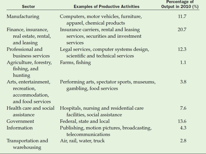
Source: Bureau of Economic Analysis, “Value Added by Industry as a Percentage of Gross Domestic Product,” December 13, 2011, www.bea.gov.
Sectors are broadly defined and include activities that, while related, are not always closely related. For example, frog farming and landscape planning are both included in the agriculture, forestry, and fishing sector.2 For this reason, other narrower types of classifications have been created.
Industry
A group of firms producing similar products or using similar processes.
Industries A very useful, and narrower, classification is to put firms into industries. An industry is a group of firms producing similar products or using similar processes. Examples of industries include aircraft, health care, soft drinks, greeting cards, and food processing. Table 12.2 gives several industries in the manufacturing sector and examples of their products. Although the firms in each of these industries are listed in the manufacturing sector, the products they produce differ significantly from industry to industry.
TABLE 12.2 Sample Industries and Products in the Manufacturing Sector
Firms producing similar products or using similar processes are grouped into the same industry.
| Industry | Industry Product Examples |
| Dairy products | Frozen custard, ice cream, juice pops, tofu frozen desserts |
| Books | Publishing and/or printing of books, pamphlets, textbooks |
| Dolls, toys, games, and sporting and athletic | Baseballs, basketballs, fishing tackle, skateboards, treadmills, playground equipment, boomerangs |
| Roasted coffee | Coffee extracts, roasting, instant coffee |
| Drugs | Antibiotics, cough remedies, lip balms, pills, poultry and animal remedies |
| Electrical industrial apparatus | Generators, motors, rotors, dynamotors, synchros |
| Carpets and rugs | Auto floor coverings, carpets, door mats, rugs, sisal floor coverings, carpet dyeing |
Source: United States Department of Labor, OSHA, www.osha.gov. Based on the Standard Industrial Classification Manual.
It is common to find large, multiproduct corporations operating in several industries. Corporate giant General Electric, for example, through its divisions and subsidiaries produces appliances, jet engines, diagnostic medical technologies, credit and loan services, railroad management technologies, and water treatment systems.3
Methods of Production
Whether a huge company such as Boeing is producing commercial jetliners or a small family-owned company is producing carpet-cleaning services, there are usually many different ways, or methods, that a business can choose to produce a good or service. The method of production actually chosen is dependent on many considerations. It is important, however, to understand that whatever that method is, it underlies the firm's cost of production.
Production Function
Shows the type and amount of output that results from a particular group of inputs when those inputs are combined in a certain way.
The Production Function A production function shows the type and amount of output that results when a particular group of inputs is processed in a certain way. Production functions exist for every good and service: tomatoes, backhoes, economics courses, rain gardens, football helmets, hamburgers, and everything else that can be produced. For most types of goods and services, such as gasoline or automobiles, production functions can be clearly defined. But we do find that for some productive activities, such as learning or child rearing, the functions are not as well understood.
A recipe, such as the one in Table 12.3, provides an easy way to understand a production function. In this production function the output is two loaves of zucchini bread. The inputs include the ingredients listed at the top of the recipe—sugar, eggs, and so forth—as well as kitchen equipment and the labor provided by the person preparing the zucchini bread. The process for combining these inputs is explained in the text of the recipe and involves such operations as grating and mixing. All production functions are similar to this recipe in that they specify a type and amount of output, the numbers and types of inputs, and how the inputs are combined.
TABLE 12.3 A Production Function
A recipe is a simple example of a production function because it gives the types and amounts of inputs and the processes needed to produce a particular output.
| Webster Groves Farmers Market Zucchini Bread |
| One of your authors has been active in the development of the local farmers market and created this zucchini bread recipe that has been used in market PR pieces. It's a really good one! |
| 3 eggs |
| 1 cup vegetable oil |
| 1 ½ cup white granulated sugar |
| ½ cup brown sugar |
| 1 T. vanilla |
| 2 cups flour |
| ½ t. salt |
| ½ t. soda |
| 2 t. baking powder |
| ½ t. cinnamon |
| 2 cups grated zucchini (Be sure to grate and not chop.) |
| ½ cup walnuts pieces |
Grease 2 loaf pans (preferably with margarine) and dust the pans with white sugar. Turn oven to 350 degrees. Grate zucchini. Beat eggs well, add oil and continue beating, add sugar and beat well. Add vanilla and beat. Add all dry ingredients and mix thoroughly; then add zucchini and nuts mixing well. Put in two loaf pans. Bake for about 45–50 minutes. Enjoy!
Usually there are several production functions to choose from when producing a good or service. For example, a painting contractor could paint the exterior of a house with brushes or spraying equipment, someone who is baking pies could make the shell from scratch or frozen dough, and a city could provide for recycling with curbside pickup or a community drop-off facility. Because a business often can choose among several methods to produce an output, it is helpful to understand the factors that underlie this choice.
Choosing a Production Function What causes a firm to choose a particular production function? This is easy to answer when we recall that the objective of a firm is to maximize profit and that profit is what remains after costs are subtracted from revenue. Every production function has a cost associated with it, and businesses will use the production method that results in the type and quality of product it wants at the lowest cost. This is not much different from the way people operate: We look for the least-cost way to accomplish something. Whether our intention is to cook a gourmet meal or a simple supper, we will try to find the production method that yields our intended result at the lowest cost. When a good or service is produced at the lowest cost, an efficient method of production and the efficient use of resources occur.
Efficient Method of Production
The lowest-cost method of production.
The choice of the production function that leads to the lowest cost for a business differs from firm to firm, even when the firms are in the same industry. Sometimes the size of an operation influences the way a business produces. Take surveillance in retail stores. It could be more cost effective for a large store to prevent shoplifting by hiring security personnel and for a small store to use cameras.
Technology
The body of knowledge that exists about production and its processes.
Production Functions and Technology Technological change has a significant influence on production functions. We can think of technology as the knowledge that we possess about production processes. Technology drives how we “do things” and it constantly changes. It affects the design of processes and machinery and equipment, and it influences inventory control, packaging, human relations, purchasing, and just about every other part of production. Technological change is leading the way to breakthroughs in the testing and treatment of medical problems, to solving crime through forensics, to advanced information systems that make e-mail and cell phones routine, and to more efficient ways to produce and distribute everything from pickup trucks to fresh herbs.
Technology defines the range of production methods from which a business can choose: from old methods to the latest advances. Even though the most technologically advanced production functions are usually the most efficient, some businesses cannot afford the transition to the latest design. Business profit may be maximized by keeping older equipment and methods. Over time, however, updated processes do become the norm.
Technology plays a major role in driving growth and change in an economy. As technology grows and new ideas are advanced, some processes and equipment become obsolete. The economist Joseph Schumpeter referred to this as creative destruction: New machinery, production processes, and other results of technological change frequently replace the old, causing one area of the economy to grow and prosper and another to shrink and perhaps ultimately disappear. For example, the introduction of robotics into assembly lines has not only affected the demand for labor but has also caused much machinery and equipment in automobile plants to become obsolete.
Creative Destruction
New, technologically advanced machinery and production methods cause the disappearance of old machinery and methods.
Creative destruction also occurs at the international level when firms in a country's industry lag because of technological advances adopted by competing firms in another country. For example, the U.S. steel and consumer electronics industries were hurt by the development of advanced production techniques for these products in Japan and elsewhere. Application 12.1, “Do You Know a Modern-Day Luddite?,” looks at the positive and negative sides of advances in technology and production that come with creative destruction.
ECONOMIC TIME, PRODUCTION, AND THE COSTS OF PRODUCTION
The production function that a firm chooses is influenced by the time frame in which it views or plans its operations. Generally, production may be regarded as taking place over a short-run or a long-run period of time. These time periods are not defined in terms of hours, months, or years (the usual custom for measuring time). Rather, they are defined in a more abstract way.
The short run is the time frame in which production takes place using some factors that can be varied in amount and some that cannot as the level of output increases or decreases. Factors of production that can be varied in amount, such as hourly labor, raw materials, and replacement parts on machinery, are variable factors. Because the amount of variable factors used changes as the level of output changes, the costs of these factors to a business also change as the level of output changes. The costs for a business's variable factors are called variable costs and include, for example, hourly wages and payments for raw materials and machine parts.
Short Run
A production time frame in which some factors of production are variable in amount and some are fixed.
Variable Factors
Factors of production that change in amount as the level of output changes.
Variable Costs
Costs of using variable factors.
APPLICATION 12.1
 DO YOU KNOW A MODERN-DAY LUDDITE?
When Joseph Schumpeter introduced the idea of creative destruction, he probably never thought that this expression would have as much relevance today as it had when he wrote in the early 1940s.
The expression itself has conflicting imagery as each word has a powerful, but different, connotation. Creative is a positive, bright, hopeful word. Destruction is a negative, dark, harmful word. And that is what creative destruction brings: positive and negative results.
On the bright side, creative destruction can be the foundation for economic growth and opportunity as new products, jobs, and advances in efficient production techniques lead to an improved quality of life and to changes that we thought were beyond our reach. Fifty years ago, the ability to talk every day to family members in other cities without spending a month's salary on long-distance phone charges was a dream. Today, the cell phone makes that dream a possibility.
On the dark side, creative destruction brings losses, sometimes profound, to businesses and employees that have a major stake in a product that is disappearing. The end of the run for many people is the fact that their products, jobs, and incomes are permanently disappearing and their lifestyles are in serious jeopardy. Think about the jobs lost with all of the online capabilities for travel, research, banking, and shopping, and the corporate losses for companies like Polaroid, Kodak, and Borders.
We sometimes use the expression “Luddite” to describe an opponent to the change that creative destruction brings. This classic expression comes from the early 19th century when the Luddites, a group of English weavers, were losing their jobs to newly designed stocking frames and power looms being introduced into clothing factories. This new technology was such a threat to the Luddites that they would storm factories in an effort to destroy the frames and looms that threatened their livelihood. Their aggression caused the passage of the Frame Breaking Act in 1812 that allowed the execution of those convicted of breaking weaving machines.
What would today's modern Luddite oppose? Certainly the Internet has brought a revolution to the way we communicate and work and the types of jobs that have been created in the past few decades. Maybe the modern Luddite experienced a job loss in the publishing or newspaper industry, or worked in a closed “record” shop that once had customers for cassette tapes and then CDs, or had a hardware store that was replaced by a big box store in a small rural town, or had a good job with a telephone company.
On the other hand, there are the employed who have benefitted from all of these changes with new jobs as computer engineers, software designers, medical technicians, and chemists and pharmacists. You might even say that the advent of cable television channels has brought professional and Olympic sports to a new level with a growth in athletes in all sorts of sports from women's basketball to curling.
Creative destruction will always be with us. It's about how we respond: Some will see the bright side and prepare themselves to move on and some will fight it.
Factors of production that cannot be changed in amount as the level of output changes are called fixed factors. Fixed factors might include a building, key personnel, some machinery, and insurance. Because the amounts of fixed factors remain unchanged as the level of production increases or decreases, their costs do not change. For example, a business might sign a lease to pay a specified rent over several years. The costs of fixed factors are called fixed costs. Importantly, fixed factors must be paid for regardless of whether the firm produces anything or not. In essence, the short run is the time period in which fixed factors form a boundary within which production takes place.
Fixed Factors
Factors of production that do not change in amount as the level of output changes.
Fixed Costs
Costs of using fixed factors.
The long run is the time frame in which all factors are regarded as variable: There are no fixed factors to limit production. In the long run, a much wider range of production choices is available because all resources, including buildings and other production facilities, are regarded as alterable.
Long Run
A production time frame in which all factors of production are variable in amount.
Suppose that the owners of a restaurant are trying to evaluate the production functions and associated costs of producing meals. If they can alter the number of servers, tables, and menu selections but not the size of the dining or kitchen area, they are planning in the short run. These same owners are planning in the long run when they analyze the methods and costs of producing meals as their facilities are expanded, or as they add new restaurants, or, more generally, when they no longer regard any of their factors as fixed.
This concept of planning in different time frames is easily applied to a student's production of a college education. The long run is the period in which general plans for earning a degree are made. In this long-run period, all factors can be altered: the selection of a college, the course of study to be followed, the number of hours to be taken each semester, and the commitment to a part-time job. Once some of these decisions are made and the student is enrolled in particular courses, producing a college education can be viewed in the short run. Each semester could represent a short-run time frame because the student is producing an education within boundaries set by the school attended, the semester's scheduled classes, and other factors to which the student is obligated.
UP FOR DEBATE
 SHOULD THE SAME COST MEASURES USED BY BUSINESSES APPLY TO GOVERNMENT AND NONPROFITS?
Issue There is a tendency to think of cost calculations as applying solely to the business sector because of the profit motive. Should all individuals and organizations seek to measure costs in the same way that businesses measure them, or are the goals of non-business entities so different that they should not focus on cost measurements in the same way?
Yes Costs are costs—they measure the value of resources used to produce “something” whether it is an SUV by an automobile company or snow plowing by a local government or a theater production by a nonprofit. All entities are well served by being data driven and reflective about how they use their scarce resources.
The basic problem of scarcity applies to all individuals and all organizations, business or otherwise. If people do not take care in calculating what costs go into a decision and take the time to evaluate those costs, they might be “missing the boat.”
Take the example of a city that provides trash collection. That city should know precisely what it costs to pick up the trash in its neighborhoods and its business districts. What is the total cost of the operation? What does it cost per household? Are costs different for residential neighborhoods than they are for business areas? Unless the city gathers and evaluates these data, it is unable to determine whether it is more efficient for the city itself to collect trash or if it is better to negotiate a contract with a private firm.
Governments and nonprofits use funds provided through taxes and contributions and other private sources. When a nonprofit has a larger than necessary administrative staff or a county government has more park rangers than it needs, resources are used inefficiently and everyone pays for this. Nonprofits and governments produce services vital to communities and the effective evaluation of costs is necessary in this service provision.
No The very basic goals of government and of nonprofits are quite different from those of a business. Businesses are created to produce profit for their owners, and governments and nonprofits exist to provide needed services for society. While it is useful to have an understanding of costs, the driving factor behind these non-business entities is different because they address societal needs.
Take the example of emergency medical services. Many communities run their own EMT or ambulance services. They do so because their citizens demand a quick response time and the best qualified technicians available in the area. The service might not be as cost effective as it could be when provided by a private company, but the residents feel more secure with their own people and equipment. Without a profit motive, a community might choose to spend more for a better service and respond to the wishes of its members.
The same might apply to many nonprofits whose function is to serve the needy or homeless in a region, or to foster the arts through theater and music, or to provide an education in a needed field. A community college, for example, might encounter very high costs to provide a nursing program, yet they do so because it fulfills a community need.
Some of the functions performed by government and nonprofits take a different, sometimes longer view, of societal needs rather than being solely profit driven. In these cases, constantly evaluating costs might not result in the best service to their communities.
In order to make production decisions in either the short run or the long run, a business needs to determine the costs associated with producing various amounts of its output. Because production is planned differently in each time frame, we will examine costs in the short run and long run separately.
Up for Debate, “Should the Same Cost Measures Used by Businesses Apply to Government and Nonprofits?,” provides an interesting issue to consider as you work through the rest of this chapter. Come back at the end of your reading of Chapter 12 and determine what your position is on this issue.
Short-Run Costs
Again, in the short run all factors used in the production of a good or service can be classified as either variable or fixed. Variable factors and costs change as the level of output changes; fixed factors and costs do not. A hypothetical example follows in which the short-run costs of operating a lawn and grounds maintenance company to service housing complexes are calculated and analyzed. The costs given in this example are those for the weekly maintenance of small apartment and condominium complex lawns and grounds.
Total Fixed Cost (TFC)
The cost of all fixed factors; does not change as the level of output changes and must be paid even when output is zero.
Total Costs Let's begin the calculation of the costs of operating this service by adding together all bills that must be paid regardless of the number of complex grounds maintained: that is, by determining total fixed costs (TFC). These could include payments on a loan for mowers and a truck as well as payments for a storage facility and insurance. Assume that total fixed costs are $400 per week.
Table 12.4, which illustrates the weekly total costs to the business of maintaining from zero through nine complexes, gives the total fixed cost for the firm's operations in the second column. Notice that the $400 fixed cost does not change as more or fewer complex grounds are maintained and that it must be paid even if none are serviced. This is because, regardless of how many lawns and grounds are cared for, the fixed factors, and thus the costs of the fixed factors, remain unchanged.
TABLE 12.4 Weekly Total Costs of Maintaining Lawns and Grounds
Total fixed cost does not change as the level of output changes and must be paid even if nothing is produced. Total variable cost is zero when nothing is produced and increases with the level of output. Because total cost is equal to total fixed plus total variable costs, it also increases as output increases.

Total Variable Cost (TVC)
The cost of all variable factors of production; increases as the level of output increases but is zero when output is zero.
Next, we will calculate the firm's total variable costs (TVC). Because these are costs of variable factors that change in amount as the number of sites maintained changes, variable costs could include expenditures for labor, gasoline, fertilizer and other chemicals, repair of the truck and mowing equipment, small hand tools, and such. The third column of Table 12.4 gives the company's total variable costs for servicing from zero through nine complexes. For example, if this firm were to service four a week, it would face a total variable cost of $350. Notice that the variable costs are zero if the firm services no grounds, they continually increase as more are maintained, and they increase significantly with a large number of complex grounds maintained. An explanation for this pattern of variable cost increases will be given shortly.
Total Cost (TC)
The cost of acquiring and using all factors of production; total fixed cost plus total variable cost.
The total cost (TC) of maintaining from zero through nine sites is given in the last column of Table 12.4. The total cost for a particular level of output is all fixed costs plus all variable costs at that level of production. For example, the total cost of maintaining five lawns and grounds is $875: $400 in fixed costs plus $475 in variable costs.
Average Total Cost (ATC)
The cost per unit of output produced; total cost divided by the number of units produced.
Unit Costs In addition to its total costs, a business usually finds it essential to determine per unit costs at each level of output. The cost per unit at a particular level of output is called average total cost (ATC). Average total cost is found by dividing total cost by the number of units produced.
TABLE 12.5 Weekly Total, Average Total, and Marginal Costs of Maintaining Lawns and Grounds
Average total cost measures the per unit cost at a specific production level, and marginal cost measures the change in total cost from producing an additional unit of output.

TABLE 12.6 Summary of Short-Run Costs
Total, average, and marginal costs are different ways of looking at costs as the level of output changes.
| Total Fixed Cost (TFC) |
|
| Total Variable Cost (TVC) |
|
| Total Cost (TC) |
|
| Average Total Cost (ATC) |
|
| Marginal Cost (MC) |
|
Table 12.5 gives the total cost of maintaining grounds from Table 12.4 and the average total cost for each individual complex when a specified number is maintained. For example, the average total cost of servicing each site when three are maintained is $225. This is found by dividing the total cost of $675 by 3. The average total cost of $185 when seven sites are maintained is found by dividing the total cost of $1,295 by 7.4
Table 12.5 also gives the marginal cost of maintaining lawns and grounds. As explained in the previous chapter, marginal cost (MC) is the change in total cost from producing one more unit of output—in this case, caring for one more site. For example, if no sites are maintained, the total cost given in Table 12.5 is $400; if one is maintained, total cost increases to $600. Thus, the marginal cost of the first complex is $200 ($600 − $400). As in the previous chapter, marginal cost is listed midway between the units of output. Table 12.6 summarizes the characteristics of short-run total, average, and marginal costs.
Marginal Cost (MC)
The change in total cost when one more unit of output is produced.
A business could analyze its unit costs in even greater detail. It could, for example, determine its fixed costs per unit (average fixed cost) and variable costs per unit (average variable cost). More detailed cost calculations such as these appear in the appendix to this chapter.
The Pattern of Short-Run Costs
There are patterns to the way total cost, average total cost, and marginal cost behave in the short run. We can observe these patterns in tables of cost figures, such as those listed in Tables 12.4 and 12.5. But they can be more easily observed when the short-run costs are graphed.
Total Cost Pattern Figure 12.1 plots the total cost, given in Table 12.5, of maintaining from zero through nine sites per week. Notice in Figure 12.1 that total cost is $400 when output is zero. This, of course, is due to the firm's fixed costs, which must be paid regardless of whether or not production occurs. Notice also that total cost continually increases as more places are serviced. Because the fixed cost of maintaining these grounds never changes, this increase is due solely to the increase in total variable costs.
FIGURE 12.1 Total Cost of Maintaining Lawns and Grounds

Total cost increases slowly when just a few sites are maintained because few variable factors are needed with the fixed factors. At higher levels of output, total cost increases quickly as more variable factors are needed to compensate for the limitations imposed by the fixed factors.
A closer analysis of total cost shows that in the early stage of production, when few sites are maintained, total cost increases slowly. But in the latter stage of production, when many sites are maintained, total cost increases quickly. Why does total cost follow this pattern?
If this company plans to service just a few places, it might manage by hiring one employee (variable factor) to use the truck and equipment (fixed factors). For each site maintained, the company would also need to provide other variable factors, such as bags for the grass clippings and gasoline for the truck and mowing equipment. However, once labor is hired, the company will not encounter significant increases in the other variable costs to care for each additional site if just a few are maintained. Thus, total cost increases slowly for the first few units of output because the increase in variable factors needed to accompany the fixed factors is small.
After a while, maintaining more sites necessitates more than just an increase in bags and gasoline. Labor costs increase as more workers are needed or as the existing employees are paid overtime. As the truck and mowing equipment are used more often, breakdowns occur, causing the cost of repairs to increase. Also, the owner of the firm may expect a higher normal profit in return for the effort and responsibility of increasing production. At some point, these increases in variable costs cause total cost to increase more quickly as production grows.
FIGURE 12.2 Marginal Cost and Average Total Cost of Maintaining Lawns and Grounds
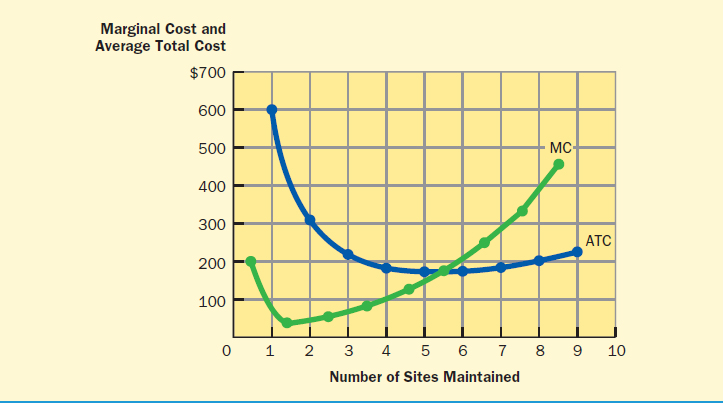
Both marginal cost and average total cost fall and then rise as production increases. When marginal cost is less than average total cost, it pulls average total cost down; when marginal cost is greater than average total cost, it pulls average total cost up.
As production increases to even higher levels, the number of places serviced will begin to seriously strain the capabilities of the fixed factors, and variable costs will increase substantially as the firm tries to compensate for the limits of the fixed factors. Perhaps, with the existing mowers and truck, the company might reasonably expect to maintain only six or seven sites. If it tries to service eight or nine, many variable factors will be needed to fill in for the limitations of the fixed factors. At this point, the company may encounter considerably higher variable costs as it rents another truck and more mowers, leases additional storage space, and hires a manager.
In short, total cost increases slowly at first because, with a given amount of fixed factors, few variable factors can increase production significantly. As output levels become larger, total cost increases more rapidly because more variable factors are needed with the fixed factors to increase production. At high levels of production, costs increase very quickly because the fixed factors are approaching the limits of their productivity, and many variable factors are needed to compensate for the fixed factor boundary.
Marginal Cost and Average Total Cost Patterns Let us next examine the marginal cost (MC) and average total cost (ATC) patterns as production increases. The marginal cost and average total cost data given in Table 12.5 are graphed in Figure 12.2.
Notice that marginal cost, or the change in total cost from maintaining one more site, decreases at first and then increases. As with total cost, this drop and rise are due to the behavior of the variable factors as reflected in variable costs. With this in mind, the same reasoning that applies to the explanation of the total cost pattern applies to the explanation of the marginal cost pattern.
To service the first site, the marginal cost is $200. If you refer to Table 12.4, you can confirm that this equals the change in variable cost (and total cost) associated with maintaining one rather than no sites. Much of this $200 marginal cost is probably due to the hiring of labor. To maintain a second site, the marginal cost is only $25. This decrease in marginal cost occurs because the additional variable factors needed to maintain the second site cost the firm only $25. As explained earlier, at this point there will be only a slight increase in the use of some variable inputs, such as gasoline and grass bags.
When a third site is maintained, marginal cost begins to rise because of the increase in variable factors needed to increase production. And as more and more places are cared for, marginal cost rises more rapidly. This more rapid rise is due to the increasing amounts of variable factors that are required to compensate for the limits placed on production by the fixed factors.
Return to Figure 12.2 and observe the average total cost curve. Average total cost decreases and then increases with more production. Why is this so?
The cost per unit falls initially because marginal cost is lower than average total cost. When marginal cost is less than average total cost, it pulls average total cost down. When marginal cost becomes greater than average total cost, it pulls average total cost up. Figure 12.2 also shows that because of these relationships between average and marginal costs, marginal cost must cross, or equal, average total cost at minimum average total cost. Thus, average total cost behaves the way it does because of the behavior of marginal cost.
You encounter this relationship between marginal and average values in determining your average in a course as you take additional exams. If you make a grade on your next exam (remember: each additional exam that you take is a marginal exam) that is lower than your average, that grade will pull your average down. If, on the next exam, you make a grade higher than your average, your average will increase. For example, if you have an average of 93 percent in this economics course and you earn a grade of 70 percent on your next exam, your average will fall; if you earn a grade of 98 percent on your next exam, your average will rise. Test Your Understanding, “Calculating Costs and Averages,” gives you an opportunity to further explore the average–marginal relationship and to calculate some short-run costs.
The Law of Diminishing Returns
Law of Diminishing Returns
As additional units of a variable factor are added to a fixed factor, beyond some point the additional product from each additional unit of the variable factor decreases.
Underlying all the short-run cost patterns is a basic principle, which you may likely have heard, called the Law of Diminishing Returns. This law states that as additional units of a variable factor are added to a fixed factor, beyond some point (not necessarily right away) the additional product from each additional unit of the variable factor decreases. Put another way, the Law of Diminishing Returns says that, after some point, each additional unit of a variable factor used will add less to output than was added by the unit used just before it. This is easily illustrated with an example.
Assume that you own a small restaurant and plan to begin hiring people to prepare and serve meals. The dining room, outfitted with tables and other restaurant furniture, and a fully equipped kitchen are the fixed factors, and the labor used to work in the restaurant is a variable factor.
If one person is hired to work in the restaurant, that person working alone will need to prepare, serve, and clean up after a certain number of meals per day. If a second person is hired, the two together can divide up some of the tasks and work more efficiently. One person can work the kitchen and the other can work the dining room. Together the two will more than double the number of meals that can be prepared and served by one person alone. If you hire a third person, work can be further divided, and the number of meals may again significantly increase. As long as each worker hired adds more to output than was added by the worker hired just before, or as long as diminishing returns don't set in, the marginal cost of each additional meal falls.
TEST YOUR UNDERSTANDING
 CALCULATING COSTS AND AVERAGES
- A student's grade in a psychology class at a state university is determined by averaging the percentage scores of four equally weighted exams. One of the students in the class earns a grade of 92 percent on the first exam, 79 percent on the second, 80 percent on the third, and 93 percent on the fourth.
The student's average after the first exam is ____ percent. After the second exam, the student's average will ____ (rise or fall) because the marginal score from the second exam is ____ (higher or lower) than the average after the first exam. After two exams, the student's average is ____ percent.
The student's average after the third exam will ____ (rise or fall) because the marginal score from the third exam is ____ (higher or lower) than the average. After three exams, the student's average is ____ percent.
The student's average after the fourth exam will ____ (rise or fall) because the marginal score from the fourth exam is (higher or lower) than the average. After four exams, the student's average for the course is ____ percent.
- Bert's Trash Company specializes in emptying large commercial recycling containers and delivering the material to a regional single-stream sorting facility. Bert has figured that his total fixed costs per business day are $100. He has also calculated that the total variable cost for one pickup is $250 per day, the total cost for three pickups per day is $400, the marginal cost of the second pickup as well as the fourth pickup is $50, and the average total cost with five pickups is $105. Fill in the following table for Bert's costs.

- The manager of a college food service has determined that the daily fixed cost of operation is $855. She has also calculated that the total variable cost for preparing 900 meals is $1,170; for preparing 1,800 meals, it is $2,565; and when 2,700 meals are prepared, total variable cost equals $5,328.
Given this information,
the total cost for 900 meals is $ ____,
the total cost for 1,800 meals is $ ____,
the total cost for 2,700 meals is $ ____,
the ATC per meal with 900 meals is $ ____,
the ATC per meal with 1,800 meals is $ ____, and
the ATC per meal with 2,700 meals is $ ____.
- Assume that the following table applies to the costs of completing the short-form federal income tax return for students by a small accounting service. Fill in this table.

Answers can be found at the back of the book.
At some point, assume when the fourth person is hired, the number of meals that can be prepared and served per day will no longer increase as rapidly with additional workers. That is, the number of additional meals prepared and served by hiring the fourth worker will not be as great as the number of additional meals prepared and served by hiring the third worker. Four workers cannot operate as efficiently as three because the fixed facility is becoming crowded. In other words, the boundary imposed by the fixed factors begins to limit the productivity of the variable factor. When this occurs, and the additional output from hiring an additional worker begins to fall, diminishing returns have set in. This causes the marginal cost of each additional meal to rise.
Beyond this point, as more (five, six, seven) people are hired, the additional work accomplished by each will further diminish. They will become less efficient as the fixed factors more severely limit their full use, and marginal cost will rise at a faster rate. It would, incidentally, be possible to hire so many restaurant workers that they would get in each other's way, causing output to fall.5
The Law of Diminishing Returns governs all production in the short run. For example, when a student tries to produce enough knowledge to pass an exam by studying for an extended and uninterrupted period of time, the Law of Diminishing Returns takes effect. During the first few hours of reading and reviewing, each hour will produce more additional knowledge than the hour before it as the material is comprehended. After a while, however, as the student becomes tired and fixed physical and mental factors approach their limit, diminishing returns take effect, and each additional hour of study is less productive than the one before it. Can you use the Law of Diminishing Returns to explain why it is better to study on a consistent basis for shorter periods of time than it is to cram the night before an exam?
While the Law of Diminishing Returns and the resulting pattern of costs given here are common to all production in the short run, the point at which diminishing returns set in differs from product to product. But these differences do not undermine the fact that all short-run production can be explained in terms of these patterns: The limitation of the fixed factors, which gives the short run its definition, causes diminishing returns to occur and thus causes marginal, average total, and total costs to rise in the latter stages of production.
Businesses are always trying to find ways to lower their costs, often by making their inputs more productive. Application 12.2, “Are Wellness Programs Cost Effective?,” discusses the argument that employer-provided opportunities to create a healthier lifestyle for employees helps to reduce costs. If wellness programs work, how could they influence the Law of Diminishing Returns?
Long-Run Costs
The long run is the time frame long enough for a business to regard all its factors of production as variable and none as fixed. Calculating the cost of production in the long run means determining the cost of a given level of output when a business can alter the amounts of any and all of its resources. In the long run, production costs are not divided between fixed and variable because all factors, and therefore all costs, are variable.
Table 12.7 gives the long-run costs of constructing from zero through 10 houses by a hypothetical home builder. The second column of Table 12.7 gives the long-run total cost of constructing these houses. Notice that long-run total cost increases as more houses are produced and that, because there are no fixed factors or costs, it is zero when no houses are produced.
Long-Run Total Cost, Average Total Cost, and Marginal Cost
Total cost, per unit cost, and cost per additional unit of output, respectively; calculated for production when all inputs are regarded as variable.
APPLICATION 12.2
ARE WELLNESS PROGRAMS COST EFFECTIVE?
Many organizations provide wellness programs for their employees. These range from fitness centers and weight-loss programs and contests to flu shots. While the purpose of these programs is to help employees live longer, healthier lives, there seem to be cost-reduction benefits for an organization that pursues them.
There are costs for providing wellness programs: expenditures to develop them, staff time to administer them, and lost work hours for employees who participate. But, these costs must be balanced against the benefits that can be realized from staffing with a healthier workforce.
Healthier employees have lower absentee rates resulting in less overtime for other employees who need to cover for someone who is absent or for the loss of service that can occur. There is positive evidence of this in all types of organizations from restaurants to fire departments to banks.
Healthier employees reduce costly turnover in an organization. Turnovers mean more staff time devoted to hiring and increased expenditures for training. In many job situations turnover is expensive. Consider the costs to do a search for and hire a new college president, a corporate CEO, or a university faculty member. Training costs are high for new police officers and fire fighters.
One of the most important benefits to wellness programs is the reduced cost in health and life insurance premiums that an organization can experience. Today, employers wrestle with the cost of providing health care benefits which in many cases add thousands of dollars a year to the cost of each employee. When fewer health care claims are made, premiums tend to be lower.
Not everyone agrees that it is the obligation of an employer to provide wellness programs and opportunities, and some do not believe that it lowers costs. There are those who think that the decisions involved in leading a healthier life—getting flu shots, exercising, not smoking—are made by individuals who will invest their efforts and personal funds in pursuing wellness regardless of whether an employer provides them or not. People on this side of the argument might even think that an employer is unnecessarily raising its costs by providing wellness opportunities. They believe that health is a lifestyle choice regardless of where a person works.
As debates about wellness programs continue, it is interesting to look around at college campuses and community recreation centers. These centers have become almost as important as a library and, in many cases, have far more visitors than the library. This may be making a statement about how much we value exercise and physical activity. Does this focus on campus and community fitness replace the need for employers to provide wellness programs or does it make their provision more important?
Long-run total cost is used to calculate long-run average total cost, which is determined in the same way as short-run average total cost: Total cost is divided by the quantity of output produced. Long-run average total cost is shown in the third column of Table 12.7. Long-run marginal cost can also be calculated from long-run total cost: It is the change in long-run total cost as one more unit of output is produced.
Economists like to focus on the pattern of long-run average total cost when analyzing the behavior of production and its costs in the long run. Figure 12.3 plots the long-run average total cost from Table 12.7. Notice that, at first, long-run average total cost decreases as the level of output increases. With an ability to vary inputs that were fixed in the short run, the company finds that, initially, the cost per unit of output drops. At some point long-run average total cost reaches a minimum and, in this example, stays at that level for a while as output continues to grow. But at some point, as production increases even further, the cost per unit of output increases. The explanation for this decreasing, constant, and increasing cost pattern, which is typical of the behavior of long-run average total cost, is based on economies of scale, constant returns to scale, and diseconomies of scale.
Economies of Scale
Occur when the increasing size of production in the long run causes the per unit cost of production to fall.
Economies of Scale, Diseconomies of Scale, and Constant Returns to Scale In the initial stages of long-run production a producer typically experiences economies of scale that cause long-run average total cost to decrease. This means that initially as the size, or scale, of the operation becomes larger, the cost per unit of output falls. What causes economies of scale to occur?
TABLE 12.7 Long-Run Total Cost, Average Total Cost, and Marginal Cost
Long-run total cost is the total expenditure for each level of output in the long run. Long-run average total cost measures the per unit cost; and long-run marginal cost measures the cost of producing an additional unit of output.

With a larger scale and output, a firm can use highly specialized and efficient labor and equipment that might be expensive to obtain, but because of the large output, can actually allow the firm to produce at a lower per unit cost. Economies of scale permit a company to hire more specialized professionals who can apply their expertise to specific areas of the company's operations, such as human resources or finance or supply-chain management. A large company can profitably use more advanced technology and equipment, from bucket trucks to accounting and software systems. Also, as a business becomes large, it may receive quantity discounts on some of its purchases, as well as negotiate lower interest rates on its loans. Think about fast-food restaurants and your local pub. The cost per unit of a burger that is carefully machine-sized, prepackaged, and frozen for instant grilling by an unskilled worker is considerably less than one made by a cook who is starting with fresh ingredients from a local market.
Unit cost savings, or efficiency gains, from economies of scale as a business becomes larger and produces higher levels of output have been a frequent argument in favor of allowing mergers between competing sellers in the same market. Mergers are covered in more detail in Chapter 14.
FIGURE 12.3 Long-Run Average Total Cost

A typical long-run average total cost curve follows a pattern of decreasing, constant, and increasing per unit costs.
When cost per unit increases in the latter stages of long-run production, a firm experiences diseconomies of scale. In this case, the size or scale of the operation has become so large and unwieldy that the cost per unit of output increases. Diseconomies of scale generally arise because the large size of a company makes control over its operations difficult. As the organization grows and the chain of command lengthens and becomes more complex, it is necessary to hire more managers at all levels, thereby increasing the cost of output. With a longer chain of command, authority and responsibility may become disjointed, causing factors of production to be wasted due to a lack of communication, accountability, or poor control. Costs may also be affected by the amount of time required to pass information and commands through such a large organization. Many companies have restructured or reorganized in an effort to reduce diseconomies of scale created by layers of management.
Diseconomies of Scale
Occur when the increasing size of production in the long run causes the per unit cost of production to rise.
Between economies of scale and diseconomies of scale is a range of production where long-run average total cost neither decreases nor increases. Throughout this output range the firm experiences constant returns to scale, or operating levels that have become so large that economies of scale are exhausted but not large enough to encounter diseconomies of scale.
Constant Returns to Scale
Occur in the range of production levels in which long-run average total cost is constant.
Many real-life examples attest to the existence of economies and diseconomies of scale. This does not mean, however, that every company faces a long-run average total cost curve that looks exactly like that in Figure 12.3. Instead, the long-run average total cost of each firm's product differs in the length and strength of its decreasing, constant, and increasing ranges. A company producing automobiles, for example, will have a different length and strength to its long-run average total cost curve phases than will a fast-food chain producing hamburgers. Figure 12.4 gives the three phases of long-run production costs.
Application 12.3, “A Distance-Ed Student Puts His Lessons to Work on a Farm,” provides a real-life application of many of the concepts and terms that you have learned in this chapter. As you read about Jeremy, think about technology and production functions, fixed and variable costs, the short run and long run, and economies of scale.
FIGURE 12.4 The Three Phases of the Long-Run Average Total Cost Curve

The long-run average total cost curve goes through three phases: a decreasing per unit cost phase caused by economies of scale; a phase of constant returns to scale where per unit costs neither decrease nor increase; and a phase where per unit costs increase due to diseconomies of scale.
APPLICATION 12.3
A DISTANCE-ED STUDENT PUTS HIS LESSONS TO WORK ON A FARM
A huge great dane named Dottie barks a greeting as Jeremy Groeteke parks his Dodge Durango [after driving two hours from the University of Nebraska where he is earning a master's degree in plant physiology] before the large brick farmhouse where he grew up. In Lincoln . . . he goes to class and finds a few hours to take a separate distance-education course on an advanced farming technique called precision agriculture. On weekends he drives back here to help raise corn and soybeans on the family farm.
This part of Boone County doesn't have cable television, a 911 system, or a shopping mall. But the Groeteke farm uses state-of-the-art technology—including Global Positioning System satellites, computer databases, and wireless networks. And Jeremy, who at 24 is the youngest of the family's three sons, is the one pushing to make the farm high-tech.
The precision-agriculture techniques he is learning through the university's distance-education program use computers to compile detailed information about each field. The computers, installed in tractors and lined to G.P.S. satellites, can control modern seed- and fertilizer-spreading equipment and, later, weigh crops as they're harvested, telling the farmer exactly how much seed produced how much corn in a given location.
With yield information detailed down to every three or four feet, farmers can then customize the treatment of their fields to increase production further, applying water, seed, and fertilizer in precise amounts.
Over homemade peach pie, Jeremy's father says precision agriculture should help the farm make more money with less work. He doesn't believe investing in technology is a big gamble. “We take a lot bigger risks with a lot of other things—the market, the weather,”. . . . “And those are things we really can't control.”
Precision agriculture is important to the Groetekes because acreage they farm—their own and fields they rent from others has grown. . . . The larger the farm gets, the more helpful precision agriculture becomes. . . .
Source: Copyright 2001, The Chronicle of Higher Education. Reprinted with permission.
Summary
- The greatest portion of measured output in the U.S. economy comes through the business sector. Categories have been developed for classifying production. Producing sectors is a broad category that includes the services, manufacturing, and other sectors; industry is a narrower category that includes firms producing similar products or using similar processes.
- A production function shows the output that results when a particular group of inputs is processed in a certain way. Firms have a choice of production functions and seek the least-cost, or efficient, method for producing a desired quantity and quality of output in order to maximize profit.
- The development of new productive inputs and techniques can come from technological change. Technological change can also lead to creative destruction: New inputs and processes cause those currently in use to become obsolete and some areas of an economy to grow while others decline.
- The choice of a method of production is influenced by the time frame in which a business plans its operations. The short run is a time period in which some factors of production are variable in amount and some are fixed. The capabilities of the fixed factors, because they cannot be changed, serve as a boundary within which production takes place. The long run is a time period in which all factors are regarded as variable.
- In the short run, the total cost of producing a certain level of output is found by adding total fixed cost and total variable cost. Total fixed cost is the same regardless of how much is produced; total variable cost increases as output increases. Average total cost is the cost per unit of output at a given level of production and is found by dividing total cost by the number of units of output produced. Marginal cost is the change in total cost resulting from the production of an additional unit of output.
- In the short run, total cost increases slowly at low levels of output and rapidly at high levels of output. Average total cost decreases and then increases, as does marginal cost. These patterns are the result of the way in which variable factor usage increases as production increases. At low levels of output, small amounts of variable factors are needed with the fixed factors, and at high levels of output, large amounts of variable factors are needed to compensate for the limits imposed by the fixed factors.
- Underlying the patterns of short-run costs is the Law of Diminishing Returns, which says that as a variable factor of production is added to fixed factors, beyond some point the additional product from each additional unit of the variable factor will decrease.
- Long-run average total cost illustrates the pattern of costs in the long run. The shape of the long-run average total cost curve is the result of economies of scale that occur in the early stages of long-run production and cause the cost per unit of output to drop, constant returns to scale where average total cost stays the same, and diseconomies of scale that occur in the late stages of long-run production and cause the cost per unit of output to increase.
Key Terms and Concepts
Producing sectors
Industry
Production function
Efficient method of production
Technology
Creative destruction
Short run
Variable factors
Variable costs
Fixed factors
Fixed costs
Long run
Total fixed cost (TFC)
Total variable cost (TVC)
Total cost (TC)
Average total cost (ATC)
Marginal cost (MC)
Law of Diminishing Returns
Long-run total cost, average total cost, and marginal cost
Economies of scale
Diseconomies of scale
Constant returns to scale
Review Questions
- What is a producing sector? Give some examples. How does this differ from the industry classification?
- A friend believes that, as far as the costs of operating a business are concerned, short-run costs are the costs that are incurred within the current year and long-run costs are those spread over more than a year. As a student of economics, how would you explain these costs differently to your friend?
- The short-run average total cost curve and the long-run average total cost curve are similarly shaped. What causes the short-run average total cost curve to slope down and then up? What causes the long-run average total cost curve to slope down and then up?
- When marginal cost is less than average total cost, average total cost decreases. When marginal cost is greater than average total cost, average total cost increases. Why is this so?
- Why does a firm incur fixed costs over the short run when its output is zero, and why do fixed costs not change as the level of output changes? Why does a firm's short-run total variable cost increase slowly at smaller levels of output and rapidly at larger levels of output?
- What is the Law of Diminishing Returns and why does it affect short-run but not long-run production? How will the Law of Diminishing Returns affect the productivity of each additional student who is washing cars at a local church parking lot to raise money for a charity? Why does this effect occur?
- Complete the following table of short-run costs. From the information in the completed table, plot a total cost curve on the left-hand graph that follows the table and an average total cost curve and a marginal cost curve on the right-hand graph. Remember to plot marginal cost at the midpoint.

- Identify the three phases of a long-run average total cost curve. What is the reason for the behavior of long-run average total cost in each phase?
Review Questions
- Can you construct a production function for earning an A in this course?
- What are the necessary inputs?
- How much of each input is required?
- How are the inputs combined?
Does the production function for producing an A in a course differ by course?
- List some possible explanations for the differences in production techniques used by two pizza restaurants: One is an independent mom-and-pop operation and the other is part of a national chain.
- Technological change can cause creative destruction: Because of new technology, one area of an economy expands while another contracts and perhaps disappears. Give some recent examples of the process of creative destruction on the national level and on the international level. What products, industries, and jobs were affected in each of your examples?
- The Law of Diminishing Returns was introduced in this chapter and the Law of Diminishing Marginal Utility was introduced in Chapter 11. Are there any similarities between a business using additional units of a variable input to produce a good in the short run in order to maximize profit and an individual consuming additional units of a good in order to maximize utility?
- Indicate whether each of the following is probably a fixed factor or a variable factor in the short run.
- Raw materials going into a production process
- The heat required to keep the pipes in a warehouse from freezing
- Electricity used to run machinery and equipment
- The only person in a company who knows the trade secret formula to a highly profitable product
- A desktop computer
- A companywide computer-based software accounting system
- Suppose a proposal is offered to consolidate the more than 75 towns surrounding a large city into a few larger towns. What economies of scale affecting fire, police, administrative, and other services might result from the consolidation? What diseconomies of scale might result from the creation of a few large towns in place of many small ones? From an economic point of view, would you favor this proposal? Why?
- How might a business's ability to take advantage of economies of scale affect the price it charges for its product, its profitability, and its competitiveness with rival sellers? What concerns could diseconomies of scale create for pricing, profitability, and competitiveness?
- We have all been in situations where we see or experience employees standing around and chatting and seemingly not working at their jobs. Discuss an example you have encountered. Do you believe this was due to diseconomies of scale?
Critical Thinking Case 12 
THE HUMAN FACTOR
Critical Thinking Skills
Appreciation for a broad perspective
Understanding behavioral considerations
Economic Concepts
The Law of Diminishing Returns
Short- and long-run costs
Creative destruction
Too often, there is a sterile, robotic view of factors of production, their costs, and cost-cutting for a business. Workers and managers, while recognized for the important roles they play, can be regarded like machines or buildings or any other resource needed to produce a good or service. But people are complex creatures with personal objectives, needs, and feelings. To neglect this personal side of employees is not smart: It can lead to underutilization of employees, stand in the way of solving problems, and ultimately affect costs.
In a perfect world, a manager would staff an operation with the “right” number of employees; that is, the number that would keep costs down. But a manager could have other objectives, like “empire building.” That is, a manager could think that having a large staff moves one up in the ranks and increases power, visibility, and influence. This type of manager might want to increase the size of an operating area for “career” reasons that could be costly to the business.
Or an organization that is struggling with its costs might need to lay off a few employees. In working through a reduction in force, a company could simply let those with the least seniority go—an easy way to address an often-difficult process. But there may be employees with good potential to improve production and increase the profitability of the organization in the future among this group. Again, a sterile view of workers does not recognize the unique abilities of employees who are valuable contributors to an employer.
The human factor is also related to the communication that occurs within an organization. With growth in the ability to rapidly communicate through methods such as text messaging and e-mail, it is easy to be in touch with virtually everyone in an organization and beyond. But how does a person decide what is necessary communication to do an effective job and what is extraneous, time consuming, and unnecessary? Answering those 200 e-mail messages a day takes time away from real production and raises costs.
We might also consider the sense of interconnectedness with one another that seems to be disappearing as, more and more, employees communicate electronically and spend less time meeting face-to-face. Today's workplace puts less emphasis on conversation and collegiality and more on sitting alone behind a desk and looking at a screen. This can lead to an increased sense of isolation and loss of commitment to an organization, which may lead to higher costs.
Questions
- In addition to empire building and self-promotion, what other managerial traits have you seen that may not necessarily reduce costs?
- How do today's communication systems lead to cost savings? How do they lead to increased costs? In your opinion, do the savings outweigh the losses?
- How would you go about measuring whether the decreasing interconnectedness among people at work raises or lowers costs? Are there any strategies to improve this situation?
CHAPTER 12 APPENDIX
A FURTHER LOOK AT SHORT-RUN AVERAGE AND MARGINAL COSTS
A business may want to know more about its per unit costs than can be learned from a calculation of average total cost alone. Just as total cost is made up of total fixed and total variable costs, average total cost is made up of average fixed and average variable costs. A knowledge of how average fixed and average variable costs change as the level of output changes, and how these changes affect average total cost, is useful to a business when making production, pricing, and other decisions that impact its profitability.
Calculating Average Fixed and Average Variable Costs
We have already learned that average total cost is total cost per unit of output and that it is found by dividing total cost by the number of units produced. Similarly, average fixed cost (AFC) and average variable cost (AVC) are the fixed and variable costs per unit of output, and are calculated by dividing total fixed cost and total variable cost, respectively, by the number of units produced.
TABLE 12A.1 Weekly Total, Average, and Marginal Costs of Maintaining Lawns and Grounds
Average variable cost and average total cost behave as they do because of the behavior of marginal cost. Marginal cost behaves as it does because of the Law of Diminishing Returns.

FIGURE 12A.1 Marginal and Average Costs of Maintaining Lawns and Grounds

Average variable cost and average total cost behave as they do because of the behavior of marginal cost. Marginal cost behaves as it does because of the Law of Diminishing Returns.
Table 12A.1 shows the weekly total fixed cost, total variable cost, and total cost numbers from Table 12.4, as well as the average total cost and marginal cost numbers from Table 12.5, for maintaining different numbers of housing complex grounds. Table 12A.1 also gives the average fixed and average variable costs that are calculated from those numbers.
It is easy to see in Table 12A.1 how the different average costs are calculated. For example, for five sites the average fixed cost of $80 is found by dividing the total fixed cost of $400 by 5; the average variable cost of $95 is the $475 total variable cost divided by 5; and the average total cost of $175 is the total cost of $875 divided by 5. The average total cost of $175 can also be found by adding the average fixed cost of $80 to the average variable cost of $95.
Notice in Table 12A.1 how average fixed and average variable costs change as more sites are maintained. Since total fixed cost does not change as the level of output increases, the average fixed cost assignable to each unit produced (in this case, each site maintained) gets smaller and smaller as more is produced. This is sometimes referred to as “spreading the overhead.” Average variable cost, on the other hand, decreases at first and then increases at larger levels of output. The explanation for this is the same as the explanation for the behavior of average total cost and is more clearly understood when looking at a graph of average variable cost and marginal cost.
Graphing Average and Marginal Cost Curves
The average total, average variable, and marginal cost information from Table 12A.1 is graphed in Figure 12A.1. Two of the curves in the figure, average total cost (ATC) and marginal cost (MC), are identical to the average total and marginal cost curves in Figure 12.2.
FIGURE 12A.2 Average Fixed, Variable, and Total Costs of Maintaining Lawns and Grounds
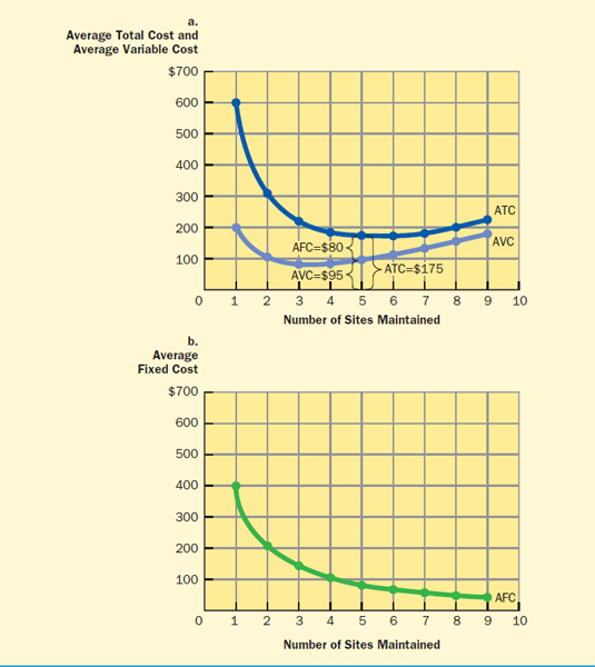
Average fixed cost is shown by the difference between the ATC and the AVC curves. The curves come closer together as the level of output increases because average fixed cost decreases.
Notice again that the ATC curve falls when marginal cost is below average total cost, the ATC curve rises when marginal cost is above average total cost, and the ATC curve is at its lowest point when it is equal to marginal cost. Figure 12A.1 also shows exactly this same relationship between marginal cost and average variable cost. Depending on whether it is below, equal to, or above average variable cost, marginal cost pulls the AVC curve down, sets its minimum value, or pulls it up. As was the case with average total cost, this behavior of average variable cost is explained by the mathematical relationship between average and marginal measurements.
The basic economic reality underlying these relationships is, as indicated in the chapter, the Law of Diminishing Returns. Initially, as additional units of a variable factor are employed along with a fixed factor, the fixed factor is utilized more efficiently and marginal cost falls. At larger levels of output, after diminishing returns set in and the limitations of the fixed factor begin to be felt, each additional unit of the variable factor adds less to output than did the previous unit, and marginal cost begins to rise. At very high levels of output, where many additional units of the variable factor are needed to compensate for the now-serious limitations of the fixed factor, marginal cost rises more rapidly. Thus, the Law of Diminishing Returns, which affects how variable and fixed factors interact with one another, causes marginal cost to behave as it does, and the behavior of marginal cost causes average variable and average total costs to behave as they do.
Average Fixed Cost Average fixed cost is the difference between average total cost and average variable cost; it is shown in Figure 12A.2a by the distance between the ATC and AVC curves. For example, at one site maintained, the ATC curve indicates that average total cost is $600 and the AVC curve indicates that average variable cost is $200. The difference between the two curves is $400, which, as Table 12A.1 shows, is the average fixed cost for maintaining one site. At five sites the ATC curve is at $175 and the AVC curve is at $95. The difference, $80, is equal to average fixed cost at five complexes.
Figure 12A.2a highlights the costs at five sites maintained to strengthen your understanding of how average variable and average fixed costs equal average total cost. Also, it should be clear by now why the distance between the ATC and the AVC curves decreases as the level of output increases: Average fixed cost is decreasing. Decreasing average fixed cost is illustrated in Figure 12A.2b.
1 Economic Report of the President (Washington, DC: U.S. Government Printing Office, 2012), Table B–1.
2 Executive Office of the President, Office of Management and Budget, Standard Industrial Classification Manual, 1987 (Washington, DC: U.S. Government Printing Office), pp. 29, 34.
3 http://www.ge.com, 3/10/2012.
4 The average total cost of maintaining zero lawns is not given because any number divided by zero is undefined.
5 This means that a point can be reached where more would be produced if some of the workers would quit.