
Chapter Seventeen
Data
Every sports rating model in this book requires that data on certain game statistics be used as input to the model. Thanks to the Web, finding this data is not hard. However, entering it into a format that is friendly to computer algorithms is. At the heart of each rating model presented here is a matrix which, once built, is then analyzed. Even for tiny examples building this matrix by manual data entry quickly becomes tedious. Thus, one must either (a) create a tool such as a perl-scripted web scraper that automatically converts the data available on webpages into an algorithm-friendly format or (b) find the data already in such a format. Of course, most of us, given the choice, would opt for (b). Thanks to Ken Massey, of the Massey model of Chapter 2, we can. Just what a luxury this is becomes apparent when we apply these rating models to other non-sports contexts such as politics, entertainment, or science.
Massey’s Sports Data Server
Ken Massey of the Massey model (Chapter 2) has created a wonderful resource for obtaining sports-related data. His website, www.masseyratings.com, contains an enormous amount of information. In particular, the data webpage at www.masseyratings.com/data.php can be used to build the models presented in this book. At the bottom of this page, you can find links to data for a range of sports, categorized according to levels and seasons within each sport. For instance, Massey currently has data for baseball, basketball, football, hockey, and lacrosse and it seems he has plans to add data for additional sports soon. Most sports are further subdivided. For instance, the hockey category contains data for the National Hockey League, the college men’s league, and the college women’s league. Some categories have data for several seasons. For instance, Major League Baseball has data for each season since 1990.
Figure 17.1 shows a screen shot of data served up by Massey’s tool for a request on NCAA men’s Division 1 college basketball games for the 2007 season. We have attached text labels to the figure to identify the data represented in each column. Of course, the data server always serves up data in the same format, which is ideal for writing programs. Another great feature of Massey’s data server is the number of options for “subsetting” the data. For instance, for a men’s college basketball request one can choose from NCCAA, NJCAA, both NAIA divisions, and all three NCAA divisions (or get the combined data for absolutely every college basketball game that year). Or the data can be requested for a particular conference such as the NCAA’s Division 1 Northeast Conference. Or the data can be requested for all inter-conference games for all of Division 1. Or . . . you get the idea. Ken Massey has tried to accommodate nearly every conceivable data request, as the number of options for navigating through the system is staggering. Massey’s server was our portal to the data used for every sports ranking example in this book.
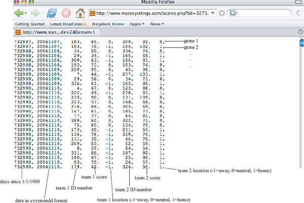
Figure 17.1 Screen shot of Massey’s sports data server
Pomeroy’s College Basketball Data
If college basketball is your sport, then Ken Pomeroy is your source. He produces ratings for college basketball teams and his website contains a wealth of data pertaining to specific statistics such as offensive and defensive rebounds, free throw, two point and three point shooting percentage, and turnovers. Pomeroy has posted this data in comma-separated files that are available for download from his website, www.kempom.com.
Scraping Your Own Data
While Massey’s data server can answer a multitude of sports data needs, there are some it cannot answer. For instance, some advanced variants of the OD and Markov models request sports data beyond simple point scores. To construct a Markov model with, say, rebounds, unfortunately you will need to turn to a source other than Massey’s server. At first, you might stubbornly hang onto the futile hope of finding a similar server for these additional statistics. After giving up the dream of a perfect server for all your data needs, you then assess the importance of the added statistic(s). If you deem the additional data essential to the model, then you must collect it yourself. And this is the art of scraping your own data—the act of writing a script that locates the precise piece of data you want on a particular webpage and scrapes that data into a text file in a format of your choosing. Typically you will need your tool to periodically scrape the list of chosen webpages, for instance, weekly if you are collecting football data as the season progresses. Of course, all this assumes that you have identified these scrape-able webpages, which requires considerable time on your part. Nevertheless, scraping your data provides you with the most freedom and flexibility. The possibilities truly are endless to a skilled scraper, which is to say this is a valuable programming skill worth acquiring (which is to say we wish we would have acquired it along the way).
Now if you missed the lesson on data scraping during your school days, our advice is to find a student who didn’t. We were each lucky enough to have mathematics students with programming skills. N.C. State University student Anjela Govan wrote her own perl scripts to scrape data on NFL games as part of her doctoral dissertation [34]. And Ryan Parker of the College of Charleston is a pro data scraper—quite literally, see the aside on p. 219. He is an NBA fan and fanatic. He has written programs to scrape data from sites such as ESPN.com and NBA.com on a nightly basis. Ryan has every conceivable statistic. To give you an idea of just how massive his data repository is, Ryan could identify which ten players were on the court on the eleventh game of the season during the twelfth minute of play. This level of detail is important for Ryan’s research, which concerns predicting outcomes (0, 1, 2, 3, 4, or 5 points) on a possession by possession basis. See his blog www.basketballgeek.com for more on his research and data. In summary, if you need NFL data, contact Anjela Govan. If you need NBA data, Ryan’s your man.
ASIDE: Team Geek
In recent decades, the staff for professional sports teams has grown dramatically. First, the coaching staff grew. Teams now have a head coach, assistant coach, second, third, fourth, etc. assistant coaches, offensive specialists, defensive specialists, shooting coaches, and so on. Now teams travel with even bigger entourages, including the team trainer, dietician, and massage therapist. It’s the latest addition of the staff that most excites us. It seems the latest trend in the NBA is to hire a “team geek.” This new staff member studies mathematical and statistical data to identify any trends or historical tendencies that might be useful to the team. Several NBA teams have contacted the College of Charleston senior Ryan Parker. Ryan hosts his own website, www.basketballgeek.com, where he collects copious amounts of NBA data. Ask Ryan for any statistic on any player on any team, and he’ll email back with the precise needle in the haystack that you need. Ryan analyzes this data to uncover information that might be useful to coaches. For instance, as part of his senior thesis, Ryan analyzed team possessions and tried to find which combinations of players are most likely to score 3 points or 4 points in the final possession of a game. This is important information for coaches in the waning seconds of a game. While it hasn’t happened yet, here’s the scenario we one day envision for Ryan and his fellow team geeks. There are eight seconds left in the game, with his team down by three points, the five opposing players on the court and his guard about to inbound the ball at mid-court, the coach takes a timeout and turns to Ryan and asks, “According to your statistical and mathematical analysis, what’s our optimal strategy?”
Creating Pair-wise Comparison Matrices
In this section we emphasize the difference between types of comparison data. Many of the applications in this book pertain to sports. In this case, teams compete in matchups creating direct pair-wise comparisons. For example, on 10/13/2008, the NY Giants beat the Cleveland Browns. However, for other applications, such direct pair-wise comparisons are not obvious. Instead, indirect comparisons must be inferred or created from the original data. Examples of this kind of data are the user-by-movie rating matrix of Netflix or the user-by-product purchase matrix of Amazon. In order to create a ranked list of movies using methods from this book, one needs to transform the user-by-movie rating matrix into a pair-wise comparison matrix for movies.
In Chapter 11, we used the Colley method to rank movies by using a very elementary transformation of the original user-by-movie rating matrix into pair-wise comparison data. For example, suppose user 1 had rated both movies i and j, giving movie i 5 stars and movie j 3 stars. We consider this as one game between the two movies with movie i winning by 2 points. A game exists for every user who has rated both movies.
There are many other ways to do the transformation from user-by-movie rating data to movie-by-movie data. Rather than thinking of each user who has rated both movies as a separate game, all these games are lumped together and thought of as one super game. Here we present three transformations mentioned in [33]. The ranking methods of this book can then be applied using this movie-by-movie matchup data as input, where each movie plays at most one game against each other movie.
1. Arithmetic mean of all users who have rated both movies: For example, suppose only three users have rated both movies i and j, with the first user rating i 2 points above j, the second user rating i 1 point above j, and the third user rating i 1 point below j. Then the (i, j)-entry in the movie-by-movie comparison matrix is (2 + 1 − 1)/3 = 2/3, while the (j, i)-entry is (− 2 − 1 + 1)/3 = −2/3, creating a skew-symmetric comparison matrix.
2. Geometric mean of all users who have rated both movies: The log geometric mean is easier to compute. Suppose the scores for the example above with three users who have rated both movies i and j are:
• user 1: movie i−5 stars, movie j−3 stars
• user 2: movie i−5 stars, movie j−4 stars
• user 3: movie i−3 stars, movie j−4 stars.
Then the (i, j)-entry in the movie-by-movie comparison matrix is [log(5) − log(3)] + [log(5) − log(4)] + [log(3) − log(4)]/3 = .149. Like the arithmetic mean, the geometric mean results in a skew-symmetric comparison matrix.
3. Probability i beats j minus the probability that j beats i: This transformation considers only wins and losses, not point scores. For example, if 4 users have rated both movies i and j, with 3 preferring i and 1 preferring j. Then the (i, j)-entry in the movie-by-movie comparison matrix is 3/4 − 1/4 = 1/2. (Ties can be either accounted for or included.)
ASIDE: The Last Netflix Aside: Netflix 2 Contest Suspended
The Netflix data and their famous $1 million prize have been featured repeatedly in asides scattered throughout the book. The asides told the story of the first Netflix Prize contest, which began in October 2006 and concluded in July 2009, when the BellKor team claimed the prize. Netflix decided their prize was such a good investment that in August 2009, soon after the prize ceremony of the first contest, they announced plans for a second contest. Again, the prize was $1 million, and again, the goal was to use data provided by the company to improve their recommendation system. However, this time, the data would be much more expansive than before. In particular, rather than a simple list of the ratings that users gave to movies on a particular date, participants of the Netflix 2 contest would have access to that list plus a whole slew of other factors, such as the renter’s age, gender, zip code, and genre ratings. Like many data analysts around the world, we were excited to enter the contest and start playing with ideas for algorithms. However, about five months later Netflix pulled their Netflix Prize sequel citing privacy and legality issues. The Federal Trade Commission had asked them to consider how their members’ privacy might be affected by the proposed contest and KamberLaw LLC filed a lawsuit against them. Blogger, privacy expert, and law professor Paul Ohm was the first to ring the warning bells. Ohm’s qualms were based on statistics from Latanya Sweeney, who in 2000 proved that you could identify 87% of the American population from just three pieces of information: date of birth, gender, and zip code. While Netflix was not releasing a renter’s date of birth, Ohm claimed that the three factors of age, gender, and zip code were enough to narrow a person’s identity to a few hundred possibilities.
Netflix fortunately skirted an embarrassing privacy blunder. On the other hand, in 2006, AOL unfortunately did not. AOL released web search data to the public domain hoping to help academic researchers advance the field. Specifically, the data consisted of 20 million web searches that had been sanitized. That is, any information tying an AOL user to a search query was replaced with a user ID number, such as No. 4417749. Over a three-month period user No. 4417749 conducted hundreds of searches on topics ranging from “numb fingers” to “60 single men” to “dog that urinates on everything.” There were queries such as “landscapers in Lilburn, Ga” and “homes sold in shadow lake subdivision gwinnett county georgia” that gave geographic hints about user No. 4417749. It took a reporter just 3 days to follow the data trail right to 4417749’s door. The reporter was following a hunch that the sanitized AOL data might not be as innocuous as it seemed. Out of curiosity he randomly selected user No. 4417749 and tried to see if he could identify her. Three days later his hunt ended when he knocked on a door, which was subsequently answered by Thelma Arnold and her pee-crazy dog Dudley who both seemed equally shocked by the visitor and his bizarre omniscient knowledge. AOL immediately removed the data from its site and apologized for the unintentional privacy breach. Few of us contemplate the interesting psychological and personal markers that our search queries reveal, but Ms. Arnold’s story brings a scary revelation. Your favorite search engine might know more about your deepest most intimate desires than your best friend.
Nevertheless, Netflix does hope to one day be able to continue their collaboration with the international research community with another contest, this time one that is, of course, privacy-protected.