
Most Excel fans don’t turn to the world’s leading spreadsheet software just to create nicely formatted tables. Instead, they rely on Excel’s industrial-strength computing muscle, which lets you reduce reams of numbers to neat subtotals and averages. Performing these calculations is the first step to extracting meaningful information out of raw data.
Excel provides a number of different ways to build formulas, letting you craft them by hand or point-and-click them into existence. In this chapter, you’ll learn about all of these techniques. You’ll start by examining the basic ingredients that make up any formula, and then take a close look at the rules Excel uses when evaluating a formula.
First things first: what exactly do formulas do in Excel? A formula is a series of mathematical instructions that you place in a cell in order to perform some kind of calculation. These instructions may be as simple as telling Excel to sum up a column of numbers, or they may incorporate advanced statistical functions to spot trends and make predictions. But in all cases, all formulas share the same basic characteristics:
You enter each formula into a single cell.
Excel calculates the result of a formula every time you open a spreadsheet or change the data a formula uses.
Formula results are usually numbers, although you can create formulas that have text or Boolean (true or false) results.
To view any formula (for example, to gain some insight into how Excel produced a displayed result), you have to move to the cell containing the formula, and then look in the formula bar (see Figure 15-1). The formula bar also doubles as a handy tool for editing your formulas.
Formulas can evaluate a combination of numbers you input (useful when you want to use Excel as a handy calculator) or, more powerfully, the contents of other cells.
One of the simplest formulas you can create is this one:
| =1+1 |
The equal sign is how you tell Excel that you’re entering a formula (as opposed to a string of text or numbers). The formula that follows is what you want Excel to calculate. Note that the formula doesn’t include the result. When creating a formula in Excel, you write the question, and then Excel coughs up the answer, as shown in Figure 15-1.

Figure 15-1. Top: This simple formula begins its life when you enter it into a cell. The checkmark and X buttons to the left of the formula bar let you quickly complete or cancel, respectively, your formula. Bottom: Or you can press Enter, and Excel displays the result in the cell. The formula bar always displays the complete formula (=1+1). In formula lingo, this particular example consists of two literal values (1 and 1) and one arithmetic operator (+).
All formulas use some combination of the following ingredients:
The equal sign (=). Every formula must begin with the equal sign. It signals to Excel that the cell contains a formula, not just ordinary text.
The simple operators. These ingredients include everything you fondly remember from high school math class, including addition (+), subtraction (-), multiplication (*), division (/), and exponentiation (^). Figure 15-1 lists these ingredients, also known as arithmetic operators.
Numbers. These ingredients are known as constants or literal values, because they never change (unless you edit the formula).
Cell references. These references point to another cell, or a range of cells, that you need data from in order to perform a calculation. For example, say you have a list of 10 numbers. A formula in the cell beneath this list may refer to all 10 of the cells above it in order to calculate their average.
Functions. Functions are specialized formulas built into Excel that let you perform a wide range of calculations. For example, Excel provides dedicated functions that calculate sums and averages, standard deviations, yields, cosines and tangents, and much more.
Spaces. Excel ignores these. However, you can use them to make a formula easier to read. For example, you can write the formula =3*5 + 6*2 instead of =3*5 + 6*2.
Table 15-1. Excel’s Arithmetic Operators
|
Operator |
Name |
Example |
Result |
|---|---|---|---|
|
+ |
Addition |
=1+1 |
2 |
|
− |
Subtraction |
=1-1 |
0 |
|
* |
Multiplication |
=2*2 |
4 |
|
/ |
Division |
=4/2 |
2 |
|
^ |
Exponentiation |
=2^3 |
8 |
|
% |
Percent |
=20% |
0.20 |
For computer programs and human beings alike, one of the basic challenges when it comes to reading and calculating formula results is figuring out the order of operations—mathematician-speak for deciding which calculations to perform first when there’s more than one calculation in a formula. For example, given the formula:
| =10 - 8 * 7 |
the result, depending on your order of operations, is either 14 or –46. Fortunately, Excel abides by what’s come to be accepted among mathematicians as the standard rules for order of operations, meaning it doesn’t necessarily process your formulas from left to right. Instead, it evaluates complex formulas piece-by-piece in this order:
Parentheses (any calculations within parentheses are always performed first)
Percent
Exponents
Division and Multiplication
Addition and Subtraction
Note
When Excel encounters formulas that contain operators of equal precedence (that is, the same order of operation priority level), it evaluates these operators from left to right. However, in basic mathematical formulas, this has no effect on the result.
For example, consider the following formula:
| =5 + 2 * 2 ^ 3 - 1 |
To arrive at the answer of 20, Excel first performs the exponentiation (2 to the power of 3):
| =5 + 2 * 8 - 1 |
and then the multiplication:
| =5 + 16 - 1 |
and then the addition and subtraction:
| =20 |
To control this order, you can add parentheses. For example, notice how adding parentheses affects the result in the following formulas:
| 5 + 2 * 2 ^ (3 - 1) = 13 |
| (5 + 2) * 2 ^ 3 - 1 = 55 |
| (5 + 2) * 2 ^ (3 - 1) = 28 |
| 5 + (2 * (2 ^ 3)) - 1 = 20 |
You must always use parentheses in pairs (one open parenthesis for every closing parenthesis). If you don’t, then Excel gets confused and lets you know you need to fix things, as shown in Figure 15-2.
Tip
Remember, when you’re working with a lengthy formula, you can expand the formula bar to see several lines at a time. To do so, click the down arrow at the far right of the formula bar (to make it three lines tall), or drag the bottom edge of the formula bar to make it as many lines large as you’d like.

Figure 15-2. Top: If you create a formula with a mismatched number of opening and closing parentheses (like this one), Excel won’t accept it. Bottom: Excel offers to correct the formula by adding the missing parentheses at the end. You may not want this addition, though. If not, cancel the suggestion, and edit your formula by hand. Excel helps a bit by highlighting matched sets of parentheses. For example, as you move to the opening parenthesis, Excel automatically bolds both the opening and closing parentheses in the formula bar.
Excel’s formulas are handy when you want to perform a quick calculation. But if you want to take full advantage of Excel’s power, then you’re going to want to use formulas to perform calculations on the information that’s already in your worksheet. To do that you need to use cell references—Excel’s way of pointing to one or more cells in a worksheet.
For example, say you want to calculate the cost of your Amazonian adventure holiday, based on information like the number of days your trip will last, the price of food and lodging, and the cost of vaccination shots at a travel clinic. If you use cell references, then you can enter all this information into different cells, and then write a formula that calculates a grand total. This approach buys you unlimited flexibility because you can change the cell data whenever you want (for example, turning your three-day getaway into a month-long odyssey), and Excel automatically refreshes the formula results.
Cell references are a great way to save a ton of time. They come in handy when you want to create a formula that involves a bunch of widely scattered cells whose values frequently change. For example, rather than manually adding up a bunch of subtotals to create a grand total, you can create a grand total formula that uses cell references to point to a handful of subtotal cells. They also let you refer to large groups of cells by specifying a range. For example, using the cell reference lingo you’ll learn on Using cell ranges with a function, you can specify all the cells in the first column between the 2nd and 100th rows.
Every cell reference points to another cell. For example, if you want a reference that points to cell A1 (the cell in column A, row 1), use this cell reference:
| =A1 |
In Excel-speak, this reference translates to “get the value from cell A1, and insert it in the current cell.” So if you put this formula in cell B1, then it displays whatever value’s currently in cell A1. In other words, these two cells are now linked.
Cell references work within formulas just as regular numbers do. For example, the following formula calculates the sum of two cells, A1 and A2:
| =A1+A2 |
Provided both cells contain numbers, you’ll see the total appear in the cell that contains the formula. If one of the cells doesn’t contain numeric information, then you’ll see a special error code instead that starts with a # symbol. Errors are described in more detail on Formula Errors.
As you learned in Chapter 13, the way you format a cell affects how Excel displays the cell’s value. When you create a formula that references other cells, Excel attempts to simplify your life by applying automatic formatting. It reads the number format that the source cells (that is, the cells being referred to) use, and applies that to the cell with the formula. If you add two numbers and you’ve formatted both with the Currency number format, then your result also has the Currency number format. Of course, you’re always free to change the formatting of the cell after you’ve entered the formula.
Usually, Excel’s automatic formatting is quite handy. Like all automatic features, however, it’s a little annoying if you don’t understand how it works when it springs into action. Here are a few points to consider:
Excel copies only the number format to the formula cell. It ignores other details, like fonts, fill colors, alignment, and so on.
If your formula uses more than one cell reference, and the different cells use different number formats, Excel uses its own rules of precedence to decide which number format to use. For example, if you add a cell that uses the Currency number format with one that uses the Scientific number format, then the destination cell has the Scientific number format. Sadly, these rules aren’t spelled out anywhere, so if you don’t see the result you want, it’s best to just set your own formatting.
If you change the formatting of the source cells after you’ve entered the formula, it won’t have any effect on the formula cell.
Excel copies source cell formatting only if the cell that contains the formula uses the General number format (which is the format that all cells begin with). If you apply another number format to the cell before you enter the formula, then Excel doesn’t copy any formatting from the source cells. Similarly, if you change a formula to refer to new source cells, then Excel doesn’t copy the format information from the new source cells.
A good deal of Excel’s popularity is due to the collection of functions it provides. Functions are built-in, specialized algorithms that you can incorporate into your own formulas to perform powerful calculations. Functions work like miniature computer programs—you supply the data, and the function performs a calculation and gives you the result.
In some cases, functions just simplify calculations that you could probably perform on your own. For example, most people know how to calculate the average of several values, but when you’re feeling a bit lazy, Excel’s built-in AVERAGE( ) function automatically gives you the average of any cell range.
Note
Excel provides a detailed function reference that lists all the functions you can use (and how to use them). This function reference doesn’t exactly make for light reading, though; for the most part, it’s written in IRS-speak. You’ll learn more about using this reference on Using the Insert Function Button.
Every function provides a slightly different service. For example, one of Excel’s statistical functions is named COMBIN( ). It’s a specialized tool used by probability mathematicians to calculate the number of ways a set of items can be combined. Although this sounds technical, even ordinary folks can use COMBIN( ) to get some interesting information. You can use the COMBIN( ) function, for example, to count the number of possible combinations there are in certain games of chance.
The following formula uses COMBIN( ) to calculate how many different five-card combinations there are in a standard deck of playing cards:
| =COMBIN(52,5) |
Functions are always written in all-capitals. (More in a moment on what those numbers inside the parentheses are doing.) However, you don’t need to worry about the capitalization of function names because Excel automatically capitalizes the function names that you type in (provided it recognizes them).
Functions alone don’t actually do anything in Excel. Functions need to be part of a formula to produce a result. For example, COMBIN( ) is a function name. But it actually does something—that is, give you a result—only when you’ve inserted it into a formula, like so: =COMBIN(52,5).
Whether you’re using the simplest or the most complicated function, the syntax—or, rules for including a function within a formula—is always similar. To use a function, start by entering the function name. Excel helps you out by showing a pop-up list with possible candidates as you type, as shown in Figure 15-3. This handy feature is new to Excel 2007, and it’s called Formula AutoComplete.
After you type the function name, add a pair of parentheses. Then, inside the parentheses, put all the information the function needs to perform its calculations.
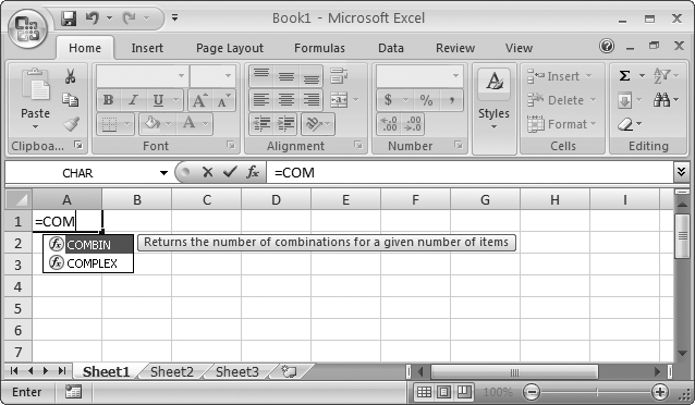
Figure 15-3. After you type =COM, Excel helpfully points out that it knows only two functions that start that way: COMBIN( ) and COMPLEX( ). If your fingers are getting tired, then use the arrow keys o pick the right one out of the list, and then click Tab to pop it into your formula. (Or, you can just double-click it with the mouse.)
In the case of the COMBIN( ) function, Excel needs two pieces of information, or arguments. The first is the number of items in the set (the 52-card deck), and the second’s the number of items you’re randomly selecting (in this case, 5). Most functions, like COMBIN( ), require two or three arguments. However, some functions can accept many more, while a few don’t need any arguments at all. Once again, Formula AutoComplete guides you by telling you what arguments you need, as shown in Figure 15-4.
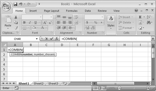
Figure 15-4. When you type the opening parentheses after a function name, Excel automatically displays a tooltip indicating what arguments the function requires. The argument you’re currently entering is shown bolded in the tooltip. The argument names aren’t crystal clear, but if you already know how the function works, they’re usually enough to jog your memory.
Once you’ve typed this formula into a cell, the result (2598960) appears in your worksheet. In other words, there are 2,598,960 different possible five-card combinations in any deck of cards. Rather than having to calculate this fact using probability theory—or, heaven forbid, trying to count out the possibilities manually—the COMBIN( ) function handled it for you.
Note
Even if a function doesn’t take any arguments, you still need to supply an empty set of parentheses after the function name. One example is the RAND( ) function, which generates a random fractional number. The formula =RAND( ) works fine, but if you forget the parentheses and merely enter =RAND, then Excel displays an error message (#NAME?) that’s Excelian for: “Hey! You got the function’s name wrong.” See Table 15-2 on Logical Operators for more information about Excel’s error messages.
One of the particularly powerful things about functions is that they don’t necessarily need to use literal values in their arguments. They can also use cell references. For example, you could rewrite the five-card combination formula (mentioned previously) so that it specifies the number of cards that’ll be drawn from the deck based on a number that you’ve typed in somewhere else in the spreadsheet.
Assuming this information’s entered into cell B2, the formula would become:
| =COMBIN(52,B2) |
Building on this formula, you can calculate the probability (albeit astronomically low) of getting the exact hand you want in one draw:
| =1/COMBIN(52,B2) |
You could even multiply this number by 100 or use the Percent number style to see your percentage chance of getting the cards you want.
In many cases, you don’t want to refer to just a single cell, but rather a range of cells. A range is simply a grouping of multiple cells. These cells may be next to each other (say, a range that includes all the cells in a single column), or they could be scattered across your worksheet. Ranges are useful for computing averages, totals, and many other calculations.
To group together a series of cells, use one of the two following reference operators:
The comma (,) separates more than one cell. For example, the series A1, B7, H9 is a cell range that contains three cells. The comma’s known as the union operator. You can add spaces before or after a comma, but Excel just ignores or removes them (depending on its mood).
The colon (:) separates the top-left and bottom-right corners of a block of cells. You’re telling Excel: “Hey, use this block of cells in my formula.” For example, A1:A5 is a range that includes cells A1, A2, A3, A4, and A5. The range A2:B3 is a grid that contains cells A2, A3, B2, and B3. The colon is the range operator—by far the most powerful way to select multiple cells.
Tip
As you might expect, Excel lets you specify ranges by selecting cells with your mouse, instead of typing in the range manually. You’ll see this trick later in this chapter on Formula Shortcuts.
You can’t enter ranges directly into formulas that just use the simple operators. For example, the formula =A1:B1+5 doesn’t work, because Excel doesn’t know what to do with the range A1:B1. (Should the range be summed up? Averaged? Excel has no way of knowing.) Instead, you need to use ranges with functions that know how to use them. For instance, one of Excel’s most basic functions is named SUM( ); it calculates the total for a group of cells. To use the SUM( ) function, you enter its name, an open parenthesis, the cell range you want to add up, and then a closed parenthesis.
Here’s how you can use the SUM( ) function to add together three cells, A1, A2, and A3:
| =SUM(A1,A2,A3) |
And here’s a more compact syntax that performs the same calculation using the range operator:
| =SUM(A1:A3) |
A similar SUM( ) calculation’s shown in Figure 15-5. Clearly, if you want to total a column with hundreds of values, then it’s far easier to specify the first and last cell using the range operator rather than including each cell reference in your formula!
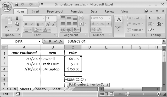
Figure 15-5. Using a cell range as the argument in the SUM( ) function is a quick way to add up a series of numbers in a column. Note that when you enter or edit a formula, Excel highlights all the cells that formula uses with different colored borders. In this example, you see the range of cells C2, C3, and C4 in a blue box.
If you make a syntax mistake when entering a formula (such as leaving out a function argument or including a mismatched number of parentheses), Excel lets you know right away. Moreover, like a stubborn school teacher, Excel won’t accept the formula until you’ve corrected it. It’s also possible, though, to write a perfectly legitimate formula that doesn’t return a valid answer. Here’s an example:
| =A1/A2 |
If both A1 and A2 have numbers, this formula works without a hitch. However, if you leave A2 blank, or if you enter text instead of numbers, then Excel can’t evaluate the formula, and it reminds you with an error message.
Excel lets you know about formula errors by using an error code that begins with the number sign (#) and ends with an exclamation point (!), as shown in Figure 15-6. In order to remove this error, you need to track down the problem and resolve it, which may mean correcting the formula or changing the cells it references.
When you click the exclamation mark icon next to an error, you see a menu of choices (as shown in Figure 15-6):
Help On This Error pops open Excel’s online help, with a (sometimes cryptic) description of the problem and what could have caused it.
Show Calculation Steps pops open the Evaluate Formula dialog box, where you can work your way through a complex formula one step at a time.
Ignore Error tells Excel to stop bothering you about this problem, in any worksheet you create. You won’t see the green triangle for this error again (although you’ll still see the error code in the cell).
Edit in Formula Bar brings you to the formula bar, where you can change the formula to fix a mistake.
Error Checking Options opens up the Excel Options dialog box, and brings you to the section where you can configure the settings Excel uses for alerting you about errors. You can turn off background error checking, or change the color of the tiny error triangles using the settings under the Error Checking heading. (Background error checking is the feature that flags cells with tiny green triangles when the cells contain a problem.) You can also tell Excel to start paying attention to errors you previously told it ignore by clicking the Reset Ignored Errors button.

Figure 15-6. When Excel spots an error, it inserts a tiny green triangle into the cell’s top-left corner. When you move to the offending cell, Excel displays an exclamation mark icon next to it (a smart tag). Hover over the exclamation mark to view a description of the error (which appears in a tooltip), or click the exclamation icon to see a list of menu options.
Table 15-2 lists most of the error codes that Excel uses.
Table 15-2. Excel’s Error Codes
So far, you’ve seen the basic arithmetic operators (which are used for addition, subtraction, division, and so on) and the cell reference operators (used to specify one or more cells). There’s one final category of operators that’s useful when creating formulas: logical operators.
Logical operators let you build conditions into your formulas so the formulas produce different values depending on the value of the data they encounter. You can use a condition with cell references or literal values.
For example, the condition A2=A4 is true if cell A2 contains the same value as cell A4. On the other hand, if these cells contain different values (say 2 and 3), then the formula generates a false value. Using conditions is a stepping stone to using conditional logic. Conditional logic lets you perform different calculations based on different scenarios.
For example, you can use conditional logic to see how large an order is, and provide a discount if the total order cost’s over $5,000. Excel evaluates the condition, meaning it determines if the condition’s true or false. You can then tell Excel what to do based on that evaluation.
Table 15-3 lists all the logical operators you can use to build formulas.
Table 15-3. Logical Operators
|
Operator |
Name |
Example |
Result |
|---|---|---|---|
|
= |
Equal to |
1=2 |
FALSE |
|
> |
Greater than |
1>2 |
FALSE |
|
< |
Less than |
1<2 |
TRUE |
|
>= |
Greater than or equal to |
1>=1 |
TRUE |
|
<= |
Less than or equal to |
1<=1 |
TRUE |
|
<> |
Not equal to |
1<>1 |
FALSE |
You can use logical operators to build standalone formulas, but that’s not particularly useful. For example, here’s a formula that tests whether cell A1 contains the number 3:
| =(A2=3) |
The parentheses aren’t actually required, but they make the formula a little bit clearer, emphasizing the fact that Excel evaluates the condition first, and then displays the result in the cell. If you type this formula into the cell, then you see either the uppercase word TRUE or FALSE, depending on the content in cell A2.
On their own, logical operators don’t accomplish much. However, they really shine when you start combining them with other functions to build conditional logic. For example, you can use the SUMIF( ) function, which totals the value of certain rows, depending on whether the row matches a set condition. Or you can use the IF( ) function to determine what calculation you should perform.
The IF( ) function has the following function description:
| IF(condition, [value_if_true], [value_if_false]) |
In English, this line of code translates to: If the condition is true, display the second argument in the cell; if the condition is false, display the third argument.
Consider this formula:
| =IF(A1=B2, “These numbers are equal”, “These numbers are not equal”) |
This formula tests if the value in cell A1 equals the value in cell B2. If this is true, you’ll see the message “These numbers are equal” displayed in the cell. Otherwise, you’ll see “These numbers are not equal.”
Note
If you see a quotation mark in a formula, it’s because that formula uses text. You must surround all literal text values with quotation marks. (Numbers are different: You can enter them directly into a formula.)
People often use the IF( ) function to prevent Excel from performing a calculation if some of the data is missing. Consider the following formula:
| =A1/A2 |
This formula causes a divide-by-zero error if A2 contains a 0 value. Excel then displays an error code in the cell. To prevent this from occurring, you can replace this formula with the conditional formula shown here:
| =IF(A2=0, 0, A1/A2) |
This formula checks if cell A2 is empty or contains a 0. If so, the condition is true, and the formula simply gives you a 0. If it isn’t, the condition is false, and Excel performs the calculation A1/A2.
So far, you’ve learned how to build a formula by entering it manually. That’s a good way to start out because it forces you to understand the basics of formula writing. But writing formulas by hand is a drag; plus, it’s easy to type in the wrong cell address. For example, if you type A2 instead of A3, you can end up with incorrect data, and you won’t necessarily notice your mistake.
As you become more comfortable with formulas, you’ll find that Excel gives you a few tools—like point-and-click formula creation and the Insert Function button—to speed up your formula writing and reduce your mistakes. You’ll learn about these features in the following sections.
Note
In previous versions of Excel, the Insert Function dialog box was almost exactly the same, except it was known as the Function wizard.
Instead of entering a formula by typing it out letter-by-letter, Excel lets you create formulas by clicking the cells you want to use. For example, consider this simple formula that totals the numbers in two cells:
| =A1+A2 |
To build this formula by clicking, just follow these steps:
Move to the cell where you want to enter the formula.
This cell’s where the result of your formula’s calculation will appear. While you can pick any cell on the worksheet, A3 works nicely because it’s directly below the two cells you’re adding.
Press the equal sign (=) key.
Move to the first cell you want to use in your formula (in this case, A1).
You can move to this first cell by pressing the up arrow key twice, or by clicking it with the mouse. You’ll notice that moving to another cell doesn’t cancel your edit, as it would normally, because Excel recognizes that you’re building a formula. When you move to the new cell, the cell reference appears automatically in the formula (which Excel displays in cell A3, as well as in the formula bar just above your worksheet). If you move to another cell, Excel changes the cell reference accordingly.
Press the + key.
Excel adds the + sign to your formula so that it now reads =A1+.
Finish the formula by moving to cell A2 and pressing Enter.
Again, you can move to A2 either by pressing the up arrow key or by clicking the cell directly. Remember, you can’t just finish the formula by moving somewhere else; you need to press Enter to tell Excel you’re finished writing the formula. Another way to complete your edit is to click the checkmark that appears on the formula bar, to the left of the current formula. Even experienced Excel fans get frustrated with this step. If you click another cell before you press Enter, then you won’t move to the cell—instead, Excel inserts the cell into your formula.
Tip
You can use this technique with any formula. Just type in the operators, function names, and so on, and use the mouse to select the cell references. If you need to select a range of cells, then just drag your mouse until the whole group of cells is highlighted. You can practice this technique with the SUM( ) function. Start by typing =SUM( into the cell, and then selecting the range of cells you want to add. Finish by adding a final closing parenthesis and pressing Enter.
You can use a similar approach to edit formulas, although it’s slightly trickier:
Move to the cell that contains the formula you want to edit, and put it in edit mode by double-clicking it or pressing F2.
Excel highlights all the cells that this formula uses with a colored outline. Excel’s even clever enough to use a helpful color-coding system. Each cell reference uses the same color as the outline surrounding the cell it’s referring to. This can help you pick out where each reference is.
Click the outline of the cell you want to change. (Your pointer changes from a fat plus sign to a four-headed arrow when you’re over the outline.) With the mouse button still held down, drag this outline over to the new cell (or cells) you want to use.
Excel updates the formula automatically. You can also expand and shrink cell range references. To do so, put the formula-holding cell into edit mode, and then click any corner of the border that surrounds the range you want to change. Next, drag the border to change the size of the range. If you want to move the range, then click any part of the range border and drag the outline in the same way as you would with a cell reference.
Press Enter or click the formula bar checkmark to accept your changes.
That’s it.
The ribbon is stocked with a few buttons that make formula writing easier. To take a look, click the Formulas tab.
The most important part of the Formulas tab is the Function Library section at the left. It includes the indispensable Insert Function button, which you’ll take for a spin in the next section. It also includes many more buttons that arrange Excel’s vast catalog of functions into related categories for easier access. Figure 15-7 shows how it works.
The Function Library divides its functions into the following categories:
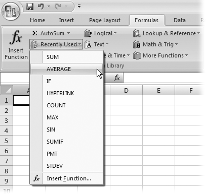
AutoSum has a few shortcuts that let you quickly add, average, or otherwise deal with a list of numbers.
Recently Used has exactly what you’d expect—functions that you’ve recently chosen from the Function Library. If you’re just starting out with functions, you see that Excel fills the Recently Used list with a small set of commonly used functions, like SUM( ).
Figure 15-7. Each button in the Function Library section (other than Insert Function) pops up a mini menu of function choices. Choose one, and Excel inserts that function into the current formula. You can use this technique to find functions that you’ve used recently, or to browse the main function categories.
Financial functions let you track your car loan payments and calculate how many more years until you can retire rich.
Logical functions let you create conditional logic for even smarter spreadsheets that make calculation decisions.
Text functions manipulate words, sentences, and other non-numeric information.
Date & Time functions perform calendar math and can help you sort out ages, due dates, and more.
Lookup & Reference functions perform the slightly mind-bending feat of searching for information in other cells.
Math & Trig functions are the mathematic basics, including sums, rounding, and all the other high-school trigonometry you’re trying to forget.
More Functions groups together some heavy-duty Excel functions that are intended for specialized purposes. This category includes high-powered statistical and engineering functions.
Excel provides more than 300 built-in functions. In order to use a function, however, you need to type its name in exactly. That means that every time you want to employ a function, you’ll need to refer to this book, call on your own incredible powers of recollection, or click over to the convenient Insert Function button.
To use the Insert Function feature, choose Formulas → Function Library → Insert Function. However, formula pros skip straight to the action by clicking the fx button that appears just to the left of the formula bar. (Or, they press the Shift+F3 shortcut key.)
No matter which approach you use, Excel displays the Insert Function dialog box (shown in Figure 15-8), which offers three ways to search for and insert any of Excel’s functions.
If you’re looking for a function, the easiest way to find one is to choose a category from the “Or select a category” drop-down list. For example, when you select the Math & Trig category, you see a list of functions with names like SIN( ) and COS( ), which perform basic trigonometric calculations.
If you choose the Most Recently Used category, you’ll see a list of functions you’ve recently picked from the ribbon or the Insert Function dialog box.
If you’re really ambitious, you can type a couple of keywords into the “Search for a function” text box. Next, click Go to perform the search. Excel gives you a list of functions that match your keywords.
Figure 15-8. Top: The Insert Function dialog box lets you quickly find the function you need. You can choose a category that seems likely to have the functions you’re interested in. Bottom: You can also try to search by entering keywords in the “Search for a function” box. Either way, when you click one of the functions in the list, Excel presents you with a description of the function at the bottom of the window.

When you spot a function that looks promising, click it once to highlight its name. Excel then displays a brief description of the function at the bottom of the window. For more information, you can click the “Help on this function” link in the bottom-left corner of the window. To build a formula using this function, click OK.
Excel then inserts the function into the currently active cell, followed by a set of parentheses. Next, it closes the Insert Function dialog box and opens the Function Arguments dialog box (Figure 15-9).
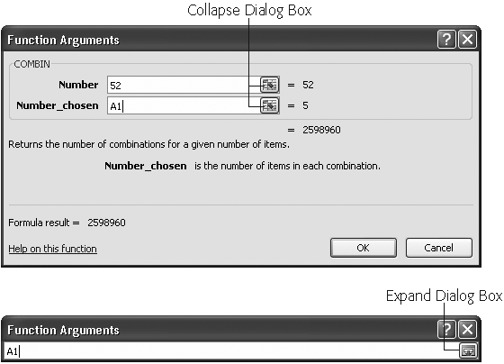
Figure 15-9. Top: Here, the COMBIN( ) function has just been inserted via the Insert Function dialog box. Because the COMBIN( ) function requires two arguments (Number and Number_ chosen), the Function Arguments dialog box shows two text boxes. The first argument uses a literal value (52), while the second argument uses a cell reference (A1). As you enter the arguments, Excel updates the formula in the worksheet’s active cell, and displays the result of the calculation at the bottom of the Function Arguments dialog box. Bottom: If you need more room to see the worksheet and select cells, you can click the Collapse Dialog Box icon to reduce the window to a single text box. Clicking the Expand Dialog Box icon restores the window to its normal size.
Note
Depending on the function you’re using, Excel may make a (somewhat wild) guess about which arguments you want to supply. For example, if you use the Insert Function window to add a SUM( ) function, then you’ll see that Excel picks a nearby range of cells. If this isn’t what you want, just replace the range with the correct values.
Now you can finish creating your formula by using the Function Arguments dialog box, which includes a text box for every argument in the function. It also includes a help link for detailed information about the function, as shown in Figure 15-10.
To complete your formula, follow these steps:
Click the text box for the first argument.
A brief sentence describing the argument appears in the Function Arguments dialog box.
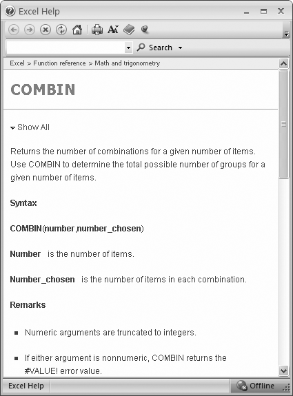
Figure 15-10. Both the Insert Function and Function Arguments dialog boxes make it easy to get detailed reference information about any function by clicking the “Help on this function” link at the bottom left of the window. The help page shown here shows the reference for the COMBIN( ) function.
Some functions don’t require any arguments. In this case, you don’t see any text boxes, although you still see some basic information about the function. Skip directly to step 4.
Enter the value for the argument.
If you want to enter a literal value (like the number 52), type it in now. To enter a cell reference, you can type it in manually, or click the appropriate cell on the worksheet. To enter a range, drag the cursor to select a group of cells.
You may need to move the Function Arguments dialog box to the side to expose the part of the worksheet you want to click. The Collapse Dialog Box icon (located to the immediate right of each text box) is helpful since clicking it shrinks the window’s size. This way, you’ll have an easier time selecting cells from your worksheet. To return the window to normal, click the Expand Dialog Box icon, which is to the right of the text box.
Repeat step 2 for each argument in the function.
As you enter the arguments, Excel updates the formula automatically.
Once you’ve specified a value for every required argument, click OK.
Sometimes you need to perform similar calculations in different cells throughout a worksheet. For example, say you want to calculate sales tax on each item in a product catalog, the monthly sales in each store of a company, or the final grade for each student in a class. In this section, you’ll learn how Excel makes it easy with relative cell references. Relative cell references are cell references that Excel updates automatically when you copy them from one cell into another. They’re the standard kind of references that Excel uses (as opposed to absolute cell references, which are covered in the next section). In fact, all the references you’ve used so far have been relative references, but you haven’t yet seen how they work with copy-and-paste operations.
Consider the worksheet shown in Figure 15-11, which contains a teacher’s grade book. In this example, each student has three grades: two tests and one assignment. A student’s final grade is based on the following percentages: 25 percent for each of the two tests, and 50 percent for the assignment.
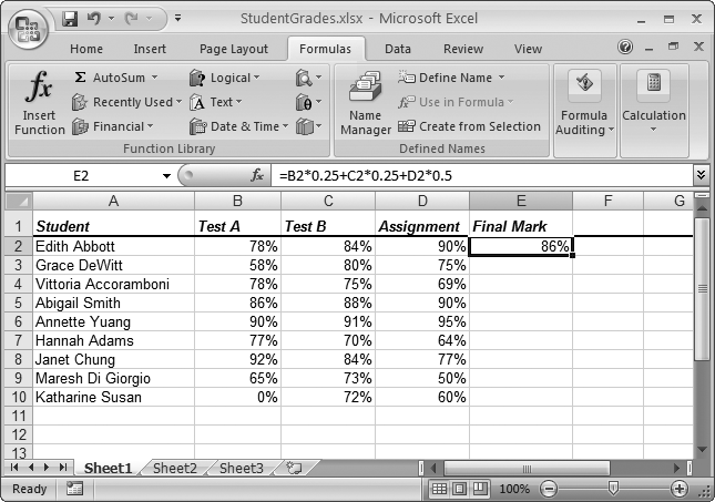
Figure 15-11. This worksheet shows a list of students in a class, and calculates the final grade for each student using two test scores and an assignment score. So far, the only formula that’s been added is for the first student (in cell E2).
The following formula calculates the final grade for the first student (Edith Abbott):
| =B2*25% + C2*25% + D2*50% |
The formula that calculates the final mark for the second student (Grace DeWitt) is almost identical. The only change is that all the cell references are offset by one row, so that B2 becomes B3, C2 becomes C3, and D2 becomes D3:
| =B3*25% + C3*25% + D3*50% |
You may get fed up entering all these formulas by hand. A far easier approach is to copy the formula from one cell to another. Here’s how:
Move to the cell containing the formula you want to copy.
In this example, you’d move to cell E2.
Copy the formula to the clipboard by pressing Ctrl+C.
You can also copy the formula by choosing Home → Clipboard → Copy.
Select the range of cells you want to copy the formula into.
Select cells E3 to E10.
Paste in the new formulas by pressing Ctrl+V.
You can also paste the formula by choosing Home → Clipboard → Paste.
When you paste a formula, Excel magically copies an appropriate version of the formula into each of the cells from E3 to E10. These automatic formula adjustments occur for any formula, whether it uses functions or just simple operators. Excel then automatically calculates and displays the results, as shown in Figure 15-12.

Tip
There’s an even quicker way to copy a formula to multiple cells by using the AutoFill feature introduced in Chapter 10. In the student grade example, you’d start by moving to cell E2, which contains the original formula. Then, you’d click the small square at the bottom-right corner of the cell outline, and drag the outline down until it covers all cells from E3 to E10. When you release the mouse button, Excel inserts the formula copies in the AutoFill region.
Relative references are a true convenience since they let you create formula copies that don’t need the slightest bit of editing. But you’ve probably already realized that relative references don’t always work. For example, what if you have a value in a specific cell that you want to use in multiple calculations? You may have a currency conversion ratio that you want to use in a list of expenses. Each item in the list needs to use the same cell to perform the conversion correctly. But if you make copies of the formula using relative cell references, then you’ll find that Excel adjusts this reference automatically and the formula ends up referring to the wrong cell (and therefore the wrong conversion value).
Figure 15-13 illustrates the problem with the worksheet of student grades. In this example, the test and assignment scores aren’t all graded out of 100 possible points; each item has a different total score available (listed in row 12). In order to calculate the percentage a student earned on a test, you need to divide the test score by the total score available. This formula, for example, calculates the percentage for Edith Abbott’s performance on Test B:
| =B2/B12*100% |

Figure 15-13. In this version of the student grade book, both the tests and the assignment are graded on different scales (as listed in row 12). When you copy the Final Grade formula from the first row (cell E2) to the rows below it, Excel offsets the formula to use B13, C13, and D13—none of which provide any information. Thus a problem occurs—shown here as a divide-by-zero error. To fix this, you need to use absolute cell references.
To calculate Edith’s final grade for the class, you’d use the following formula:
| =B2/B12*25% + C2/C12*25% + D2/D12*50% |
Like many formulas, this one contains a mix of cells that should be relative (the individual scores in cells B2, C2, and D2) and those that should be absolute (the possible totals in cell B12, C12, and D12). As you copy this formula to subsequent rows, Excel incorrectly changes all the cell references, causing a calculation error.
Fortunately, Excel provides a perfect solution. It lets you use absolute cell references—cell references that always refer to the same cell. When you create a copy of a formula that contains an absolute cell reference, Excel doesn’t change the reference (as it does when you use relative cell references; see the previous section). To indicate that a cell reference is absolute, use the dollar sign ($) character. For example, to change B12 into an absolute reference, you would add the $ character twice, once in front of the column and once in front of the row, which changes it to $B$12.
Here’s the corrected class grade formula (for Edith) using absolute cell references:
| =B2/$B$12*25% + C2/$C$12*25% + D2/$D$12*50% |
This formula still produces the same result for the first student. However, you can now copy it correctly for use with the other students. To copy this formula into all the cells in column E, use the same procedure described in the previous section on relative cell references.
You might wonder why you need to use the $ character twice in an absolute reference (before the column letter and the row number). The reason is that Excel lets you create partially fixed references. To understand partially fixed references, it helps to remember that every cell reference consists of a column letter and a row number. With a partial fixed reference, Excel updates one component (say, the column part) but not the other (the row) when you copy the formula. If this sounds complex (or a little bizarre), consider a few examples:
You have a loan rate in cell A1, and you want all loans on an entire worksheet to use that rate in calculations. If you refer to the cell as $A$1, then its column and row always stay the same when you copy the formula to another cell.
You have several rows of loan information. The first column of a row always contains the loan rate for all loans on that row. In your formula cell, if you refer to cell $A1, then when you copy the formula across columns and rows, the row changes (2, 3, 4, etc.) but the column doesn’t (A2, A3, A4, etc.).
You have a table of loan rates organized by the length of the loan (10-year, 15-year, 20-year, etc.) along the top of a worksheet. Loans in each column are calculated using the rate specified at the top of that column. If you refer to the rate cell as A$1 in your first column’s formula, then the row stays constant (1), but the column changes (B1, C1, D1, etc.) as you copy the formula across columns and down rows.
Tip
You can quickly change formula references into absolute or partially fixed references. Just put the cell into edit mode (by double-clicking it or pressing F2). Then, move through the formula until you’ve highlighted the appropriate cell reference. Now, press F4 to change the cell reference. Each time you press F4, the reference changes. If the reference is A1, for instance, it becomes $A$1, then A$1, then $A1, and then A1 again.