The previous chapters have given you all the tools you need to create nicely formatted worksheets. While this is all well and good, these features can quickly bury you in an avalanche of data. If you want to see more than one part of your workbook at once, or if you want an overview of the entire worksheet, then you have to seize control of Excel’s viewing features.
These features include zooming (which lets you magnify cells or just fit more information into your Excel window), panes (which let you see more than one part of a worksheet at once), and freezing (which lets you keep certain cells visible at all times). This chapter teaches you how to use all these tools, and how to store a custom view so your spreadsheet looks just the way you want it.
No matter what your worksheets look like on a screen, sometimes the best way to review them is in print. The second half of this chapter tackles printing your worksheets. You’ll learn Excel’s basic printing options and a few tricks that can help you preview page breaks and make sure large amounts of data get divided the way you want.
So far, most of the worksheets in this book have included only a small amount of data. But as you cram your worksheets with dozens of columns, and hundreds or even thousands of rows, editing becomes much trickier. The most challenging problems are keeping track of where you are in an ocean of information and making sure the data you want stays visible. Double that if you have multiple large worksheets in one workbook.
The following sections introduce the basic tools you can use to view your data, along with a few tips for managing large worksheets.
Excel’s zoom feature lets you control how much data you’ll see in the window. When you reduce the zoom percentage—say from 100 percent to 10 percent—Excel shrinks your individual cells, letting you see more of them at once, which also makes it harder to read the data. Very small zoom percentages are ideal for looking at the overall layout of a worksheet. When you increase the zoom percentage—say from 100 percent to 200 percent—Excel magnifies your cells, letting you see more detail but fewer cells. Larger zoom percentages are good for editing.
You can most easily adjust the zoom percent by using the zoom slider in the bottom-right part of the status bar. The zoom slide also displays the current zoom percentage. But if you want to specify the exact zoom percentage by hand (say, 142 percent), then you can choose View → Zoom → Zoom. A Zoom dialog box appears (Figure 14-1).

Figure 14-1. Left: Using the Zoom dialog box, you can select a preset zoom percentage or, in the Custom box, type in your own percentage. Right: But using the Zoom slider is almost always faster than making frequent trips to the Zoom dialog box.
The standard zoom setting is 100 percent, although other factors like the size of the font you’re using and the size and resolution of your computer screen help determine how many cells fit into Excel’s window. As a rule of thumb, every time you double the zoom, Excel cuts in half the number of rows you can see. Thus, if you can see 20 rows at 100 percent, then you’ll see 10 rows at 200 percent.
Note
Changing the zoom affects how your data appears in the Excel window, but it won’t have any effect on how your data is printed or calculated.
You can also zoom in on a range of cells. When your data extends beyond the edges of your monitor, this handy option lets you shrink a portion to fit your screen. Conversely, if you’ve zoomed out to get a bird’s eye view of all your data, and you want to swoop in on a particular section, Excel lets you expand a portion to fit your screen. To zoom in on a group of cells, first select some cells (Figure 14-2), and then choose View → Zoom → Zoom to Selection (Figure 14-3). (You can perform this same trick by highlighting some cells, opening the Zoom dialog box, and then choosing "Fit selection.”) Make sure you select a large section of the worksheet—if you select a small group, you’ll end up with a truly jumbo-sized zoom.

Figure 14-2. To magnify a range of cells, select them, as shown here, and then choose View → Zoom → Zoom to Selection to have Excel expand the range to fill the entire window, as shown in Figure 14-3.

Zooming is an excellent way to survey a large expanse of data or focus on just the important cells, but it won’t help if you want to simultaneously view cells that aren’t near each other. For example, if you want to focus on both row 1 and row 138 at the same time, then zooming won’t help. Instead, try splitting your Excel window into multiple panes—separate frames that each provide a different view of the same worksheet. You can split a worksheet into two or four panes, depending on how many different parts you want to see at once. When you split a worksheet, each pane contains an identical replica of the entire worksheet. When you make a change to the worksheet in one pane, Excel automatically applies the same change in the other panes. The beauty of panes is that you can look at different parts of the same worksheet at once.
You can split a window horizontally or vertically (or both). When you want to compare different rows in the same worksheet, use a horizontal split. To compare different columns in the same worksheet, use a vertical split. And if you want to be completely crazy and see four different parts of your worksheet at once, then you can use a horizontal and a vertical split—but that’s usually too confusing to be much help.
Excel gives you two ways to split the windows. Here’s the easy way:
Find the splitter controls on the right side of the screen.
Figure 14-4 shows you where to find them.
Drag either control to split the window into two panes. As you drag, Excel displays a gray bar showing where it’ll divide the window. Release the splitter control when you’re happy with the layout. (At this point, you don’t need to worry about whether you can actually view the data you want to compare; you’re simply splitting up the window.)
If you want to split the window into an upper and lower portion, drag the horizontal control down to the location where you want to split the window.
If you want to split the window into a left and right portion, drag the vertical control leftwards—to the location where you want to split the window.
Note
If for any reason you do want to split the window into four panes, use both controls. The order you follow isn’t important.
If you don’t like the layout you’ve created, simply move the splitter bars by dragging them just as you did before.
Within each pane, scroll to the cells you want to see.
For example, if you have a 100-row table that you split horizontally in order to compare the top five rows and the bottom five, scroll to the top of the upper pane, and then scroll to the bottom of the lower pane. (Again, the two panes are replicas of each other; Excel is just showing you different parts of the same worksheet.)
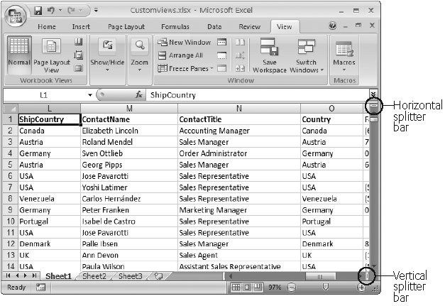
Using the scroll bars in panes can take some getting used to. When the window is split in two panes, Excel synchronizes scrolling between both panes in one direction. For example, if you split the window into top and bottom halves, Excel gives you just one horizontal scroll bar (at the bottom of the screen), which controls both panes (Figure 14-5). Thus, when you scroll to the left or right, Excel moves both panes horizontally. On the other hand, Excel gives you separate vertical scroll bars for each pane, letting you independently move up and down within each pane.
Tip
If you want the data in one pane—for example, column titles—to remain in place, you can freeze that pane. The next section tells you how.
The reverse is true with a vertical split; in this case, you get one vertical scroll bar and two horizontal bars, and Excel synchronizes both panes when you move up or down. With four panes, life gets a little more complicated. In this case, when you scroll left or right, the frame that’s just above or just below the current frame moves, too. When you scroll up or down, the frame that’s to the left or to the right moves with you. Try it out.
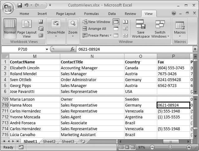
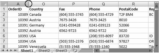
Figure 14-5. Here you can see the data in rows 1 through 6 and rows 709 through 715 at the same time. As you move from column to column, both panes move in sync, letting you see, for instance, the phone number information in both panes at once. (You can scroll up or down separately in each pane.)
Note
If you want to remove your panes, then just drag the splitter bars back to the edges of the window, or double-click it.
You can also create panes by using the ribbon command View → Window → Split. When you do, Excel carves the window into four equal panes. You can change the pane sizes as described above, or use View → Window → Split again to return to normal.
Excel has another neat trick up its sleeve to help you manage large worksheets: freezing. Freezing is a simpler way to make sure a specific set of rows or columns remains visible at all times. When you freeze data, it remains fixed in place in the Excel window, even as you move to another location in the worksheet in a different pane. For example, say you want to keep visible the first row that contains column titles. When you freeze that row, you can always tell what’s in each column—even when you’ve scrolled down several screenfuls. Similarly, if your first column holds identifying labels, you may want to freeze it so that when you scroll off to the right, you don’t lose track of what you’re looking at.
Tip
Excel lets you print out worksheets with a particular row or column fixed in place. Paper size and orientation tells you how.
You can freeze rows at the top of your worksheet, or columns at the left of your worksheet, but Excel does limit your freezing options in a few ways:
You can freeze rows or columns only in groups. That means you can’t freeze column A and C without freezing column B. (You can, of course, freeze just one row or column.)
Freezing always starts at column A (if you’re freezing columns) or row 1 (if you’re freezing rows). That means that if you freeze row 13, Excel also freezes all the rows above it (1 through 12) at the top of your worksheet.
If a row or column isn’t visible and you freeze it, you can’t see it until you unfreeze it. For example, if you scroll down so that row 100 appears at the top of the worksheet grid, and then freeze the top 100 rows, you can’t see rows 1 to 99 anymore. This may be the effect you want, or it may be a major annoyance.
Note
As far as Excel is concerned, frozen rows and columns are a variation on panes (described earlier). When you freeze data, Excel creates a vertical pane for columns or a horizontal pane for rows. It then fixes that pane so you can’t scroll through it.
To freeze a row or set of rows at the top of your worksheet, just follow these steps:
Make sure the row or rows you want to freeze are visible and at the top of your worksheet.
For example, if you want to freeze rows 2 and 3 in place, make sure they’re visible at the top of your worksheet. Remember, rows are frozen starting at row 1. That means that if you scroll down so that row 1 isn’t visible, and you freeze row 2 and row 3 at the top of your worksheet, then Excel also freezes row 1—and keeps it hidden so you can’t scroll up to see it.
Move to the first row you want unfrozen, and then move left to column A.
At this point, you’re getting into position so that Excel knows where to create the freeze.
Select View → Freeze Panes → Freeze Panes.
Excel splits the worksheet, but instead of displaying a gray bar (as it does when you create panes), it uses a solid black line to divide the frozen rows from the rest of the worksheet. As you scroll down the worksheet, the frozen rows remain in place.
To unfreeze the rows, just select View → Freeze Panes → Unfreeze Panes.
Freezing columns works the same way:
Make sure the column or columns you want to freeze are visible and at the left of your worksheet.
For example, if you want to freeze columns B and C in place, make sure they’re visible at the edge of your worksheet. Remember, columns are frozen starting at column A. That means that if you scroll over so that column A isn’t visible, and you freeze columns B and C on the left side of your worksheet, Excel also freezes column A—and keeps it hidden so you can’t scroll over to see it.
Move to the first column you want unfrozen, and then move up to row 1.
At this point, you’re getting into position so that Excel knows where to create the freeze.
Select View → Freeze Panes → Freeze Panes.
Excel splits the worksheet, but instead of displaying a gray bar (as it does when you create panes), Excel uses a solid black line to divide the frozen columns from the rest of the worksheet. As you scroll across the worksheet, the frozen columns remain in place.
To unfreeze the columns, select View → Freeze Panes → Unfreeze Panes.
Tip
If you’re freezing just the first row or the leftmost column, then there’s no need to go through this whole process. Instead, you can use the handy View → Freeze Panes → Freeze Top Row or View → Freeze Panes → Freeze First Column.
You can also freeze columns and rows at the same time, which is useful when you have identifying information that you need to keep visible both on the left and the top of your worksheet. Figure 14-6 shows an example.
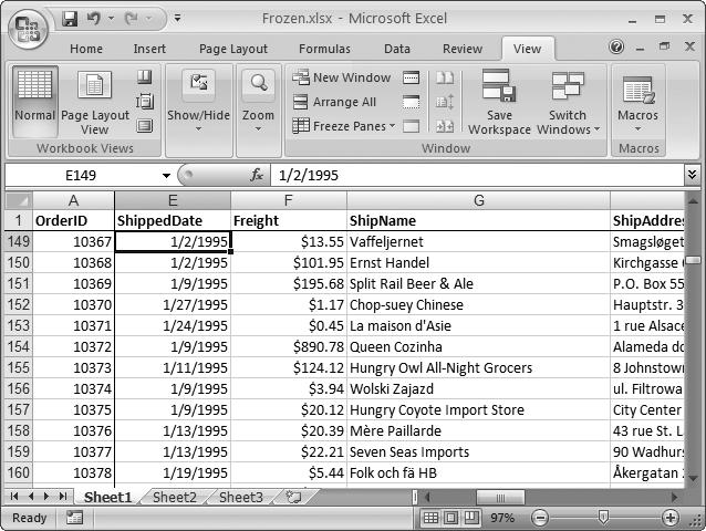
Figure 14-6. Here, both column A and row 1 are frozen, and thus always remain visible. The easiest way to create these frozen regions is to scroll to the top of the worksheet, position the active cell at B2, and choose View → Freeze Panes → Freeze Panes. Excel then automatically freezes the rows above and the columns to the left in separate panes.
In some cases your problem isn’t that you need to keep data visible, but that you need to hide it. For example, say you have a column of numbers that you need only for a calculation but don’t want to see when you edit or print the sheet. Excel provides the perfect solution: hiding rows and columns. Hiding doesn’t delete information, it just temporarily tucks it out of view. You can restore hidden information any time you need it.
Technically, hiding a row or column is just a special type of resizing. When you instruct Excel to hide a column, it simply shrinks the column down to a width of 0. Similarly, when you hide a row, Excel compresses the row height.
You can hide data a few ways:
To hide a column, right-click the column header (the letter button on the top of the column), and then choose Hide. Or, put your cursor in any row in that column, and then select Home → Cells → Format → Hide & Unhide → Hide Columns.
To hide a row, right-click the row header (the number button at the left of the row), and then choose Hide. Or, put your cursor in any column in that row, and then select Home → Cells → Format → Hide & Unhide → Hide Rows.
To hide multiple rows or columns, just select all the ones you want to disappear before choosing Hide.
To unhide a column or row, select the range that includes the hidden cells. For example, if you hid column B, select columns A and C by dragging over the numeric row headers. Then choose Home → Cells → Format → Hide & Unhide → Unhide Columns (or Unhide Rows). Or just right-click the selection, and then choose Unhide. Either way, Excel makes the missing columns or rows visible and then highlights them so you can see which information you’ve restored.
Tip
To unhide all columns (or rows) in a worksheet, select the entire worksheet (by clicking the square in the top-left corner of the grid), and then select Home → Cells → Format → Hide & Unhide → Unhide Columns (or Unhide Rows).
Forgetting that you’ve hidden data is as easy as forgetting where you put your keys. While Excel doesn’t include a hand-clapper to help you locate your cells, it does indicate that some of your row numbers or column letters are missing, as shown in Figure 14-7.
If you regularly tweak things like the zoom, visible columns, and the number of panes, you can easily spend more time adjusting your worksheet than editing it. Fortunately, Excel lets you save your view settings with custom views. Custom views let you save a combination of view settings in a workbook. You can store as many custom views as you want. When you want to use a particular view you’ve created, simply select it from a list and Excel applies your settings.
Custom views are particularly useful when you frequently switch views for different tasks, like editing and printing. For example, if you like to edit with several panes open and all your data visible, but you like to print your data in one pane with some columns hidden, custom views let you quickly switch between the two layouts.
Custom views can save the following settings:
The location of the active cell. (In other words, your position in the worksheet. For example, if you’ve scrolled to the bottom of a 65,000-row spreadsheet, then the custom view returns you to the active cell in a hurry.)
The currently selected cell (or cells).
Column widths and row heights, including hidden columns and rows.
Frozen panes (Freezing Columns or Rows).
View settings, like the zoom percentage, which you set using the ribbon’s View tab.
Print settings, like the page margins.
Filter settings, which affect what information Excel shows in a data list (see Chapter 16).
To create a custom view, follow these steps:
Adjust an open worksheet for your viewing pleasure.
Set the zoom, hide or freeze columns and rows, and move to the place in the worksheet where you want to edit.
Choose View → Workbook Views → Custom View.
The Custom Views dialog box appears, showing you a list of all the views defined for this workbook. If you haven’t created any yet, this list is empty.
Click the Add button.
The Add View dialog box appears.
Type in a name for your custom view.
You can use any name, but consider something that’ll remind you of your view settings (like “50 percent Zoom”), or the task that this view is designed for (like “All Data at a Glance”). A poor choice is one that won’t mean anything to you later (“View One” or “Zoom with a View”).
The Add View dialog box also gives you the chance to specify print settings or hidden rows and columns that Excel shouldn’t save as part of the view. Turn off the appropriate checkboxes if you don’t want to retain this information. Say you hide column A, but you clear the “Hidden rows, columns, and filter settings” checkbox because you don’t want to save this as part of the view. The next time you restore the view, Excel won’t make any changes to the visibility of column A. If it’s hidden, it stays hidden; if it’s visible, it stays visible. On the other hand, if you want column A to always be hidden when you apply your new custom view, then keep the “Hidden rows, columns, and filter settings” checkbox turned on when you save it.
After you’ve typed your view name and dealt with the inclusion settings, click OK to create your new view. Excel adds your view to the list.
Click Close.
You’re now ready to use your shiny new view or add another (readjust your settings and follow this procedure again).
Applying your views is a snap. Simply select View → Workbook Views → Custom Views to return to the Custom Views dialog box (Figure 14-8), and then select your view from the list and click Show. Because Excel stores views with the workbook, they’ll always be available when you open the file, even if you take that file to another computer.
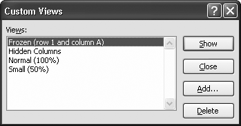
Figure 14-8. You can use this dialog box to show or delete existing views or to create new ones (click Add, and then follow the procedure from step 4, above).
Tip
For some examples of custom views in action, visit this book’s “Missing CD” page at www.missingmanuals.com and download CustomViews.xls, a sample spreadsheet with an array of custom views already set up.
Printing in Excel is pretty straightforward—as long as your spreadsheet fits on a normal 8.5 x 11-inch piece of paper. If you’re one of the millions of spreadsheet owners who don’t belong to that club, welcome to the world of Multiple Page Disorder: the phenomenon in which pages and pages of apparently unrelated and noncontiguous columns start spewing from your printer. Fortunately, Excel comes with a slew of print-tweaking tools designed to help you control what you’re printing. First off, though, it helps to understand the default settings Excel uses when you click the print button.
Note
You can change most of the settings listed; this is just a list of what happens if you don’t adjust any settings before printing a spreadsheet.
In the printout, Excel uses all the formatting characteristics you’ve applied to the cells, including fonts, fills, and borders. However, Excel’s gridlines, row headers, and column headers don’t appear in the printout.
If your data is too long (all the rows won’t fit on one page) or too wide (all the columns won’t fit), Excel prints the data on multiple pages. If your data is both too long and too wide, Excel prints in the following order: all the rows for the first set of columns that fit on a printed page, then all the rows for the next set of columns that fit, and so on (this is known as “down, then over”). When printing on multiple pages, Excel never prints part of an individual column or row.
Excel prints your file in color if you use colors and you’ve got a color printer.
Excel sets margins to 0.75 inches at the top and bottom of the page, and 0.7 inches on the left and right sides of the page. Ordinarily, Excel doesn’t include headers and footers (so you don’t see any page numbers).
Excel doesn’t include hidden rows and columns in the printout.
Printing a worksheet is similar to printing in any other Windows application. Follow these steps:
Choose Office button → Print.
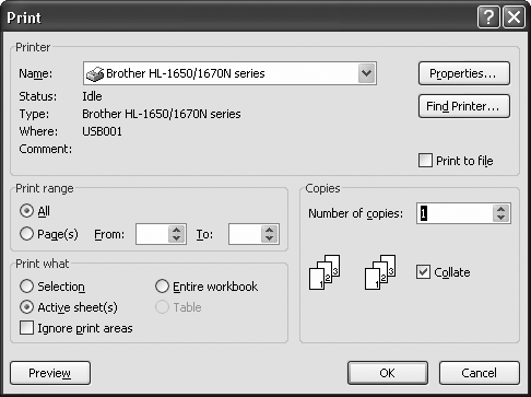
The Print dialog box appears, as shown in Figure 14-9.
Select a printer from the drop-down list.
When the Print dialog box first appears, Excel automatically selects your default printer. If you have more than one printer installed, and you want to use a different printer, then you need to select this printer from the Name pull-down menu. You can also adjust printer settings by clicking the Properties button. Every printer has its own set of options here, but common Properties settings include print quality and paper handling (like double-sided printing for those lucky enough to have a printer that supports it).
Choose what you want to print from the “Print what” box.
The standard option, “Active sheet(s),” prints the current worksheet. If you select “Entire workbook,” Excel prints all the worksheets in your file. Finally, to print out just a portion of a worksheet, select a range of cells, columns, or rows, and then choose Selection.
If you’ve set a print area on your worksheet (see the box on Quick Printing), you can choose “Ignore print areas” to print the full worksheet, not just the print area.
Use the “Print range” box to limit the number of pages that Excel prints.
If you choose All in the “Print range” box, Excel prints as many pages as it needs to output all the data you’ve chosen in the “Print what” box. Alternately, you can choose a range of pages using the Page(s) option. For example, you can choose to print only the first three pages by printing pages from 1 to 3. You can also print just the fourth page by printing from 4 to 4.
Note
In order to use the “Print range” box effectively, you need to know how many pages you need to print your worksheet and what data will appear on each page. Excel’s Page Layout view (Quick Printing), is just the ticket.
Use the “Number of copies” box to print multiple copies of your data.
If you want to print more than one identical copy of your data, change the “Number of copies” text box accordingly. The Collate option determines whether Excel duplicates each page separately. For example, if you print 10 pages and Collate isn’t turned on, Excel prints 10 copies of page 1, 10 copies of page 2, and so on. If Collate is turned on, Excel prints the entire 10-page document, and then prints out another copy, and so on. You’ll still end up with 10 copies of each page, plus, for added convenience, they’ll be grouped together.
Click OK to send the spreadsheet to the printer.
Excel prints your document using the settings you’ve selected.
If you’re printing a very large worksheet, Excel shows a Printing dialog box for a few seconds as it sends the pages to the printer. If you decide to cancel the printing process—and you’re quick enough—you can click the Cancel button in this Printing dialog box to stop the operation. If you don’t possess the cat-like reflexes you once did, you can also open your printer queue to cancel the process. Look for your printer icon in the notification area at the bottom-right of your screen, and double-click that icon to open a print window. Then, select the offending print job in the list, and then press Delete (or choose Document → Cancel from the print window’s menu). Some printers also provide their own cancel button that lets you stop a print job even after it’s left your computer.
If you know that the currently selected printer is the one you want to use, and you don’t want to change any other print settings, you can skip the Print dialog box altogether using the popular (but slightly dangerous) Quick Print feature. Just choose Office button → Print → Quick Print to create an instant printout, with no questions asked.
The Quick Print feature’s so commonly used that many Excel experts add it to the Quick Access toolbar so it’s always on hand. If you want to do this, hover over the Office button → Print → Quick Print command, right-click it, and then choose Add To Quick Access Toolbar. (Appendix A has more about customizing the Quick Access toolbar.)
When you’re preparing to print that 142-page company budget monstrosity, there’s no reason to go in blind. Instead, prudent Excel fans use Page Layout view to check out what their printouts look like before they appear on paper. The tool is especially helpful if you’ve run rampant with formatting, or you want to tweak a variety of page layout settings, and you want to see what the effects will be before clicking Print.
To see the Page Layout view for a worksheet, choose View → Workbook Views → Page Layout View. Or, for an even quicker alternative, use the tiny Page Layout View button in the status bar, which appears immediately to the left of the zoom slider. Either way, you see a nicely formatted preview (Figure 14-10).

Figure 14-10. The Page Layout view shows the first (and part of the second) page of this worksheet’s 76 printed pages. This worksheet has 19 columns, but since they’re wider than the width of a single printed page, the first page includes only the leftmost seven columns, as shown here. You can scroll to the right to see the additional columns that’ll turn up on other pages, or scroll down to see more rows.
How does Page Layout view differ from Normal view? You’ll see several differences, including:
Page Layout view paginates your data. You see exactly what fits on each page, and how many pages your printout requires.
Page Layout view reveals any headers and footers you’ve set as part of the page setup. These details don’t appear in the Normal worksheet view.
Page Layout view shows the margins that Excel will use for your pages.
Page Layout view doesn’t show anything that Excel won’t print (like the letters at the top of each column). The only exception is the cell gridlines, which are shown to help you move around your worksheet.
Page Layout view includes a bit of text in the Status bar that tells you where you are, page-wise, in a large spreadsheet. For example, you might see the text “Page: 5 of 26.”
Note
Don’t confuse Page Layout view with an ordinary print preview. A print preview provides a fixed “snapshot” of your printout. You can look, but you can’t touch. Page Layout view is vastly better because it shows what your printout will look like and it lets you edit data, change margins, set headers and footers, create charts, draw pictures—you get the idea. In fact, you can do everything you do in Normal view mode in Page Layout view. The only difference is you can’t squeeze quite as much data into the view at once.
If you aren’t particularly concerned with your margin settings, you can hide your margins in Page Layout view so you can fit more information into the Excel window. Figure 14-11 shows you how.
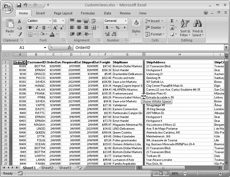
Figure 14-11. Move your mouse between the pages and your mouse pointer changes into this strange two-arrow beast. You can then click to hide the margins in between pages (as shown here),and click again to show them (as shown in Figure 14-10). Either way, you see an exact replica of your printout. The only difference is whether you see the empty margin space.
Here are some of the tasks you may want to perform in Page Layout view:
If the print preview meets with your approval, choose Office button → Print to send the document to the printer.
To tweak print settings and see the effect, choose the Page Layout tab in the ribbon and start experimenting. You’ll learn more about these settings on Excel’s New Features.
To move from page to page, you can use the scroll bar at the side of the window, or you can use the keyboard (like Page Up, Page Down, and the arrow keys). When you reach the edge of your data, you see shaded pages with the text “Click to add data” superimposed. If you want to add information further down the worksheet, just click one of these pages and start typing.
To adjust the page margins, first make sure the ruler is visible by turning on the View → Show/Hide → Ruler checkbox. Then, drag one of the margin lines on the ruler, as shown in Figure 14-12. If you want to set page margins by typing in the exact margin width, use the Page Layout tab of the ribbon instead (Customizing Print Settings).
When you’re ready to return to the Normal worksheet view, choose View → Workbook Views → Normal (or just click the Status bar’s tiny Normal View button).
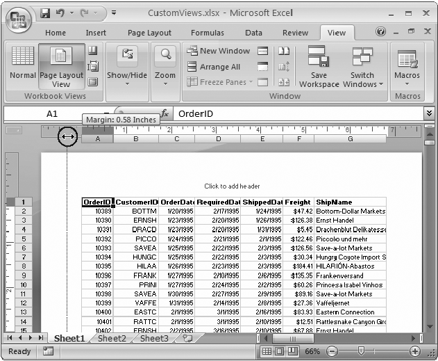
Figure 14-12. The Page Layout view lets you set margins by dragging the margin edge with your mouse. Here, the left margin (circled) is about to be narrowed down to 0.58 inches. If you’re also using a header or footer (below), make sure you don’t drag the page margin above the header or below the footer. If you do, then your header or footer will overlap your worksheet’s data.
A header is a bit of text that’s printed at the top of every page in your printout. A footer is a bit of text that’s printed at the bottom of every page. You can use one, both, or neither in a printout.
Ordinarily, every new workbook starts out without a header or footer. However, Page Layout view gives you an easy way to add either one (or both). Just scroll up to the top of any page to create a header (or the bottom to create a footer), and then look for the box with the text “Click to add header” or “Click to add footer”. Click inside this box, and you can type the header or footer text you want.
Note
You won’t see the header or footer boxes if you’ve drastically compressed your margins. That’s because the header and footer don’t fit. To get them back, resize the margins so that they’re larger. When you’re finished adding the header or footer, you can try adjusting the margins again to see just how small you can get them.
Of course, a good header or footer isn’t just an ordinary piece of text. Instead, it contains information that changes dynamically, like the file name, current page, or the date you printed it. You can get these pieces of information using specialized header and footer codes, which are distinguished by their use of square brackets.
For example, if you enter the code [Page] into a footer, then Excel replaces it with the current page number. If you use the code [Date], then Excel substitutes the current date (when you fire off your printout). Of course, no one wants to memorize a long list of cryptic header and footer codes. To help you get these important details right, Excel adds a new tab to the ribbon named Header & Footer Tools | Design (Figure 14-13) when you edit a header or footer.
The quickest way to get a header or footer is to go to the Header & Footer Tools | Design → Header & Footer section (shown in Figure 14-13), and then choose one of the Header or Footer list’s ready-made options. Some of the options you can use for a header or footer include:
Page numbering (for example, Page 1 or Page 1 of 10)
Worksheet name (for example, Sheet 1)
File name (for example, myfile.xlsx or C:MyDocumentsmyfile.xlsx)
The person who created the document, and the date it was created
A combination of the above information

Figure 14-13. The Header & Footer Tools | Design tab is chock-full of useful ingredients you can add to a header or footer. Click a button in the Header & Footer Elements section to insert a special Excel code that represents a dynamic value, like the current page.
Oddly enough, the header and footer options are the same. It’s up to you to decide whether you want page numbering at the bottom and a title at the top, or vice versa.
If none of the standard options matches what you need, you can edit the automatic header or footer, or you can create your own from scratch. Start typing in the header or footer box, and use the buttons in the Header & Footer Elements section to paste in the code you need for a dynamic value. And if you want to get more creative, switch to the Home tab of the ribbon, and then use the formatting buttons to change the font, size, alignment, and color of your header or footer.
Finally, Excel gives you a few high-powered options in the Header & Footer Tools | Design → Options section. These include:
Different First Page. This option lets you create one header and footer for the first page, and use a different pair for all subsequent pages. Once you’ve checked this option, fill in the first page header and footer on the first page, and then head to the second page to create a new header and footer that Excel can use for all subsequent pages.
Different Odd & Even pages. This option lets you create two different headers (and footers)—one for all even-numbered pages and one for all odd-numbered pages. (If you’re printing a bunch of double-sided pages, you can use this option to make sure the page number appears in the correct corner.) Use the first page to fill in the odd-numbered header and footer, and then use the second page to fill in the even-numbered header and footer.
Scale with Document. If you select this option, then when you change the print scale to fit in more or less information on your printout, Excel adjusts the headers and footers proportionately.
Align with Page Margins. If you select this option, Excel moves the header and footer so that they’re centered in relation to the margins. If you don’t select this option, Excel centers them in relation to the whole page. The only time you’ll notice a difference is if your left and right margins are significantly different sizes.
Excel’s standard print settings are fine if you’ve got a really small amount of data in your worksheet. But most times, you’ll want to tweak these settings so that you can easily read what you print. The Page Layout tab of the ribbon is your control center (Figure 14-14). It lets you do everything from adding headers and footers to shrinking the size of your data so you can cram more information onto a single printed page.
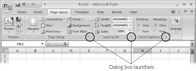
Figure 14-14. The Page Layout tab’s most important print-related sections are Page Setup (which lets you change orientation and margin settings), Scale to Fit (which lets you cram more information into your printed pages), and Sheet Options (which lets you control whether gridlines and column headers appear on the printout). To get even more settings, you can click the dialog box launcher (circled), which pops up a full-fledged Page Setup dialog box.
The Page Layout → Page Setup → Margins list (Figure 14-15) lets you adjust the size of your printed page’s margins (the space between your worksheet data and the edge of the page). All you need to do is pick one of the preset options. The margin numbers indicate the distance between the item indicated (for example, the top of the page, or the footer on the bottom) and the edge of the paper.
Note
The units Excel uses for margins depend on the regional settings on your computer (which you can adjust through the Control Panel’s Regional and Language Options icon). Unfortunately, Excel doesn’t indicate the type of units in the Page Setup dialog box, and it doesn’t give you any choice to override your regional settings and use different units.
Logically enough, when you reduce the size of your margins, you can accommodate more information. However, you can’t completely eliminate your margins. Most printers require at least a little space (usually no less than .25 inches) to grip onto the page, and you won’t be able to print on this part (the very edge of the page). If you try to make the margins too small, Excel won’t inform you of the problem; instead, it’ll just stick with the smallest margin your current printer allows. This behavior is different from that of other Microsoft Office applications (like Word). To see this in action, try setting your margins to 0, and then look at the result in the print preview window. You’ll see there’s still a small margin left between your data and the page borders.
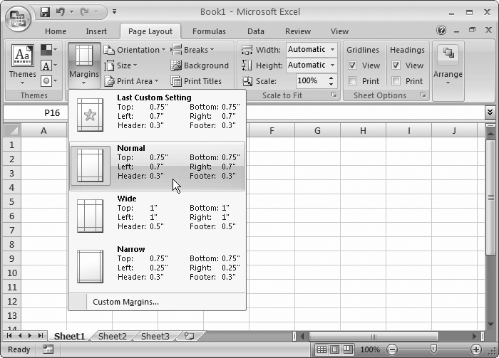
Figure 14-15. You can choose a helpful margin preset (Normal, Wide, or Narrow), or choose Custom Margins to fine-tune your margins precisely, as shown in Figure 14-16.
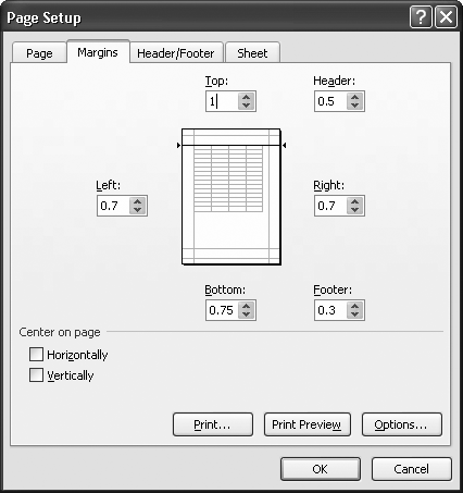
Figure 14-16. Excel allocates space at the top and bottom of your printout for a header or footer. In this example, the header margin is set to 0.5, which means that any header information will appear half an inch below the top of the page. The top margin’s set to 1, meaning the worksheet data will appear one inch below the top of the page. When adjusting either of these settings, be careful to make sure the top margin’s always larger than the header margin; otherwise, your worksheet’s data will print on top of your header.
Tip
A good rule of thumb is to adjust margins symmetrically (printouts tend to look nicest that way). Thus, if you shrink the left margin to 0.5, make the same change to the right margin. Generally, if you want to fit more data and you don’t need any header or footer space, then you can safely reduce all your margins to 0.5. If you really want to cram in the maximum amount of data you can try 0.25, but that’s the minimum margin that most printers allow.
When you have only a few rows or columns of information, you may want to use one of the “Center on page” options at the bottom of the tab. Select Horizontally to center your columns between the left and right margins. Select Vertically to center your data between the top and bottom of the page.
Orientation is the all-time most useful print setting. This setting lets you control whether you’re printing on pages that are upright (in portrait mode) or turned horizontally on their sides (in landscape mode). If Excel is splitting your rows across multiple pages when you print your worksheet, it makes good sense to switch to landscape orientation. That way, Excel prints your columns across a page’s long edge, which accommodates more columns (but fewer rows per page).
If you’re fed up with trying to fit all your data on an ordinary sheet no matter which way you turn it, you may be tempted to try using a longer sheet of paper. You can then tell Excel what paper you’ve decided to use by choosing it from the Paper Size menu. (Of course, the paper needs to fit into your printer.) Letter is the standard 8.5 x 11-inch sheet size, while Legal is another common choice—it’s just as wide but comes in a bit longer at 8.5 x 14 inches.
Margins and orientation are the most commonly adjusted print settings. However, Excel has a small family of additional settings hidden on the Page Setup dialog box’s Sheet tab. To see these, go to the Page Layout → Page Setup section of the ribbon, and click the dialog box launcher (the tiny square-with-an-arrow icon in the bottom-right corner). The Page Setup dialog box appears, as shown in Figure 14-17.
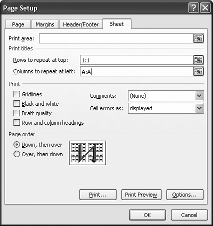
The Sheet tab includes the following settings:
Print area lets you specify the range of cells you want to print. While this tool definitely gets the job done, it’s easier to use the Print Area tool (described in the box on Quick Printing). Some people find the Print dialog box’s Selection setting (How to Print an Excel File) also a more efficient method.
Print titles lets you print specific rows at the top of every page, or specific columns on the left side of every page. For example, you could use this setting to print column titles on the top of every page.
Gridlines prints the grid of lines separating columns and rows that you see on your worksheet.
Figure 14-17. The Page, Margins, and Header/Footer tabs provide options that are easier to configure than using the Page Layout ribbon tab. However, the Sheet tab includes a few options that you can’t find anywhere else. In this example, Excel uses the “Print titles” section to ensure that every page in this printout will display the first row of the spreadsheet as well as the first column.
Row and column headings prints the column headers (which contain the column letters) at the top of each page and the row headers (with the row numbers) on the left side of each page.
Black and white tells Excel to render all colors as a shade of gray, regardless of your printer settings.
Draft quality tells Excel to use lower-quality printer settings to save toner and speed up printing, assuming your printer has these features, of course.
Comments lets you print the comments that you’ve added to a worksheet. Excel can either append them to the cells in the printout or add them at the end of the printout, depending on the option you select.
Cell errors lets you configure how Excel should print a cell if it contains a formula with an error. You can choose to print the error that’s shown (the standard option), or replace the error with a blank value, two dashes (--), or the error code #N/A (meaning not available). You’ll learn much more about formulas in Chapter 15.
Page order sets the way Excel handles a large worksheet that’s too wide and too long for the printed page’s boundaries. When you choose “Down, then over” (the standard option), Excel starts by printing all the rows in the first batch of columns. Once it’s finished this batch, Excel then moves on to the next set of columns, and prints those columns for all the rows in your worksheet, and so on. When you chose “Over, then down,” Excel moves across your worksheet first. That means it prints all the columns in the first set of rows. After it’s printed these pages, it moves to the next set of rows, and so on.
Sooner or later it will happen to you—you’ll face an intimidatingly large worksheet that, when printed, is hacked into dozens of apparently unconnected pages. You could spend a lot of time assembling this jigsaw printout (using a bulletin board and lots of tape), or you could take control of the printing process and tell Excel exactly where to split your data into pages. In the following sections, you’ll learn several techniques to do just that.
One of Excel’s often overlooked but surprisingly handy features is manual page breaks. The idea is you tell Excel explicitly where to start a new page. You can tell Excel to start a new page between subsequent tables on a worksheet (rather than print a page that has the end of the first one and the beginning of the next).
To insert a page break, move to the leftmost column (column A), and then scroll down to the first cell that you want to appear on the new page. Then, choose Page Layout → Page Setup → Breaks → Insert Page Break. You see a dotted line that indicates the dividing lines in between pages (Figure 14-18).
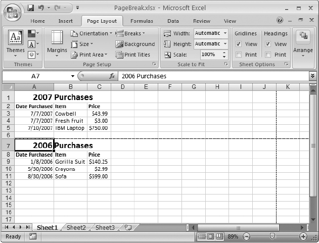
Figure 14-18. Using a page break, you can make sure the second table (“2006 Purchases”) always begins on a new page. The dotted line shows where one page ends and the new page starts. When you add a page break, you see a dotted line for it, and you see a dotted line that shows you where additional page breaks naturally fall, based on your margins, page orientation, and paper size settings.
Tip
There’s no limit to how many page breaks you can add to a worksheet—if you have a dozen tables that appear one after the other, you can place a page break after each one to make sure they all start on a new page.
You can also insert page breaks to split your worksheet vertically into pages. This is useful if your worksheet is too wide to fit on one page, but you want to control exactly where the page break will fall. To do so, move to the first row, scroll to the column where the new page should begin, and then choose Page Layout → Page Setup → Breaks → Insert Page Break.
You can remove page breaks one at a time by moving to an adjacent cell and choosing Page Layout → Page Setup → Breaks → Remove Page Break. Or you can clear them all using Page Layout → Page Setup → Breaks → Reset All Page Breaks.
Page breaks are a nifty feature for making sure your printouts are paginated just the way you want them. However, they can’t help you fit more information on a page. They simply allow you to place page breaks earlier than they would ordinarily occur, so they fall in a more appropriate place.
If you want to fit more on a page, you need to shrink your information down to a smaller size. Excel includes a scaling feature that lets you take this step easily without forcing you to reformat your worksheet.
Scaling lets you fit more rows and columns on a page, by shrinking everything proportionally. For example, if you reduce scaling to 50 percent, you fit twice as many columns and rows on a page. (Keep in mind that the font size in the printout will be smaller, and it may be hard to read.) Conversely, you can use scaling to enlarge your data.
To change the scaling percentage, just type a new percentage into the Page Layout → Scale to Fit → Scale box. The data still appears just as big on your worksheet, but Excel shrinks or expands it in the printout. To gauge the effect, you can use the Page Layout view to preview your printout, as described on Quick Printing.
Rather than fiddling with the scaling percentage (and then seeing what its effect is on your worksheet by trial and error), you may want to force your data to fit into a fixed number of pages. To do this, you set the values in the Page Layout → Scale to Fit → Width box and the Page Layout → Scale to Fit → Height box. Excel performs a few behind-the-scenes calculations and adjusts the scaling percentage accordingly. For example, if you choose one page tall and one page wide, Excel shrinks your entire worksheet so that everything fits into one page. This scaling is tricky to get right (and can lead to hopelessly small text), so make sure you review your worksheet in the Page Layout view before you print it.
You don’t have to be a tree-hugging environmentalist to want to minimize the number of pages you print out. Enter the Page Break Preview, which gives you a bird’s-eye view of how an entire worksheet’s going to print. Page Break Preview is particularly useful if your worksheet is made up of lots of columns. That’s because Page Break Preview zooms out so you can see a large amount of data at once, and it uses thick blue dashed lines to show you where page breaks will occur, as shown in Figure 14-19. In addition, the Page Break Preview numbers every page, placing the label “Page X” (where “X” is the page number) in large gray lettering in the middle of each page.
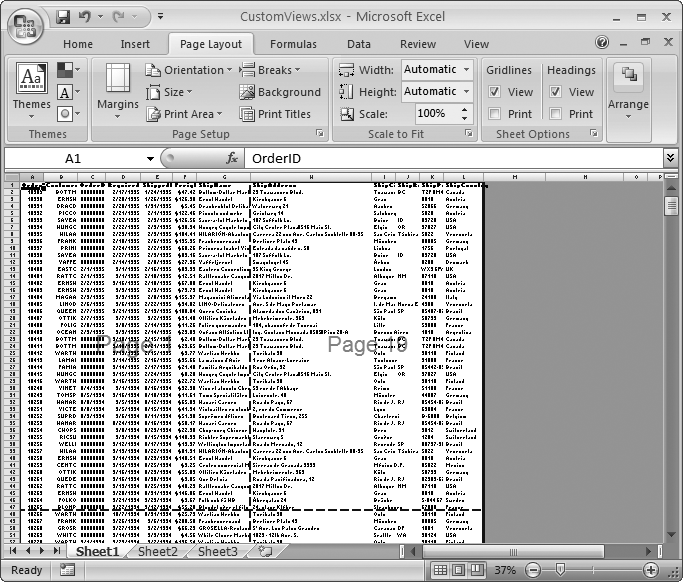
Figure 14-19. This example shows a large worksheet in Page Break Preview mode. The worksheet is too wide to fit on one page (at least in portrait orientation), and the thick dotted line indicates that the page breaks after column G and after row 47. (Excel never breaks a printout in the middle of a column or row.)
To preview the page breaks in your data, select View → Workbook Views → Page Break Preview, or use the tiny Page Break Preview button in the status bar. A window appears, informing you that you can use Page Break Preview mode to move page breaks. You can choose whether you want to see this message again; if not, turn on the “Do not show this dialog again” checkbox before clicking OK.
Once you’re in Page Break Preview mode, you can do all of the things you do in Normal view mode, including editing data, formatting cells, and changing the zoom percentage to reveal more or fewer pages. You can also click the blue dashed lines that represent page breaks, and drag them to include more or less rows and columns in your page.
Excel lets you make two types of changes using page breaks:
You can make less data fit onto a page. To do so, drag the bottom page break up or the left-side page break to the right. Usually, you’ll perform these steps if you notice that a page break occurs in an awkward place, like just before a row with some kind of summary or subtotal.
You can make more data fit onto a page. To do so, drag the bottom page break down or the left-side page break to the left.
Of course, everyone wants to fit more information onto their printouts, but there’s only so much space on the page. So what does Excel do when you expand a page by dragging the page break? It simply adjusts the scaling setting you learned about earlier (on Scaling). The larger you make the page, the smaller the Scaling percentage setting becomes. That means your printed text may end up too tiny for you to read. (The text on your computer’s display doesn’t change, however, so you don’t have any indication of just how small your text has become until you print out your data, or take a look at it in Page Layout view.)
Note
Scaling affects all the pages in your printout. That means when you drag one page break to expand a page, you actually end up compressing all the pages in your workbook. However, the page breaks don’t change for other pages, which means you may end up with empty, unused space on some of the pages.
The best advice: If your goal is merely to fit more information into an entire printout, change the scaling percentage manually (Scaling) instead of using the Page Break Preview. On the other hand, if you need to squeeze just a little bit more data onto a specific page, use the Page Break Preview.