
When you create a basic workbook, you’ve taken only the first step toward mastering Excel. If you plan to print your data, email it to colleagues, or show it off to friends, you need to think about whether you’ve formatted your worksheets in a viewer-friendly way. The careful use of color, shading, borders, and fonts can make the difference between a messy glob of data and a worksheet that’s easy to work with and understand.
But formatting isn’t just about deciding, say, where and how to make your text bold. Excel also lets you control the way numerical values are formatted. In fact, there are really two fundamental aspects of formatting in any worksheet:
Cell appearance. Cell appearance includes cosmetic details like color, typeface, alignment, and borders. When most people think of formatting, they think of cell appearance first.
Cell values. Cell value formatting controls the way Excel displays numbers, dates, and times. For numbers, this includes details like whether to use scientific notation, the number of decimal places displayed, and the use of currency symbols, percent signs, and commas. With dates, cell value formatting determines what parts of the date are shown in the cell, and in what order.
In many ways, cell value formatting is more significant than cell appearance because it can change the meaning of your data. For example, even though 45%, $0.45, and .450 are all the same number, your spreadsheet readers will see a failing test score, a cheap price for chewing gum, and a world-class batting average.
Note
Keep in mind that regardless of how you format your cell values, Excel maintains an unalterable value for every number entered. For more on how Excel internally stores numbers, see the box on Currency.
In this chapter, you’ll learn about cell value formatting, and then unleash your inner artist with cell appearance formatting. You’ll also learn the most helpful ways to use formatting to improve a worksheet’s readability. For information about timesaving features like the Format Painter, styles, and themes, check out Excel 2007: The Missing Manual.
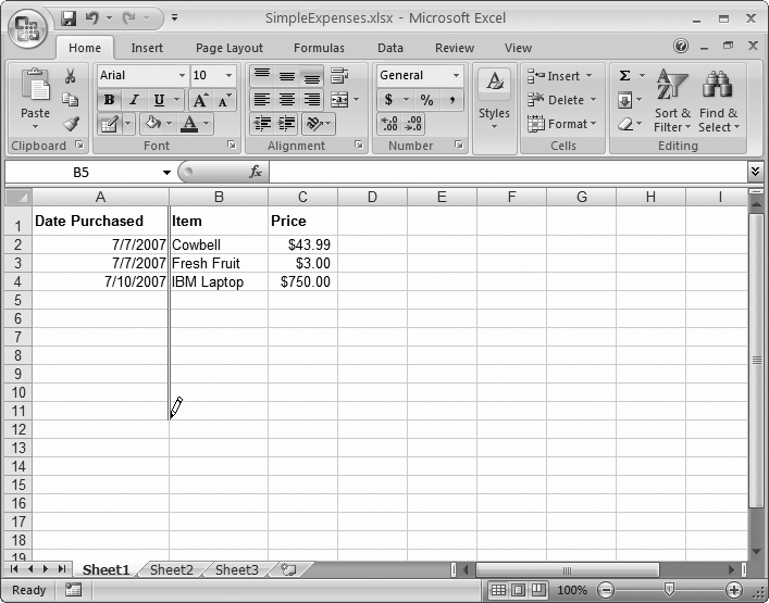
Cell value formatting is one aspect of worksheet design you don’t want to ignore, because the values Excel stores can differ from the numbers that it displays in the worksheet, as shown in Figure 13-1. In many cases, it makes sense to have the numbers that appear in your worksheet differ from Excel’s underlying values, since a worksheet that’s displaying numbers to, say, 13 decimal places, can look pretty cluttered.

Figure 13-1. This worksheet shows how different formatting can affect the appearance of the same data. Each of the cells B2, B3, and B4 contains the exact same number: 5.18518518518519. In the formula bar, Excel always displays the exact number it’s storing, as you see here with cell B2. However, in the worksheet itself, each cell’s appearance differs depending on how you’ve formatted the cell.
To format a cell’s value, follow these steps:
Select the cells you want to format.
You can apply formatting to individual cells or a collection of cells. Usually, you’ll want to format an entire column at once because all the values in a column typically contain the same type of data. Remember, to select a column, you simply need to click the column header (the gray box at the top with the column letter).
Note
Technically, a column contains two types of data: the values you’re storing within the actual cells and the column title in the topmost cell (where the text is). However, you don’t need to worry about unintentionally formatting the column title because Excel applies number formats only to numeric cells (cells that contain dates, times, or numbers). Excel doesn’t use the number format for the column title cell because it contains text.
Select Home → Cells → Format → Format Cells, or just right-click the selection, and then choose Format Cells.
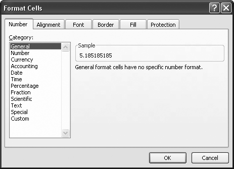
In either case, the Format Cells dialog box appears, as shown in Figure 13-2.
The Number tab’s options let you choose how Excel translates the cell value into a display value. For example, you can change the number of decimal places that Excel uses to show the number. (Number formatting choices are covered in much more detail in the next section, “Formatting Numbers.”)
Most of the Format Cells dialog box’s other tabs are for cell appearance formatting, which is covered later in this chapter.
Note
Once you apply formatting to a cell, it retains that formatting even if you clear the cell’s contents (by selecting it and pressing Delete). In addition, formatting comes along for the ride if you copy a cell, so if you copy the content from cell A1 to cell A2, the formatting comes with it. Formatting includes both cell value formatting and cell appearance.
The only way to remove formatting is to highlight the cell and select Home → Editing → Clear → Clear Formats. This command removes the formatting, restoring the cell to its original, General number format (which you’ll learn more about next), but it doesn’t remove any of the cell’s content.
Click OK.
Excel applies your formatting changes and changes the appearance of the selected cells accordingly.
You’ll spend a lot of time in this chapter at the Format Cells dialog box. As you’ve already seen, the most obvious way to get there is to choose Home → Format → Cells → Format Cells. However, your mouse finger’s sure to tire out with that method. Fortunately, there’s a quicker route—you can use one of three dialog box launchers. Figure 13-3 shows the way.
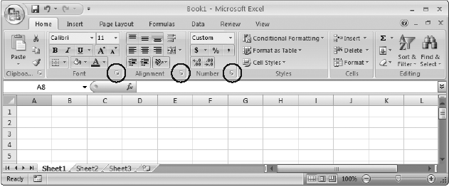
Figure 13-3. The ribbon’s Home tab gives you a quick way to open the Format Cells dialog box from three different spots: the Font, the Alignment, or the Number tab.
In the Format Cells dialog box, the Number tab lets you control how Excel displays numeric data in a cell. Excel gives you a lengthy list of predefined formats (as shown in Figure 13-4). Remember, Excel uses number formats when the cell contains only numeric information. Otherwise, Excel simply ignores the number format. For example, if you enter Half past 12 in a column full of times, Excel considers it plain ol’ text—although, under the hood, the cell’s numerical formatting stays put, and Excel uses it if you change the cell content to a time.
When you create a new spreadsheet, every cell starts out with the same number format: General. This format comes with a couple of basic rules:
If a number has any decimal places, Excel displays them, provided they fit in the column. If the number’s got more decimal places than Excel can display, then it leaves out the ones that don’t fit. (It rounds up the last displayed digit, when appropriate). If you change a column width, then Excel automatically adjusts the amount of digits it displays.
Excel removes leading and trailing zeros. Thus, 004.00 becomes 4. The only exception to this rule occurs with numbers between −1 and 1, which retain the 0 before the decimal point. For example, Excel displays the number .42 as 0.42.
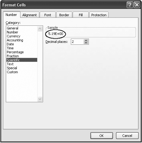
Figure 13-4. You can learn about the different number formats by selecting a cell that already has a number in it, and then choosing a new number format from the Category list (Home → Cells → Format → Format Cells). When you do so, Excel uses the Format Cells dialog box to show how it’ll display the number if you apply that format. In this example, you see that the cell value, 5.18518518518519, will appear as 5.19E+00, which is scientific notation with two decimal places.
As you saw in Chapter 10, the way you type in a number can change a cell’s formatting. For example, if you enter a number with a currency symbol, the number format of the cell changes automatically to Currency. Similarly, if you enter three numbers separated by dashes (-) or backward slashes (/), Excel assumes you’re entering a date, and adjusts the number format to Date.
However, rather than rely on this automatic process, it’s far better just to enter ordinary numbers and set the formatting explicitly for the whole column. This approach prevents you from having different formatting in different cells (which can confuse even the sharpest spreadsheet reader), and it makes sure you get exactly the formatting and precision you want. You can apply formatting to the column before or after you enter the numbers. And it doesn’t matter if a cell is currently empty; Excel still keeps track of the number format you’ve applied.
Different number formats provide different options. For example, if you choose the Currency format, then you can choose from dozens of currency symbols. When you use the Number format, you can choose to add commas (to separate groups of three digits) or parentheses (to indicate negative numbers). Most number formats let you set the number of decimal places.
The following sections give a quick tour of the predefined number formats available in the Format Cells dialog box’s Number tab. Figure 13-5 gives you an overview of how different number formats affect similar numbers.
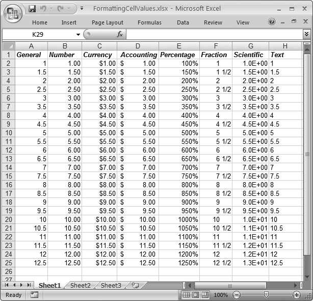
Figure 13-5. Each column contains the same list of numbers. Although this worksheet shows an example for each number format (except dates and times), it doesn’t show all your options. Each number format has its own settings (like the number of decimal places) that affect how Excel displays data.
The General format is Excel’s standard number format; it applies no special formatting other than the basic rules described in the box on Currency. General is the only number format (other than Text) that doesn’t limit your data to a fixed number of decimal places. That means if you want to display numbers that differ wildly in precision (like 0.5, 12.334, and 0.120986398), it makes sense to use General format. On the other hand, if your numbers have a similar degree of precision (for example, if you’re logging the number of miles you run each day), the Number format makes more sense.
The Number format is like the General format but with three refinements. First, it uses a fixed number of decimal places (which you set). That means that the decimal point always lines up (assuming you’ve formatted an entire column). The Number format also allows you to use commas as a separator between groups of three digits, which is handy if you’re working with really long numbers. Finally, you can choose to have negative numbers displayed with the negative sign, in parentheses, or in red lettering.
The Currency format closely matches the Number format, with two differences. First, you can choose a currency symbol (like the dollar sign, pound symbol, Euro symbol, and so on) from an extensive list; Excel displays the currency symbol before the number. Second, the Currency format always includes commas. The Currency format also supports a fixed number of decimal places (chosen by you), and it allows you to customize how negative numbers are displayed.
The Accounting format is modeled on the Currency format. It also allows you to choose a currency symbol, uses commas, and has a fixed number of decimal places. The difference is that the Accounting format uses a slightly different alignment. The currency symbol is always at the far left of the cell (away from the number), and there’s always an extra space that pads the right side of the cell. Also, the Accounting format always shows negative numbers in parentheses, which is an accounting standard. Finally, the number 0 is never shown when using the Accounting format. Instead, a dash (‐) is displayed in its place. There’s really no reason to prefer the Currency or the Accounting format. Think of it as a personal decision, and choose whichever looks nicest on your worksheet. The only exception is if you happen to be an accountant, in which case you really have no choice in the matter—stick with your namesake.
The Percentage format displays fractional numbers as percentages. For example, if you enter 0.5, that translates to 50%. You can choose the number of decimal places to display.
There’s one trick to watch out for with the Percentage format. If you forget to start your number with a decimal, then Excel quietly “corrects” your numbers. For example, if you type 4 into a cell that uses the Percentage format, Excel interprets this as 4%. As a result, it actually stores the value 0.04. A side effect of this quirkiness is that if you want to enter percentages larger than 100%, you can’t enter them as decimals. For example, to enter 200%, you need to type in 200 (not 2.00).
The Fraction format displays your number as a fraction instead of a number with decimal places. The Fraction format doesn’t mean you have to enter the number as a fraction (although you can if you want by using the forward slash, like 3/4). Instead it means that Excel converts any number you enter and display it as a fraction. Thus, to have 1/4 appear you can either enter .25 or 1/4.
Note
If you try to enter 1/4 and you haven’t formatted the cell to use the Fraction number format, then you won’t get the result you want. Excel assumes you’re trying to enter a date (in this case, January 4th of the current year). To avoid this misunderstanding, change the number format before you type in your fraction. Or, enter it as 0 1/4 (zero and one quarter).
People often use the Fraction format for stock market quotes, but it’s also handy for certain types of measurements (like weights and temperatures). When using the Fraction format, Excel does its best to calculate the closest fraction, which depends on a few factors including whether an exact match exists (entering .5 always gets you 1/2, for example) and what type of precision level you’ve picked when selecting the Fraction formatting.
You can choose to have fractions with three digits (for example, 100/200), two digits (10/20), or just one digit (1/2), using the top three choices in the Type list. For example, if you enter the number 0.51, Excel shows it as 1/2 in one-digit mode, and the more precise 51/100 in three-digit mode. In some cases, you may want all numbers to use the same denominator (the bottom number in the fraction) so that it’s easy to compare different numbers. (Don’t you wish Excel had been around when you were in grammar school?) In this case, you can choose to show all fractions as halves (with a denominator of 2), quarters (a denominator of 4), eighths (8), sixteenths (16), tenths (10), and hundredths (100). For example, the number 0.51 would be shown as 2/4 if you chose quarters.
Tip
Entering a fraction in Excel can be awkward because Excel may attempt to convert it to a date. To prevent this confusion, always start by entering 0 and then a space. For example, instead of typing 2/3 enter 0 2/3 (which means zero and two-thirds). If you have a whole number and a fraction, like 1 2/3, you’ll also be able to duck the date confusion.
The Scientific format displays numbers using scientific notation, which is ideal when you need to handle numbers that range widely in size (like 0.0003 and 300) in the same column. Scientific notation displays the first non-zero dirgit of a number, followed by a fixed number of digits, and then indicates what power of 10 that number needs to be multiplied by to generate the original number. For example, 0. 0003 becomes 3.00 x 10⁻⁴ (displayed in Excel as 3.00E-04). The number 300, on the other hand, becomes 3.00 x 10² (displayed in Excel as 3.00E02). Scientists—surprise, surprise—like the Scientific format for doing things like recording experimental data or creating mathematical models to predict when an incoming meteor will graze the Earth.
Few people use the Text format for numbers, but it’s certainly possible to do so. The Text format simply displays a number as though it were text, although you can still perform calculations with it. Excel shows the number exactly as it’s stored internally, positioning it against the left edge of the column. You can get the same effect by placing an apostrophe before the number (although that approach won’t allow you to use the number in calculations).
Excel gives you lots of options here. You can use everything from compact styles like 3/13/07 to longer formats that include the day of the week, like Sunday, March 13, 2007. Time formats give you a similar range of options, including the ability to use a 12-hour or 24-hour clock, show seconds, show fractional seconds, and include the date information.
To format dates and times, first open the Format Cells dialog box shown in Figure 13-7 (Home → Cells → Format → Format Cells). Choose Date or Time from the column on the left and then choose the format from the list on the right. Date and Time both provide a slew of options.
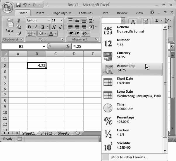
Figure 13-6. The all-around quickest way to apply a number format is to see some cells, and then, from the number format list, choose an option. Best of all, you see a small preview of what the value in the first selected cell will look like if you apply the format.
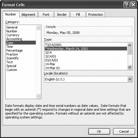
Figure 13-7. Excel gives you dozens of different ways to format that modify the date’s appearance depending on the regional settings of the computer viewing the Excel file, or you can choose a fixed date format. stick to the U.S. standard. Instead, choose the appropriate region from the Locale list box. Each locale provides its own set of customized date formats.
Excel has essentially two types of date and time formats:
Formats that take the regional settings of the spreadsheet viewer’s computer into account. With these formats, dates display differently depending on the computer that’s running Excel. This choice is a good one because it lets everyone see dates in just the way they want to, which means no time-consuming arguments about month-day-year or day-month-year ordering.
Formats that ignore the regional settings of individual computers. These formats define a fixed pattern for month, day, year, and time components, and display date-related information in exactly the same way on all computers. If you need to absolutely make sure a date is in a certain format, use this choice.
The first group (the formats that rely on a computer’s regional settings) is the smallest. It includes two date formats (a compact, number-only format and a long, more descriptive format) and one time format. In the Type list, these formats are at the top and have an asterisk next to them.
The second group (the formats that are independent of a computer’s regional settings) is much more extensive. In order to choose one of these formats, you first select a region from the Locale list, and then you select the appropriate date or time format. Some examples of locales include “English (United States)” and “English (United Kingdom).”
If you enter a date without specifically formatting the cell, Excel usually uses the short region-specific date format. That means that the order of the month and year vary depending on the regional settings of the current computer. If you incorporate the month name (for example, January 1, 2007), instead of the month number (for example, 1/1/2007), Excel uses a medium date format that includes a month abbreviation, like 1-Jan-2007.
Note
You may remember from Chapter 10 that Excel stores a date internally as the cumulative number of days that have elapsed since a certain long-ago date that varies by operating system. You can take a peek at this internal number using the Format Cells dialog box. First, enter your date. Then, format the cell using one of the number formats (like General or Number). The underlying date number appears in your worksheet where the date used to be.
You wouldn’t ever want to perform mathematical operations with some types of numeric information. For example, it’s hard to image a situation where you’d want to add or multiply phone numbers or Social Security numbers.
When entering these types of numbers, therefore, you may choose to format them as plain old text. For example, you could enter the text (555) 123-4567 to represent a phone number. Because of the parentheses and the dash (‐), Excel won’t interpret this information as a number. Alternatively, you could just precede your value with an apostrophe (') to explicitly tell Excel that it should be treated as text (you might do this if you don’t use parentheses or dashes in a phone number).
But whichever solution you choose, you’re potentially creating more work for yourself because you have to enter the parentheses and the dash for each phone number you enter (or the apostrophe). You also increase the likelihood of creating inconsistently formatted numbers, especially if you’re entering a long list of them. For example, some phone numbers may end up entered in slightly similar but somewhat different formats, like 555-123-4567 and (555)1234567.
To avoid these problems, apply Excel’s Special number format (shown in Figure 13-8), which converts numbers into common patterns. And lucky you: In the Special number format, one of the Type options is Phone Number (other formats are for Zip codes and Social Security numbers).
Formatting cell values is important because it helps maintain consistency among your numbers. But to really make your spreadsheet readable, you’re probably going to want to enlist some of Excel’s tools for controlling things like alignment, color, and borders and shading.
To format a cell’s appearance, first select the single cell or group of cells that you want to work with, and then choose Home → Cells → Format → Format Cells, or just right-click the selection, and then choose Format Cells. The Format Cells dialog box that appears is the place where you adjust your settings.

Figure 13-8. Special number formats are ideal for formatting sequences of digits into a common pattern. For example, in the Type list, if you choose Phone Number, then Excel converts the sequence of digits 5551234567 into the proper phone number style—(555) 123-4567—with no extra work required on your part.
Tip
Even a small amount of formatting can make a worksheet easier to interpret by drawing the viewer’s eye to important information. Of course, as with formatting a Word document or designing a Web page, a little goes a long way. Don’t feel the need to bury your worksheet in exotic colors and styles just because you can.
As you learned in the previous chapter, Excel automatically aligns cells according to the type of information you’ve entered. But what if this default alignment isn’t what you want? Fortunately, in the Format Cells dialog box, the Alignment tab lets you easily change alignment as well as control some other interesting settings, like the ability to rotate text.
Excel lets you control the position of content between a cell’s left and right borders, which is known as the horizontal alignment. Excel offers the following choices for horizontal alignment, some of which are shown in Figure 13-9:
General is the standard type of alignment; it aligns cells to the right if they hold numbers or dates and to the left if they hold text. You learned about this type of alignment in Chapter 10.
Left (Indent) tells Excel to always line up content with the left edge of the cell. You can also choose an indent value to add some extra space between the content and the left border.
Center tells Excel to always center content between the left and right edges of the cell.
Right (Indent) tells Excel to always line up content with the right edge of the cell. You can also choose an indent value to add some extra space between the content and the right border.
Fill copies content multiple times across the width of the cell, which is almost never what you want.
Justify is the same as Left if the cell content fits on a single line. When you insert text that spans more than one line, Excel justifies every line except the last one, which means Excel adjusts the space between words to try and ensure that both the right and left edges line up.
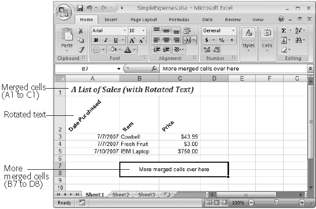
Center Across Selection is a bit of an oddity. When you apply this option to a single cell, it has the same effect as Center. If you select more than one adjacent cell in a row (for example, cell A1, A2, A3), this option centers the value in the first cell so that it appears to be centered over the full width of all cells. However, this happens only as long as the other cells are blank. This setting may confuse you a bit at first because it can lead to cell values being displayed over cells in which they aren’t stored. Another approach to centering large text titles and headings is to use cell merging (as described in the box on Fonts and Color).
Distributed (Indent) is the same as Center—if the cell contains a numeric value or a single word. If you add more than one word, then Excel enlarges the spaces between words so that the text content fills the cell perfectly (from the left edge to the right edge).

Vertical alignment controls the position of content between a cell’s top and bottom border. Vertical alignment becomes important only if you enlarge a row’s height so that it becomes taller than the contents it contains. To change the height of a row, click the bottom edge of the row header (the numbered cell on the left side of the worksheet), and drag it up or down. As you resize the row, the content stays fixed at the bottom. The vertical alignment setting lets you adjust the cell content’s positioning.
Excel gives you the following vertical alignment choices, some of which are shown in Figure 13-9:
Top tells Excel that the first line of text should start at the top of the cell.
Center tells Excel that the block of text should be centered between the top and bottom border of the cell.
Bottom tells Excel that the last line of text should end at the bottom of the cell. If the text doesn’t fill the cell exactly, then Excel adds some padding to the top.
Justify is the same as Top for a single line of text. When you have more than one line of text, Excel increases the spaces between each line so that the text fills the cell completely from the top edge to the bottom edge.
Distributed is the same as Justify for multiple lines of text. If you have a single line of text, this is the same as Center.
If you have a cell containing a large amount of text, you may want to increase the row’s height so you can display multiple lines. Unfortunately, you’ll notice that enlarging a cell doesn’t automatically cause the text to flow into multiple lines and fill the newly available space. But there’s a simple solution: just turn on the “Wrap text” checkbox (on the Alignment tab of the Format Cells dialog box). Now, long passages of text flow across multiple lines. You can use this option in conjunction with the vertical alignment setting to control whether Excel centers a block of text, or lines it up at the bottom or top of the cell. Another option is to explicitly split your text into lines. Whenever you want to insert a line break, just press Alt+Enter, and start typing the new line.
Tip
After you’ve expanded a row, you can shrink it back by double-clicking the bottom edge of the row header. When you haven’t turned on text wrapping, this action shrinks the row back to its standard singleline height.
Finally, the Alignment tab allows you to rotate content in a cell up to 180 degrees, as shown in Figure 13-10. You can set the number of degrees in the Orientation box on the right of the Alignment tab. Rotating cell content automatically changes the size of the cell. Usually, you’ll see it become narrower and taller to accommodate the rotated content.
As in almost any Windows program, you can customize the text in Excel, applying a dazzling assortment of colors and fancy typefaces. You can do everything from enlarging headings to colorizing big numbers. Here are the individual font details you can change:
The font style. (For example, Arial, Times New Roman, or something a little more shocking, like Futura Extra Bold.) Arial is the standard font for new worksheets.
The font size, in points. The default point size is 10, but you can choose anything from a minuscule 1-point to a monstrous 409-point. Excel automatically enlarges the row height to accommodate the font.
Various font attributes, like italics, underlining, and bold. Some fonts have complimentary italic and bold typefaces, while others don’t (in which case Windows uses its own algorithm to make the font bold or italicize it).
The font color. This option controls the color of the text. (Borders and Fills covers how to change the color of the entire cell.)
To change font settings, first highlight the cells you want to format, choose Home → Cells → Format → Format Cells, and then click the Font tab (Figure 13-11).
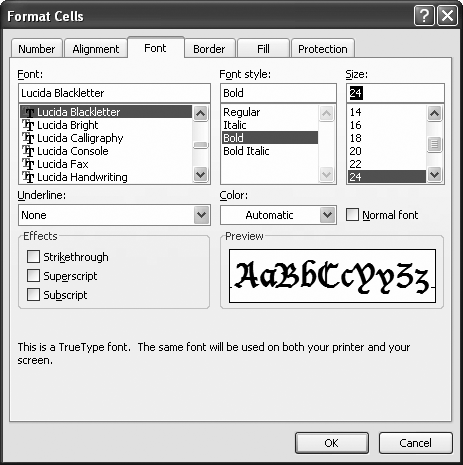
Figure 13-11. Here’s an example of how to apply an exotic font through the Format Cells dialog box. Keep in mind that when displaying data, and especially numbers, sans-serif fonts are usually clearer and look more professional than serif fonts. (Serif fonts have little embellishments, like tiny curls, on the ends of the letters; sans-sarif fonts don’t.) Arial, the default spreadsheet font, is a sans-sarif font.
Tip
Thanks to Excel’s handy Redo feature, you can repeatedly apply a series of formatting changes to different cells. After you make your changes in the Format Cells dialog box, simply select the new cell you want to format in the same way, and then hit Ctrl+Y to repeat the last action.
Rather than heading to the Format Cells dialog box every time you want to tweak a font, you can use the ribbon’s handy shortcuts. The Home → Font section displays buttons for changing the font and font size. You also get a load of tiny buttons for applying basics like bold, italic, and underline, applying borders, and changing the text and background colors. (Truth be told, the formatting toolbar is way more convenient for setting fonts because its drop-down menu shows a long list of font names, whereas the font list in the Format Cells dialog box is limited to showing an impossibly restrictive six fonts at a time. Scrolling through that cramped space is like reading the phone book on index cards.)
Without a doubt, the most useful ribbon formatting feature is Live Preview, a frill that shows you the result of a change before you’ve even applied it. Figure 13-12 shows Live Preview in action.
Note
No matter what font you apply, Excel, thankfully, always displays the cell contents in the formula bar in easy-to-read Calibri font. That makes things easier if you’re working with cells that’ve been formatted using difficult-to-decipher script fonts, or really large or small text sizes.
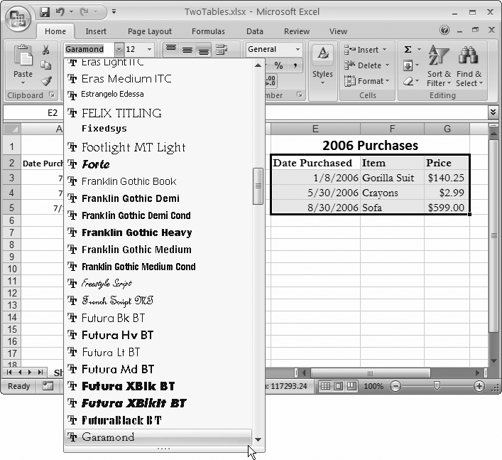
Figure 13-12. Right now, this spreadsheet’s creator is just thinking about using the stylish Garamond font for this table. However, the moment she hovers over Benguiat (higher up in the font list), Excel switches the currently selected cells on the worksheet to that font, providing a preview of the change. The best part: When she moves the mouse pointer away, the formatting disappears instantaneously. To make the changes stick, all she needs to do is click the font. This Live Preview feature works with font names, font sizes, and colors.
Most fonts contain not only digits and the common letters of the alphabet, but also some special symbols that you can type directly on your keyboard. One example is the copyright symbol ©, which you can insert into a cell by entering the text (C), and letting AutoCorrect do its work. Other symbols, however, aren’t as readily available. One example is the special arrow character →. To use this symbol, you’ll need the help of Excel’s symbols. Simply follow these steps:
Choose Insert → Text → Symbol.
The Symbol dialog box opens, as shown in Figure 13-13. Now it’s time to hunt for the symbol you need.
Choose the font and subset (the group of symbols you want to explore).
If you’re looking for a fairly common symbol (like a mathematical sign, an arrow, an accented letter, or a fraction), you probably don’t need to change the font. In the Font box, keep the default selection of “(normal text)”, and then, from the Subset box at the right, choose the type of symbol. For example, choose the Arrows subset to see arrow symbols that point in different directions.
Figure 13-13. The Symbol dialog box lets you insert one or more special characters. You can choose extended characters that are supported by most fonts (like currency symbols, non-English letters, arrows, and so on). Alternatively, you can use a font that’s all about fancy characters, like the Wingdings font that’s chock full of tiny graphical icons.
If you want funkier alternatives, choose a fancy font from the Font box on the left. You should be able to find at least one version of the Wingdings font in the list. Wingdings has the most interesting symbols to use. It’s also the most likely to be on other people’s computers, which makes a difference if you’re planning to email your worksheet to other people. If you get your symbols from a really bizarre font that other people don’t have, they won’t be able to see your symbols.
Note
Wingdings is a special font included with Windows that’s made up entirely of symbols like happy faces and stars, none of which you find in standard fonts. You can try and apply the Wingdings font on your own (by picking it from the font list), but you won’t know which character to press on your keyboard to get the symbol you want. You’re better off using Excel’s Symbol dialog box.
Select the character, and then click Insert.
Alternatively, if you need to insert multiple special characters, just double-click each one; doing so inserts each symbol right next to each other in the same cell without having to close the window.

Tip
If you’re looking for an extremely common special character (like the copyright symbol), you can shorten this whole process. Instead of using the Symbols tab, just click over to the Special Characters tab. Then, look through the small list of commonly used symbols. If you find what you want, just select it, and then click Insert.
There’s one idiosyncrasy that you should be aware of if you choose to insert symbols from another font. For example, if you insert a symbol from the Wingdings font into a cell that already has text, then you actually end up with a cell that has two fonts—one for the symbol character and one that’s used for the rest of your text.
This system works perfectly well, but it can cause some confusion. For example, if you apply a new font to the cell after inserting a special character, Excel adjusts the entire contents of the cell to use the new font, and your symbol changes into the corresponding character in the new font (which usually isn’t what you want). These problems can crop up any time you deal with a cell that has more than one font.
On the other hand, if you kept the font selection on “(normal text)” when you picked your symbol, you won’t see this behavior. That’s because you picked a more commonplace symbol that’s included in the font you’re already using for the cell. In this case, Excel doesn’t need to use two fonts at once.
Note
When you look at the cell contents in the formula bar, you always see the cell data in the standard Calibri font. This consistency means, for example, that a Wingdings symbol doesn’t appear as the icon that shows up in your worksheet. Instead, you see an ordinary letter or some type of extended non-English character, like æ.
The best way to call attention to important information isn’t to change fonts or alignment. Instead, place borders around key cells or groups of cells and use shading to highlight important columns and rows. Excel provides dozens of different ways to outline and highlight any selection of cells.
Once again, the trusty Format Cells dialog box is your control center. Just follow these steps:
Select the cells you want to fill or outline.
Your selected cells appear highlighted.
Select Home → Cells → Format → Format Cells, or just right-click the selection, and then choose Format Cells.
The Format Cells dialog box appears.
Head directly to the Border tab. (If you don’t want to apply any borders, skip straight to step 4.)
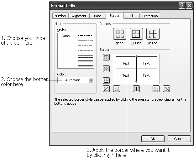
Applying a border is a multistep process (see Figure 13-14). Begin by choosing the line style you want (dotted, dashed, thick, double, and so on), followed by the color. (Automatic picks black.) Both these options are on the left side of the tab. Next, choose where your border lines are going to appear. The Border box (where the word “Text” appears four times) functions as a nifty interactive test canvas that shows you where your lines will appear. Make your selection either by clicking one of the eight Border buttons (which contain a single bold horizontal, vertical, or diagonal line), or click directly inside the Border box. If you change your mind, clicking a border line makes it disappear.
Figure 13-14. Follow the numbered steps in this figure to choose the line style and color, and then apply the border. In this picture, Excel will apply a solid border between the columns and at the top edge of the selection.
For example, if you want to apply a border to the top of your selection, click the top of the Border box. If you want to apply a line between columns inside the selection, click between the cell columns in the Border box. The line appears indicating your choice.
Tip
The Border tab also provides two shortcuts in the tab’s Presets section. If you want to apply a border style around your entire selection, select Outline after choosing your border style and color. Choose Inside to apply the border between the rows and columns of your selection. Choosing None removes all border lines.
Click the Fill tab.
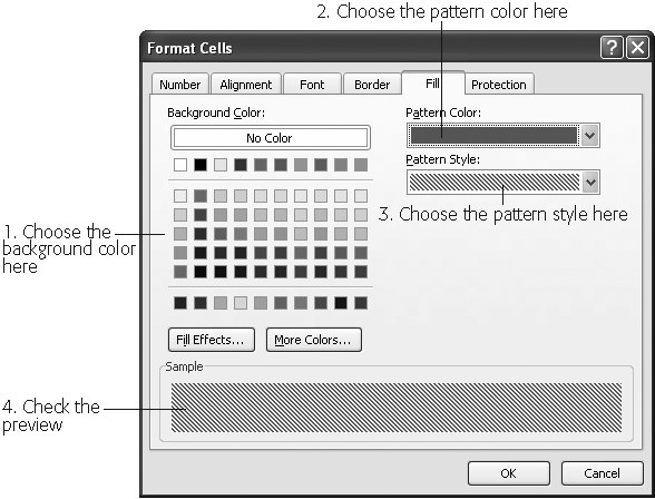
Here you can select the background color, pattern color, and pattern style to apply shading to the cells in the selection (see Figure 13-15). Click the No Color box to clear any current color or pattern in the selected cells.
Note
When picking a pattern color, you may notice that certain colors are described as theme colors. Themes are combinations of coordinated fonts, colors, and effects. For more on themes, check out Excel 2007: The Missing Manual.
To get a really fancy fill, you can use a gradient, which is a blend of two colors. For example, with gradients you can create a fill that starts out white on one side of a cell and gradually darkens to blue on the other. To use a gradient fill, click the Fill Effects button, and then follow the instructions in Figure 13-16.
Figure 13-15. Adding a pattern to selected cells is simpler than choosing borders. All you need to do is select the colors you want and, optionally, choose a pattern. The pattern can include a grid, dots, or the diagonal lines shown in this figure.
Figure 13-16. Top: To create a gradient, you need to pick the two colors that are used to create the blend, and you need to choose the way Excel does the blending (from one side to another, from the top to the bottom, and so on). When applying a gradient fill to a stack of cells, a vertical fill makes the most sense, because that way the gradients in each cell line up and they look like one seamless shaded region. When applying a gradient fill to a row of cells, a horizontal fill looks better for the same reason. Bottom: A gradient fill on cells A2 to A5.
Click OK to apply your changes.
If you don’t like the modifications you’ve just applied, you can roll back time by pressing Ctrl+Z to trigger the indispensable Undo command.

If you need to add a border around a cell or group of cells, the Format Cells dialog box’s Border tab does the trick (see Figure 13-14). However, you could have a hard time getting the result you want, particularly if you want to add a combination of different borders around different cells. In this situation, you have a major project on your hand that requires several trips back to the Format Cells dialog box.
Fortunately, there’s a little-known secret that lets you avoid the hassle: Excel’s Draw Border feature. The Draw Border feature lets you draw border lines directly on your worksheet. This process is a little like working with a painting program. You pick the border style, color, and thickness, and then you drag to draw the line between the appropriate cells. When you draw, Excel applies the formatting settings to each affected cell, just as if you’d used the Borders tab.
Here’s how it works:
Look in the ribbon’s Home → Font section for the border button.
The name of the border button changes to reflect whatever you used it for last. You can most easily find it by its position, as shown in Figure 13-17.
Click the border button, choose Line Style, and then pick the type of line you want.
You can use dashed and solid lines of different thicknesses, just as you can in the Format Cells dialog box’s Borders tab.
Click the border button, choose Line Color, and then pick the color you want.
Now you’re ready to start drawing.
Click the border button, and then choose Draw Border.
When you choose Draw Border, your mouse pointer changes into a pencil icon.
Using the border pencil, click a gridline where you want to place your border (Figure 13-18).
You can also drag side to side or up and down to draw a longer horizontal or vertical line. And if you drag your pointer down and to the side, you create an outside border around a whole block of cells.
To stop drawing, head back to the border menu, and then choose Draw Border again.
If you make a mistake, you can even use an eraser to tidy it all up. Just click the border button, and then choose Erase Border. The mouse pointer changes to an eraser. Now you can click the border you want to remove.

Tip
If you don’t want to use the Draw Border feature, you can still make good use of the border button. Just pick a line style and line color, select some cells, and then choose an option from the border menu. For example, if you pick Bottom Border, Excel applies a border with the color and style you chose to the bottom of the current cell selection.