Now that you’ve created a basic worksheet, and you’re acquainted with Excel and its spiffy new interface, it’s time to get down and dirty adding data. Whether you want to plan your household budget, build a sales invoice, or graph your soaring (or plunging) net worth, you first need to understand how Excel interprets the information you put in your worksheet.
Depending on what kind of data you type into a cell, Excel classifies it as a date, a number, or a piece of text. In this chapter, you’ll learn how Excel makes up its mind, and how you can make sure it makes the right decision. You’ll also learn how to use Excel’s best timesavers, including the indispensable Undo feature.
One of Excel’s most important features is its ability to distinguish between different types of information. A typical worksheet contains both text and numbers. There isn’t a lot you can do in Excel with ordinary text (other than alphabetize a list, perform a simple spell check, and apply some basic formatting). On the other hand, Excel gives you a wide range of options for numeric data. For example, you can string your numbers together into complex calculations and formulas, or you can graph them on a chart. Programs that don’t try to separate text and numbers—like Microsoft Word, for example—can’t provide these features.
Most of the time, when you enter information in Excel, you don’t explicitly indicate the type of data. Instead, Excel examines the information you’ve typed in, and, based on your formatting and other clues, classifies it automatically.
Excel distinguishes between four core data types:
Ordinary text. Column headings, descriptions, and any content that Excel can’t identify as one of the other data types.
Numbers. Prices, integers, fractions, percentages, and every other type of numeric data. Numbers are the basic ingredient of most Excel worksheets.
Dates and times. Dates (like Oct 3, 2007), times (like 4:30 p.m.), and combined date and time information (like Oct 3, 2007, 4:30 p.m.). You can enter date and time information in a variety of formats.
True or false values. This data type (known in geekdom as a Boolean value) can contain one of two things: TRUE or FALSE (displayed in all capitals). You don’t need Boolean data types in most worksheets, but they’re useful for programmer types and power users who want to create complex formulas.
One useful way to tell how Excel is interpreting your data is to look at cell alignment, as explained in Figure 10-1.
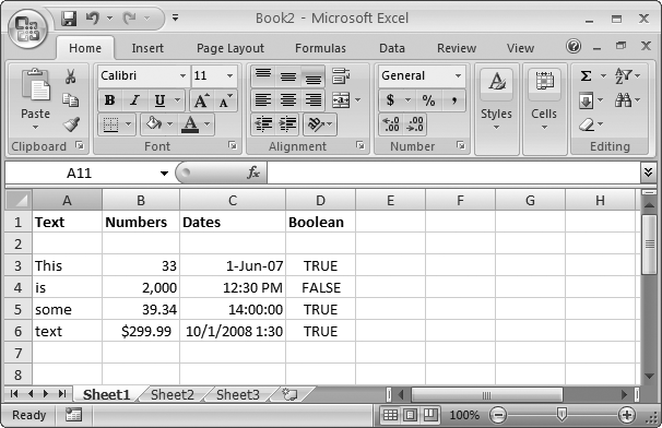
Figure 10-1. Unless you explicitly change the alignment, Excel always left-aligns text (that is, it lines it up against the left edge of a cell), as in column A. On the other hand, it always right-aligns numbers and dates, as in columns B and C. And it centers Boolean values, as in column D.
Note
The standard alignment of text and numbers doesn’t just represent the whims of Excel—it also matches the behavior you want most of the time. For example, when you type in text, you usually want to start at the left edge so that subsequent entries in a column line up. But when entering numbers, you usually want them to line up on the decimal point so that it’s easier to scan a list of numbers and quickly spot small and large values. Of course, if you don’t like Excel’s standard formatting, you’re free to change it, as you’ll see in Chapter 13.
As Figure 10-1 shows, Excel can display numbers and dates in several different ways. For example, some of the numbers include decimal places, one uses a comma, and one has a currency symbol. Similarly, one of the time values uses the 12-hour clock while another uses the 24-hour clock. Other entries include only date information or both date and time information. You might assume that when you type in a number, it will appear in the cell exactly the way you typed it. For example, when you type 3-comma-0-0-0 you expect to see 3,000. However, that doesn’t always happen. To see the problem in action, try typing 3,000 in a cell. It shows up exactly the way you entered it. Then, type over that value with 2000. The new number appears as 2,000. Excel remembers your first entry, and assumes that you want to use thousand separators in this cell all the time.
These differences may seem like a spreadsheet free-for-all, but don’t despair—you can easily set the formatting of numbers and dates. (In fact, that’s the subject of Chapter 13.) At this point, all you need to know is that the values Excel stores in each cell don’t need to match exactly the values that it displays in each cell. For example, the number 4300 could be formatted as plain old 4300 or as the dollar amount $4,300. Excel lets you format your numbers so you have exactly the representation you want. At the same time, Excel treats all numbers equivalently, no matter how they’re formatted, which lets you combine them together in calculations. Figure 10-2 shows you how to find the underlying stored value of a cell.
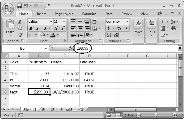
Figure 10-2. You can see the underlying value that Excel is storing for a cell by selecting the cell and then glancing at the formula bar. In this sheet, you can see that the value $299.99 is actually stored without the dollar currency symbol, which Excel applied only as part of the display format. Similarly, Excel stores the number 2,000 without the comma; it stores the date 1-Jun-07 as 6/1/2007; the time 12:30 p.m. as 12:30:00 PM, and the time 14:00:00 as 2:00:00 PM.
Note
Excel assigns data types to each cell in your worksheet, and you can’t mix more than one data type in the same cell. For example, when you type in 44 fat cats, Excel interprets the whole thing as text because it contains letters. If you want to treat 44 as a number (so that you can perform calculations with it, say), then you need to split this content into two cells—one that contains the number 44 and one that contains the remaining text.
By looking at cell alignment, you can easily tell how Excel is interpreting your data. That’s helpful. But what happens when Excel’s interpretation is at odds with your wishes? For example, what if you type in something you consider a number but Excel freakishly treats it as text, or vice versa? The first step to solving this problem is grasping the logic behind Excel’s automatic decision-making process.
If your cell meets any of the following criteria, Excel automatically treats the content as ordinary text:
It contains any letters. Thus, C123 is text, not a number.
It contains any punctuation that Excel can’t interpret numerically. Punctuation allowed in numbers and dates includes the comma (,), the decimal point (.), and the forward slash (/) or dash (‐) for dates. When you type in any other punctuation, Excel treats the cell as text. Thus, 14! is text, not a number.
Occasionally, Excel reads your data the wrong way. For example, you may have a value—like a social security number or a credit card number—that’s made up entirely of numeric characters but that you want to treat like text because you don’t ever want to perform calculations with it. But Excel doesn’t know what you’re up to, and so it automatically treats the value as a number. You can also run into problems when you precede text with the equal sign (which tells Excel that you have a formula in progress), or when you use a series of numbers and dashes that you don’t intend to be part of a date (for example, you want to enter 1-2-3 but you don’t want Excel to read it as January 2, 2003—which is what it wants to do).
In all these cases, the solution’s simple. Before you type the cell value, start by typing an apostrophe ('). The apostrophe tells Excel to treat the cell content as text. Figure 10-3 shows you how it works.

Figure 10-3. To have Excel treat any number, date, or time as text, just precede the value with an apostrophe (you can see the apostrophe in the formula bar, but not in the cell). This worksheet shows the result of typing 1-2-3, both with and without the initial apostrophe.
When you precede a numeric value with an apostrophe, Excel checks out the cell to see what’s going on. When Excel determines that it can represent the content as a number, it places a green triangle in the top left corner of the cell and gives you a few options for dealing with the cell, as shown in Figure 10-4.

Figure 10-4. In this worksheet, the number 42 is stored as text, thanks to the apostrophe that precedes it. Excel notices the apostrophe, wonders if it’s an unintentional error, and flags the cell by putting a tiny green triangle in the top-left corner. If you move to the cell, an exclamation mark icon appears, and, if you click that, a menu appears, letting you choose to convert the number or ignore the issue for this cell.
Note
When you type in either false or true (using any capitalization you like), Excel automatically recognizes the data type as Boolean value instead of text, converts it to the uppercase word FALSE or TRUE, and centers it in the cell. If you want to make a cell that contains false or true as text and not as Boolean data, start by typing an apostrophe (') at the beginning of the cell.
Excel automatically interprets any cell that contains only numeric characters as a number. In addition, you can add the following non-numeric characters to a number without causing a problem:
One decimal point (but not two). For example, 42.1 is a number, but 42.1.1 is text.
One or more commas, provided you use them to separate groups of three numbers (like thousands, millions, and so on). Thus 1,200,200 is a valid number, but 1,200,20 is text.
A currency sign ($ for U.S. dollars), provided it’s at the beginning of the number.
A percent symbol at the beginning or end of the number (but not both).
A plus (+) or minus (−) sign before the number. You can also create a negative number by putting it in parentheses. In other words, entering (33) is the same as entering –33.
An equal sign at the start of the cell.
The most important thing to understand about entering numbers is that when you choose to add other details like commas or the dollar sign, you’re actually doing two things at once: you’re entering a value for the cell and you’re setting the format for the cell, which affects how Excel displays the cell. Chapter 13 provides more information about number styles and shows how you can completely control cell formatting.
When typing in a date, you have a choice of formats. You can type in a full date (like July 4, 2007) or you can type in an abbreviated date using dashes or slashes (like 7-4-2007 or 7/4/2007), which is generally easier. If you enter some numbers formatted as a date, but the date you entered doesn’t exist (like the 30th day in February or the 13th month), then Excel interprets it as text. Figure 10-5 shows you the options.
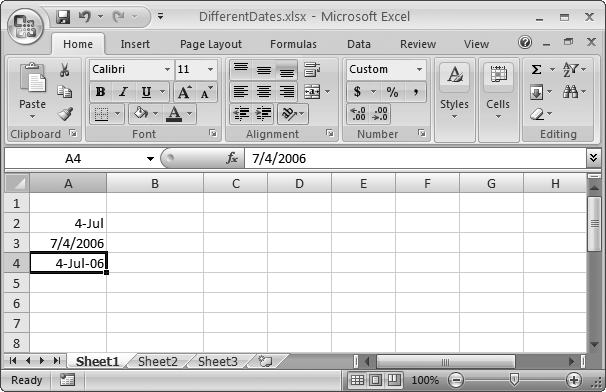
Figure 10-5. Whichever way you type in the date in a cell, it always appears the same on the formula bar (the specific formula bar display depends on the regional settings on your computer, explained next).
Because you can represent dates a few different ways, working with them can be tricky, and you’re likely to encounter some unexpected behavior from Excel. Here are some tips for using dates, trouble-free:
Instead of using a number for the month, you can use a three-letter month abbreviation, but you must put the month in the middle. In other words, you can use 7/4/2007 and 4/Jul/2007 interchangeably.
When you use a two-digit year as part of a date, Excel tries to guess whether the first two digits of the year should be 20 or 19. When the two-digit year is from 00 to 29, Excel assumes it belongs to the 21st century. If the year is from 30 to 99, Excel plants it in the 1900s. In other words, Excel translates 7/4/29 into 7/4/2029, while 7/4/30 becomes 7/4/1930.
Tip
If you’re a mere mortal and you forget where the cutoff point is, enter the year as a four-digit number, which prevents any confusion.
If you don’t type in any year at all, Excel automatically assumes you mean the current year. For example, when you enter 7/4, Excel inserts the date 7/4/2007 (assuming it’s currently 2007 on your computer’s internal clock). When you enter a date this way, the year component doesn’t show up in the cell, but it’s still stored in the worksheet (and visible on the formula bar).
Excel understands and displays dates differently depending on the regional settings on your computer. Windows has a setting that determines how your computer interprets dates (see the box on How Excel decides your data is a date or time). On the U.S. system, Month-Day-Year is the standard progression. But on the UK system, Day-Month-Year is the deal. For example, in the U.S., either 11-7-08 or 11/7/08 is shorthand for November 7, 2008. In the UK, the same notations refer to July 11, 2008.
Thus, if your computer has U.S. regional settings turned on, and you type in 11/7/08, then Excel understands it as November 7, 2008, and the formula bar displays 11/7/08.
Note
The way Excel recognizes and displays dates varies according to the regional settings on your computer, but the way Excel stores dates does not. This feature comes in handy when you save a work-sheet on one computer and then open it on another computer with different regional settings. Because Excel stores every date the same way, the date information remains accurate on the new computer, and Excel can display it according to the new regional settings.
Typing in times is more straightforward than typing in dates. You simply use numbers, separated by a colon (:). You need to include an hour and minute component at minimum (as in 7:30), but you can also add seconds, milliseconds, and more (as in 7:30:10.10). You can use values from 1 to 24 for the hour part, though if your system is set to use a 12-hour clock, Excel converts the time accordingly (in other words, 19:30 becomes 7:30 PM). If you want to use the 12-hour clock when you type in a time, follow your time with a space and the letters P or PM (or A or AM).
Finally, you can create cells that have both date and time information. To do so, just type the date portion first, followed by a space, and then the time portion. For example, Excel happily accepts this combo: 7/4/2008 1:30 PM.
Behind the scenes, Excel stores dates as serial numbers. It considers the date January 1, 1900 to be day 1. January 2, 1900 is day 2, and so on, up through the year 9999. This system is quite nifty because if you use Excel to subtract one date from another, then you actually end up calculating the difference in days, which is exactly what you want. On the other hand, it means you can’t enter a date in Excel that’s earlier than January 1, 1900 (if you do, Excel treats your date like text).
Similarly, Excel stores times as fractional numbers from 0 to 1. The number 0 represents 12:00 a.m. (the start of the day) and 0.999 represents 11:59:59 p.m. (the end of the day). As with dates, this system allows you to subtract one time value from another.

Some of Excel’s timesaving frills can make your life easier when you’re entering data in a worksheet. This section covers four such features: AutoComplete, AutoCorrect, AutoFill, and AutoFit, along with Excel’s top candidates for the Lifetime Most Useful Achievement award: Undo and Redo.
Note
Excel really has two types of automatic features. First off, there are features that do things to your spreadsheets automatically, namely AutoComplete and AutoCorrect. Sometimes that’s cool and convenient, but other times it can send you running for the old manual typewriter. Fortunately, you can turn off both. Excel also has “auto” features that really aren’t that automatic. These include AutoFill and AutoFit, which never run on their own.
Some worksheets require that you type in the same information row after row. For example, if you’re creating a table to track the value of all your Sesame Street collectibles, you can type in Kermit only so many times before you start turning green. Excel tries to help you out with its AutoComplete feature, which examines what you type, compares it against previous entries in the same column, and, if it recognizes the beginning of an existing word, fills it in.
For instance, in your Sesame Street worksheet, if you already have Kermit in the Characters column, when you start typing a new entry in that column beginning with the letter K, Excel automatically fills in the whole word Kermit. Excel then selects the letters that it’s added (in this case, ermit). You now have two options:
If you want to accept the AutoComplete text, move to another cell. For example, when you hit the right arrow key or press Enter to move down, Excel leaves the word Kermit behind.
If you want to blow off Excel’s suggestion, just keep typing. Because Excel automatically selects the AutoComplete portion of the word (ermit), your next keystrokes overtype that text. Or, if you find the AutoComplete text is distracting, then press Delete to remove it right away.
Tip
When you want to use the AutoComplete text but change it slightly, turn on edit mode for the cell by pressing F2. Once you enter edit mode, you can use the arrow keys to move through the cell and make modifications. Press Enter or F2 to switch out of edit mode when you’re finished.
AutoComplete has a few limitations. It works only with text entries, ignoring numbers and dates. It also doesn’t pay any attention to the entries you’ve placed in other columns. And finally, it takes a stab at providing you with a suggestion only if the text you’ve typed in matches another column entry unambiguously.
This means that when your column contains two words that start with K, like Kermit and kerplop, Excel doesn’t make any suggestion when you type K into a new cell, because it can’t tell which option is the most similar. But when you type Kerm, Excel realizes that kerplop isn’t a candidate, and it supplies the AutoComplete suggestion Kermit.
If you find AutoComplete annoying, you can get it out of your face with a mere click of the mouse. Just select Office button → Excel Options, choose the Advanced section, and look under the “Editing options” heading for the “Enable AutoComplete for cell values” setting. Turn this setting off to banish AutoComplete from your spreadsheet.
As you type text in a cell, AutoCorrect cleans up behind you—correcting things like wrongly capitalized letters and common misspellings. AutoCorrect is subtle enough that you may not even realize it’s monitoring your every move. To get a taste of its magic, look for behaviors like these:
If you type HEllo, AutoCorrect changes it to Hello.
If you type friday, AutoCorrect changes it to Friday.
If you start a sentence with a lowercase letter, AutoCorrect uppercases it.
If you scramble the letters of a common word (for example, typing thsi instead of this, or teh instead of the), AutoCorrect replaces the word with the proper spelling.
If you accidentally hit Caps Lock key, and then type jOHN sMITH when you really wanted to type John Smith, Excel not only fixes the mistake, it also switches off the Caps Lock key.
Note
AutoCorrect doesn’t correct most misspelled words, just common typos. To correct other mistakes, use the spell checker described on Spell Check.
For the most part, AutoCorrect is harmless and even occasionally useful, as it can spare you from delivering minor typos in a major report. But if you need to type irregularly capitalized words, or if you have a garden-variety desire to rebel against standard English, then you can turn off some or all of the AutoCorrect actions.
To reach the AutoCorrect settings, select Office button → Excel Options. Choose the Proofing section, and then click the AutoCorrect Options button. (All AutoCorrect options are language specific, and the title of the dialog box that opens indicates the language you’re currently using.) Most of the actions are self-explanatory, and you can turn them off by turning off their checkboxes. Figure 10-7 explains the “Replace text as you type” option, which isn’t just for errors.

Figure 10-7. Under “Replace text as you type” is a long list of symbols and commonly misspelled words (the column on the left) that Excel automatically replaces with something else (the column on the right). But what if you want the copyright symbol to appear as a C in parentheses? You can remove individual corrections (select one, and then click Delete); or you can change the replacement text. And you can add your own rules. For example, you might want to be able to type PESDS and have Excel insert Patented Electronic Seltzer Delivery System. Simply type in the “Replace” and “With” text, as shown here, and then click OK.
Tip
For really advanced AutoCorrect settings, you can use the Exceptions button to define cases where Excel won’t use AutoCorrect. When you click this button, the AutoCorrect Exceptions dialog box appears with a list of exceptions. For example, this list includes abbreviations that include the period but shouldn’t be capitalized (like pp.) and words where mixed capitalization is allowed (like WordPerfect).
AutoFill is a quirky yet useful feature that lets you create a whole column or row of values based on just one or two cells that Excel can extrapolate into a series. Put another way, AutoFill looks at the cells you’ve already filled in a column or row, and then makes a reasonable guess about the additional cells you’ll want to add. People commonly use AutoFill for sequential numbers, months, or days.
Here are a few examples of lists that AutoFill can and can’t work with:
The series 1, 2, 3, 4 is easy for Excel to interpret—it’s a list of steadily increasing numbers. The series 5, 10, 15 (numbers increasing by five) is just as easy. Both of these are great AutoFill candidates.
The series of part numbers CMP-40-0001, CMP-40-0002, CMP-40-0003 may seem more complicated because it mingles text and numbers. But clever Excel can spot the pattern easily.
Excel readily recognizes series of months (January, February, March) and days (Sun, Mon, Tue), either written out or abbreviated.
A list of numbers like 47, 345, 6 doesn’t seem to follow a regular pattern. But by doing some analysis, Excel can guess at a relationship and generate more numbers that fit the pattern. There’s a good chance, however, that these won’t be the numbers you want, so take a close look at whatever Excel adds in cases like these.
Bottom line: AutoFill is a great tool for generating simple lists. When you’re working with a complex sequence of values, it’s no help—unless you’re willing to create a custom list (Filtering with the List of Values) that spells it out for Excel.
Tip
AutoFill doubles as a quick way to copy a cell value multiple times. For example, if you select a cell in which you’ve typed Cookie Monster, you can use the AutoFill technique described below to fill every cell in that row or column with the same text.
To use AutoFill, follow these steps:
Fill in a couple of cells in a row or column to start off the series.
Technically, you can use AutoFill if you fill in only one cell, although this approach gives Excel more room to make a mistake if you’re trying to generate a series. Of course, when you want to copy only a single cell several times, one cell is a sufficient start.
Select the cells you’ve entered so far. Then click (and hold) the small black square at the bottom-right corner of the selected box.
You can tell that your mouse is in the correct place when the mouse pointer changes to a plus symbol (+).
Drag the border down (if you’re filling a column of items) or to the right (if you’re filling a row of items).
As you drag, a tooltip appears, showing the text that Excel is generating for each cell.
While you’re dragging, you can hold down Ctrl to affect the way that Excel fills a list. When you’ve already filled in at least two cells, Ctrl tells Excel to just copy the list multiple times, rather than look for a pattern. When you want to expand a range based on just one cell, Ctrl does the opposite: It tells Excel to try to predict a pattern, rather than just copy it.
When you release the mouse, Excel automatically fills in the additional cells, and a special AutoFill icon appears next to the last cell in the series, as shown in Figure 10-8.
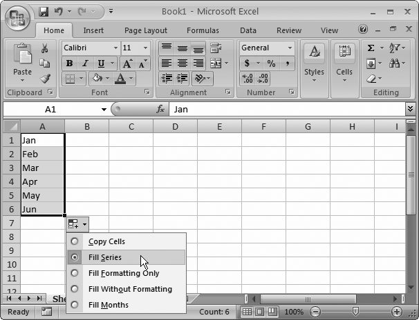
Figure 10-8. After AutoFill does its magic, Excel displays a menu that lets you fill the series without copying the formatting, or copy the formatting without filling the series. You can also choose to copy values instead of generating a list. For example, if you choose to copy values—or Copy Cells, as Excel calls it—then in the two-item series Jan, Feb, you end up with Jan, Feb, Jan, Feb, rather than Jan, Feb, Mar, Apr.
Excel stores a collection of AutoFill lists that it refers to every time you use the feature. You can add your own lists to the collection, which extends the series AutoFill recognizes. For example, Excel doesn’t come set to understand Kermit, Cookie Monster, Grover, Big Bird, Oscar, and Snuffleupagus as a series, but you can add it to the mix.
But why bother to add custom lists to Excel’s collection? After all, if you need to type in the whole list before you use it, is AutoFill really saving you any work? The benefit occurs when you need to create the same list in multiple worksheets, in which case you can type it in just once and then use AutoFill to recreate it as often as you’d like.
To create a custom list, follow these steps:
Choose Office button → Excel Options.
The familiar Excel Options window appears.
Choose the Popular section, and then click Edit Custom Lists.
Here, you can take a gander at Excel’s predefined lists, and add your own (Figure 10-9).
In the “Custom lists” box on the left side of the dialog box, select NEW LIST.
This action tells Excel that you’re ready to create a new list.
In the “List entries” box on the right side of the dialog box, type in your list.
Separate each item with a comma or by pressing Enter. The list in Figure 10-9 shows a series of color names separated by commas.
If you’ve already typed your list into your worksheet, you can save some work. Instead of retyping the list, click inside the text box labeled “Import list from cells.” Then, click the worksheet and drag to select the cells that contain the list. (Each item in the list must be in a separate cell, and the whole list should be in a series of adjacent cells in a single column or a single row.) When you’re finished, click Import, and Excel copies the cell entries into the new list you’re creating.
Click Add to store your list.
At any later point in time, you can return to this dialog box, select the saved list, and modify it in the window on the right. Just click Add to commit your changes after making a change, or click Delete to remove the list entirely.
Click OK to close the Custom Lists dialog box, and OK again to close the Excel Options window.
You can now start using the list with the current worksheet or in a new work-sheet. Just type the first item in your list and then follow the AutoFill steps outlined in the previous section.

Adding Data (Figure 9-7) explained how you can drag the edge of a column to resize it. For greater convenience, Excel also provides an AutoFit feature that automatically enlarges columns to fit overflowing contents perfectly (unfortunately, it doesn’t include a shrink-to-fit option).
The AutoFit feature springs into action in three situations:
When you type a number or date that’s too wide to fit into a cell, Excel automatically widens the column to accommodate the new content. (Excel doesn’t automatically expand columns when you type in text, however.)
If you double-click the right edge of a column header, Excel automatically expands the column to fit the widest entry it contains. This trick works for all types of data, including dates, numbers, and text.
If you select Home → Cells → Format → AutoFit Selection, Excel automatically expands the column to fit the content in the active cell. This feature is helpful if you have a column that’s made up of relatively narrow entries, but which also has a long column title. In this situation, you may not want to expand the column to the full width of the title. Instead, you may wish to size the column to fit a typical entry and allow the title to spill over to the next column.
While AutoFit automatically widens columns when you type in a number or date in a cell, you can still shrink a column after you’ve entered your information.
Keep in mind, however, that when your columns are too narrow, Excel displays the cell data differently, depending on the type of information. When your cells contain text, it’s entirely possible for one cell to overlap (and thereby obscure) another, a problem first described in Chapter 9. However, if Excel allowed truncated numbers, it could be deceiving. For example, if you squash a cell with the price of espresso makers so that they appear to cost $2 (instead of $200), you might wind up ordering a costly gift for all your coworkers. To prevent this problem, Excel never truncates a number or date. Instead, if you’ve shrunk a cell’s width so that the number can’t fit, then you’ll see a series of number signs (like #####) filling in the whole cell. This warning is just Excel’s way of telling you that you’re out of space. Once you enlarge the column by hand (or by using AutoFit), the original number reappears. (Until then, you can still see the number stored in the cell by moving to the cell and looking in the formula bar.)
While editing a worksheet, an Excel guru can make as many (or more) mistakes as a novice. These mistakes include copying cells to the wrong place, deleting something important, or just making a mess of the cell formatting. Excel masters can recover much more quickly, however, because they rely on Undo and Redo. Get in the habit of calling on these features, and you’ll be well on your way to Excel gurudom.Undo and
How do they work? As you create your worksheet, Excel records every change you make. Because the modern computer has vast resources of extra memory and computing power (that is, when it’s not running the latest three-dimensional real-time action game), Excel can keep this log without slowing your computer down one bit.
If you make a change to your worksheet that you don’t like (say you inadvertently delete your company’s entire payroll plan), you can use Excel’s Undo history to reverse the change. In the Quick Access toolbar, simply click the Undo button (Figure 10-10), or press the super-useful keyboard shortcut Ctrl+Z. Excel immediately restores your worksheet to its state just before the last change. If you change your mind again, you can revert to the changed state (known to experts as “undoing your undo”) by choosing Edit → Redo, or pressing Ctrl+Y.
Things get interesting when you want to go farther back than just one previous change, because Excel doesn’t just store one change in memory. Instead, it tracks the last 100 actions you made. And it tracks just about anything you do to a worksheet, including cell edits, cell formatting, cut and paste operations, and much more. As a result, if you make a series of changes you don’t like, or if you discover a mistake a little later down the road, then you can step back through the entire series of changes, one at a time. Every time you press Ctrl+Z, you go back one change in the history. This ability to reverse multiple changes makes Undo one of the most valuable features ever added to any software package.

Figure 10-10. Top: When you hover over the Undo button, you see a text description for the most recent action, which is what you’ll undo if you click away. Here, the text Hello has just been typed into a cell, as Excel explains. Bottom: Click the down-pointing arrow on the edge of the Undo button to see a history of all your recent actions, from most recent (top) to oldest (bottom). If you click an item that’s down the list, you’ll perform a mega-undo operation that undoes all the selected actions. In this example, three actions are about to be rolled back—the text entry in cell B2, and two format operations (which changed the number format and the background fill of cell A2).
Tip
The Undo feature means you don’t need to be afraid of performing a change that may not be what you want. Excel experts often try out new actions, and then simply reverse them if the actions don’t have the desired effect.
The Undo feature raises an interesting dilemma. When you can go back 100 levels into the history of your document, how do you know exactly what changes you’re reversing? Most people don’t remember the previous 100 changes they made to a worksheet, which makes it all too easy to reverse a change you actually want to keep. Excel provides the solution by not only keeping track of old worksheet versions, but also by keeping a simple description of each change. You don’t see this description if you use the Ctrl+Z and Ctrl+Y shortcuts. However, when you hover over the button in the Quick Access toolbar, you’ll see the action you’re undoing listed there.
For example, if you type hello into cell A1, and then delete it, when you hover over the Undo button in the Quick Access toolbar, it says “Undo Clear (Ctrl+Z)”. When you choose this option, the word hello returns. And if you hover over the Undo button again, it now says, “Undo Typing ‘hello’ in A2 (Ctrl+Z)”, as shown in Figure 10-10, top.
Note
Occasionally, when you perform an advanced analysis task with an extremely complex worksheet, Excel may decide it can’t afford to keep an old version of your worksheet in memory. When Excel hits this point, it warns you before you make the change, and gives you the chance to either cancel the edit or continue (without the possibility of undoing the change). In this rare situation, you may want to cancel the change, save your worksheet as a backup, and then continue.