11

IONOSPHERIC PROPAGATION

11.1 INTRODUCTION¹

The nature of the interaction of electromagnetic waves with the ionosphere depends strongly on the frequency of operation. Therefore, the choice of the most convenient model of the resulting propagation phenomena also depends on the frequency.

In the VLF band, for example, the most convenient way to describe the propagation is by means of the so-called “spherical waveguide” mode. This formalism has the ionosphere (modeled as a magnetic conductor) acting as the upper boundary and the Earth surface (modeled as an electric conductor) acting as the bottom boundary of an effective curved “waveguide”. This formalism is particularly convenient at VLF because the transverse dimensions of the effective waveguide are of the same order of magnitude as the wavelength of operation, which means that the propagation can be well described using a few low-order modes. Ionospheric VLF signals can be reasonably stable, but two major obstacles exist in this frequency band. First, such low frequencies require large antennas with high transmit powers. Second, the information (or bit) transmission rates achieved are relatively low because of the low carrier frequency. Despite these disadvantages, ionospheric VLF propagation has been used in applications related to long-distance communications, navigation, and standard frequency dissemination. With the advent of communication satellites, long-distance fiber-optic systems, and global navigation satellite systems such as GPS, the relative importance of VLF/LF ionospheric links for communications and navigation has diminished considerably. An important exception is submarine communications, which still routinely rely on VLF transmitters.²

The waveguide mode formalism can also be used in the LF band, but the computations become more cumbersome due to the larger number of modes necessary for an adequate description of field behaviors. The LF band can be considered as a transition region, and above 100 kHz the skywave mode of operation discussed below for the MF and HF bands is more applicable [1,2].

Under suitable conditions, electromagnetic waves in the MF and HF bands launched from the Earth may be refracted by the ionosphere and returned to the Earth at long distances away from the transmitter. For this “skywave” mode, the small wavelengths compared to the physical scales involved make a ray description more convenient. In many ways, this mode is similar to tropospheric ducting, except that the “reflection” occurs in the stratosphere. As a result, transcontinental distances can be spanned by relatively low-powered transmissions using modest equipment. Such ionospheric links are more suited to MF and HF frequencies because—as we will see later in this chapter—at the VHF band and above the waves penetrate fully through the ionosphere and fail to return back to Earth. Before the advent of satellite communications, MF and HF ionospheric links were the principal means of transcontinental communications. Even though their relative importance has diminished, MF and HF ionospheric links are still an important tool for applications such as “shortwave” broadcasting (especially for less developed countries), amateur radio links (ham radio), diplomatic and military communications, and aid agencies. Because of the relatively modest equipment required, ionospheric skywave links also provide a robust backup mode of long-range communications if fiber-optic or space-based communications infrastructure is disrupted.

Some peculiar effects are observed in ionospheric skywave links. Broadband signals can suffer a great deal of distortion, and therefore these links are most frequently used for narrowband signals, although broadband transmission is possible if distortion is compensated. Even with voice transmissions, the received voice quality may vary considerably over a period of a few seconds as the condition of the ionosphere changes. Ionospheric disturbances may at times create problems with communications in these frequency bands, especially in polar regions, for periods ranging from hours to days.

In this chapter, we will first focus on understanding MF and HF ionospheric links. Later in the chapter, we will also consider the effect of the ionosphere as a source of perturbations on higher frequency Earth–space links traversing the ionosphere, that is, on trans-ionospheric links.

To understand how MF and HF ionospheric links behave, one must first examine how waves travel in an ionized medium and obtain expressions for the refractive index of such a medium. This can then be combined with knowledge of the ionosphere's properties to predict the behavior of MF and HF ionospheric links. Since the magnetic field of the Earth is relatively weak, it is useful to consider first the case of an ionized medium without an externally applied magnetic field before proceeding to the more general, but more complicated, case of a magnetoionic medium.

FIGURE 11.1 Electron motion in an applied field.

11.2 DIELECTRIC PROPERTIES OF AN IONIZED MEDIUM

When an electric field is applied in a medium with free charges, the charges (free electrons, positive ions, and/or negative ions) are accelerated. Because the ions have much greater mass than the electrons, ionic motions are relatively small and can be ignored for most purposes. We shall neglect them here.

Let the displacement of an electron due to the applied electric field be denoted as , as illustrated in Figure 11.1. The result is the same as if the electron had remained where it was and a dipole had been added as shown in Figure 11.2. The dipole moment induced by the electric field due to the motion of the electron is , where e = 1.602 × 10⁻¹⁹ C is the electron charge magnitude. If there are N free electrons per unit volume and the average electron displacement is , the volume polarization that results is

Recall now that it is precisely such volume polarization due to induced dipole moments that determines the behavior of dielectrics. The equation of motion of an electron can be used to find the polarization. An electron in the presence of an electric field will experience a force , causing the electron to accelerate parallel to the electric field (note forces on the electron due to the magnetic field associated with are much smaller and can be neglected). The electron position is therefore written as

FIGURE 11.2 Representation as dipole moment.

where the electric field direction is taken as . In addition to the accelerating force of the electric field, the electron can also experience a frictional force resulting from the effects of collisions with neutral molecules. Now from the equation of motion , with the acceleration, we have

where m_e is the electron mass (9.109 × 10⁻³¹ kg), and the parameter ν is called the electron collision frequency (this name should not be interpreted too literally).

Now consider a time-harmonic electric field

The resulting electron displacement will also be time harmonic:

Recall for an arbitrary phasor that

so that differentiation with respect to time is equivalent to multiplying by jω. The phasor equivalent of equation (11.3) is therefore

or

Substituting this into the phasor equivalents of (11.1) and (11.2)

gives

This can be simplified by defining the angular plasma frequency ω_N (rad/s) as

with N in electrons per cubic meter (so that Hz), and the dimensionless constants

and

to give

For isotropic dielectrics, one can define a relative dielectric constant (which as in Chapter 9 denotes ∈^e/∈₀) through

with real for lossless media, but complex for lossy media. The relative dielectric constant determines the propagation constant of a plane wave in the medium since

where is the refractive index. In the case of complex n², the root should be chosen so that exponentially decaying fields (due to losses) ensue.

From equations (11.15) and (11.16) follows

In the absence of collisions, Z = 0, and we can simplify the formula for the relative permittivity to

with N again in electrons per cubic meter in the final two forms.

Figure 11.3 plots equation (11.19) versus frequency with the electron number density as a parameter. From (11.19) and Figure 11.3, it is evident that the relative permittivity is negative when the frequency of the wave is less than the plasma frequency of the medium. According to (11.18), this results in an imaginary refractive index. This means that any wave transmitted into such a medium will be attenuated exponentially, without any phase change, and will become negligible in a relatively short distance. On the other hand, (11.19) and Figure 11.3 show that the relative permittivity approaches unity if the frequency of the wave is much greater than the plasma frequency. Then the refractive index approaches that of free space, and the wave is less strongly affected by the ionized medium. This is why VHF and higher frequency signals travel through the ionosphere instead of being reflected. Some effects remain even at VHF and higher frequencies, as discussed later in this chapter in connection with Earth–satellite communication and navigation systems. Also, the influence of the ionosphere increases (i.e., the relative permittivity is more different from unity) as the electron number density is increased.

FIGURE 11.3 Relative permittivity versus frequency for a lossless, nonmagnetized ionosphere. Electron density N in inverse cubic meters is indicated in legend, along with the associated plasma frequency f_N.

11.3 PROPAGATION IN A MAGNETOIONIC MEDIUM

In the presence of a static magnetic field , electrons moving at velocity experience a force proportional to . The magnitude of this force is zero when the electron moves parallel to and maximum when it moves transversely with respect to . Such a medium has a built-in directionality, which characterizes an anisotropic medium.

Are plane waves still possible solutions of Maxwell's equations in such a medium? If so, under what condition? What is the impedance they see, and what is their propagation constant (or, equivalently, the refractive index)? We shall answer these questions by writing Maxwell's equations and the equation of motion for free electrons in the medium. The divergence equations are automatically satisfied for a plane wave that has and perpendicular to the propagation direction. This leaves three vector equations: the two curl equations and one equation of motion. Taking one component at a time, this gives nine linear scalar equations in the nine scalar variables that are the components of . From there on it is a matter of algebraic manipulation to eliminate variables, and this can be done in a variety of ways. Along the way one finds, first, that the characteristic impedance is given by . Then one finds that the equations are consistent (i.e., have a solution) only for two specific values of the polarization ratio R, and these depend both on the medium parameters and on the direction of propagation. This means that the medium will allow propagation of plane waves only for particular polarizations specified by the medium. These are known as characteristic polarizations. Finally, an explicit formula for the refractive index for each characteristically polarized wave is obtained. This formula is known by a variety of names, but most often it is called the Appleton or Appleton–Hartree equation.

11.3.1 Mathematical Derivation of the Appleton–Hartree Equation

Assume that the plane wave can exist and that it propagates in the z direction. Then, by the properties of a plane wave, the z dependence is given by and there is no x or y dependence. From Maxwell's equations, we have

Taking the x component of the above

Since there is no y dependence, ∂/∂y ≡ 0 for any field polarization component. Since the z dependence for all quantities is , we have

Treating the other two components similarly gives

and

Similarly, from

one gets

Equations (11.23) and (11.27) show that there is no longitudinal component of , , and , but (11.23) does not guarantee . The plane wave will be transverse only with respect to the , , and vectors, which differs from the isotropic case.

From (11.25) and (11.26) follows

Thus, the characteristic impedance is given by , just as for an isotropic medium. If (11.26) is solved for and the result is used in (11.21), one obtains

.

Hence, the square of the refractive index is given by

Similarly, if (11.25) is solved for and the result used in (11.22), one obtains

Equations (11.29) or (11.30) can be used to find n² if the ratios and are known. For a meaningful solution they must be equal, so that (11.29) and (11.30) give the same result, requiring

from which we can obtain

where R is the polarization ratio of the wave.

Up to this point, we have considered only Maxwell's equations for a plane wave propagating in the z direction in a generalized medium. To determine the ratios , , which we need to solve (11.29) or (11.30) for n², we write the equation of motion of an “average” electron, since it is the displacement of electrons due to that causes the polarization . The equation of motion is

where the second term on the left-hand side again represents the viscous or frictional effects of collisions. The electric and magnetic field forces on the electron are represented on the right-hand side, and represents the Earth's static magnetic field intensity (amplitudes of typically range from 30 to 60 μT). In order to be complete, (11.33) should also include another term corresponding to the force produced by the (time-varying) magnetic field of the wave. However, the magnetic field magnitude of the wave turns out to be negligible compared to the magnitude of the Earth's magnetic field, and hence that term is ignored here.

FIGURE 11.4 Definition of y axis.

It is now necessary to be more specific with respect to the coordinate system. So far we have required the z axis to be in the propagation direction but left the x and y axes arbitrary. Let us now fix the y axis by noting that the propagation direction (z axis) and the vector together define a plane. Let the y axis lie in this plane as shown in Figure 11.4.

In the figure, we have drawn the y axis so that the angle θ, between the propagation direction and the Earth's magnetic field, is acute. This is not necessary, and y could have been directed downward as well, making θ obtuse. In either case, the x axis must be taken to satisfy a right-handed coordinate system. The longitudinal component of is defined as H_0z = H₀ cos θ ≡ H_L and the transverse component as H_0y = H₀ sin θ ≡ H_T.

Note that this choice of coordinates in no way restricts the generality of the derivation. This is true because no matter what the propagation direction may be, we can always take the z axis parallel to it, and no matter what the direction may be (as long as it is not in the z direction), we can always take the y axis so that lies in the yz plane. Then, we can choose the x axis to complete a right-handed orthogonal coordinate system. Clearly, this is a recipe for any combination of propagation direction and magnetic field direction as long as they are not parallel. If they are parallel, any choice of y and x axes that results in a right-handed coordinate system is acceptable.

With this coordinate system established, the equation of motion (11.33) can now be broken into three scalar equations. Starting with the x component, one gets

Since the system is linear, a sinusoidal field

will result in sinusoidal displacements and (11.34) can be replaced by its phasor counterpart

The polarization is produced by the electron displacements via

and therefore

We can substitute these relationships back into (11.35) to get

Multiplication by ∈₀/e gives

To simplify this equation, note that ∈₀m_e/Ne² has dimension (sec)² and μ₀eH_L/m_e has dimension (sec)⁻¹. As in the isotropic plasma case, we define the plasma frequency ω_N by

and additionally define two new quantities, the longitudinal and transverse gyrofrequencies, ω_L and ω_T, respectively, as

Note that the magnitudes of these quantities are the angular frequencies at which an electron traveling in a direction perpendicular to the respective magnetic field component would complete a circular orbit, hence the name. Equation (11.41) now becomes

Finally, substituting the dimensionless quantities

and multiplying through by X gives

The reason for the lengthy algebra discussed previously now becomes apparent: we have now an equation involving only the and components needed for finding n² and dimensionless constants X, Y_L, Y_T, and Z that specify the medium properties and the Earth's magnetic field.

Going back to the y and z components of the equation of motion (11.33) and treating them in the same way gives

The objective is now to eliminate variables to calculate n² by equations (11.29) or (11.30). Let us arbitrarily choose (11.30) so that we wish to retain , and eliminate , , , and . Equation (11.23) has not been used so far and therefore is available. Equations (11.21) and (11.26) as well as (11.22) and (11.25) were used before to eliminate components, but they were redundant as shown by (11.29) and (11.30). The redundancy resulted in (11.32), which is therefore independent and available.

Solving (11.23) for gives

which can be used to eliminate from (11.52) to give

Solving for and substituting the result in (11.50) eliminates and gives, with the use of (11.32),

This equation has in each term on the right and on the left. Hence, it can be solved for the desired ratio, but it is not the only such equation! Using (11.32) to eliminate from (11.51) and multiplying by R gives

Clearly, the solution for will be acceptable only if it satisfies both (11.55) and (11.56). Noting the left-hand sides are the same for these two, one can equate the right-hand sides to obtain

Recall that X, Y_L, Y_T, and Z depend only on the properties of the plasma and the magnetic field , fixed by the physical scenario. Thus (11.57) must be considered a condition on R. Solving the quadratic equation gives

The meaning of this equation is that only plane waves with these two characteristic polarization states are able to retain their polarization state as the wave propagates through the medium.

If (11.58) is satisfied, that is, when the polarizations are characteristic of the medium, (11.55) and (11.56) give the same value for ,

which can then be used in (11.30) to give

in which R must have the characteristic values given by (11.58). When these are substituted in (11.60), one finally obtains the Appleton–Hartree formula

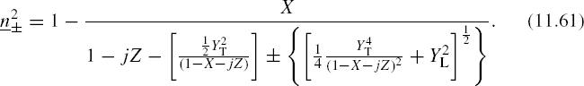
Note that the refractive index calculated with the top sign of (11.61) goes with the polarization given by the top sign in (11.58).

11.3.2 Physical Interpretation

In general, with an anisotropic medium, such as the ionosphere in the Earth's magnetic field, there are two modes of plane wave propagation. Each of these has a particular polarization that depends entirely on the properties of the ionosphere and magnetic field and that can be calculated by (11.58) when these quantities are known. Each of these modes has a particular phase velocity and attenuation constant that can be calculated from the refractive index (the square root of (11.61)). If losses are present (ν and therefore Z are not zero), the square of the refractive index will be complex, otherwise it will be real. The two modes travel at different phase velocities. Hence, they are refracted differently and travel different paths, and when both are present, they do not stay in phase from place to place. In other words, they do not add constructively (in phase) at every point. A wave that does not have one of these characteristic polarizations does not retain its polarization state as it traverses the medium.

In describing propagation through the ionosphere, it is often possible to neglect the Earth's magnetic field and treat the ionosphere as isotropic. When this is not possible, one has to determine the characteristic modes (polarizations) by (11.58), express the incident field in terms of these modes, trace each one separately through the ionosphere, and then recombine them as they exit the ionosphere.

The Appleton–Hartree formula, (11.61), is quite useful for numerical calculations. However, it is too messy for most analytical developments. In the developments to follow, some simplifications will be made. For example, in calculating losses due to absorption the magnetic field may play a rather minor role and may often be neglected. Furthermore, absorption may be unimportant in determining the path of a ray. When such approximations are made, the results will not be precise, but nevertheless suggestive of what happens in the real ionosphere.

11.3.3 Ordinary and Extraordinary Waves

In many cases (i.e., various X, Y_L, Y_T, and Z values), including those most commonly encountered in the ionosphere, one of the solutions is not too different from that with no static magnetic field . This solution is called the ordinary (o-)wave. The other is called the extraordinary (x-)wave. “Extraordinary” here does not mean unusual, and both waves are usually present.

When the characteristic polarization ratios or refractive indices are computed directly from (11.58) and (11.61), the solution using, say, the top sign in (11.58) and (11.61) may correspond to the ordinary wave for 0 < X < 1 and abruptly jump to the extraordinary wave for X > 1. The converse is then true for the other sign. Together, they always give both waves. This odd behavior is simply due to the behavior of the complex square root, which is a two-valued function. Most computers choose the principal root for the complex square root function, regardless of the physics of the situation.

The behavior of the refractive index as a function of frequency is often presented using graphs of , or of the pairs n_R and n_I or and . Plots of , or versus frequency are called dispersion curves.³ It is also common in the ionospheric literature to plot these quantities as a function of instead of ω. When this is done, it is important to recognize that larger X values can correspond either to lower frequencies or to larger electron densities. Figure 11.5 provides example plots of n² versus X for Z = 0, θ = 45° (so that ), and for Y = 1/2 (Figure 11.5a) and 2 (Figure 11.5b). The nonmagnetic curve is also included and is seen to be most similar to the ordinary wave, while the extraordinary wave exhibits larger variations, including, in some cases, behaviors reminiscent of resonant systems.

FIGURE 11.5 Sample dispersion curves for θ = 45°, Z = 0, and (a) Y = 0.5 and (b) Y = 2. The case with Y = 0 is also included for comparison; note Y_L = Y cos θ and Y_T = Y sin θ.

For the lossless case, the ordinary wave can always be identified as the one that passes through the point (X, n²) = (1, 0). When loss is large, the dispersion curves may have little resemblance to the lossless case, and direct identification of the two waves can be difficult. In principle, the ordinary wave can always be identified as that for which the dispersion curves deform continuously so as to pass through the point (X, n²) = (1, 0) as Z is gradually reduced to zero.

11.3.4 The Q_L and Q_T Approximations

When propagation is parallel to the Earth's magnetic field (Y_T = 0), the characteristic polarizations are found from (11.58) to be circular, R = ±j. This condition is called longitudinal propagation. For propagation perpendicular to the Earth's magnetic field (Y_L = 0), the characteristic polarizations are linear, R = 0 and R = ∞. This condition is called transverse propagation. In both cases, the expression (11.61) for the refractive indices greatly simplifies. For these approximations to be useful, Y_T and Y_L need not vanish completely. It is only necessary that the terms in which they appear, respectively, become negligible. These conditions are known as quasi-longitudinal (Q_L) and quasi-transverse (Q_T) propagation. In particular, the Q_L approximation is often very useful, and it can be valid for a surprisingly large range of angles. A frequently used simplification of (11.61) for the lossless Q_L case is

which is valid for , and the + applies to the ordinary wave. For a 10 MHz wave in a plasma having ω_N = 3 × 10⁷ rad/s and gyrofrequency μ₀eH₀/m_e = 8 × 10⁶ rad/s, for example, this condition is satisfied for angles as large as θ = 50°. In this situation, the characteristic polarizations of the wave can still be described adequately as quasi-circular.

Under Q_L conditions, an incoming linearly polarized wave will be subject to a progressive change in the direction of polarization. This occurs because a linearly polarized wave can always be decomposed into left- and right-circular polarized waves propagating along the same direction, as seen in Chapter 3. These two circularly polarized waves, which are the characteristic waves of the medium, have different phase velocities. As a result, their relative phase angle at any given point along the direction of propagation gradually changes as the wave propagates. This causes the direction of the resulting linearly polarized wave, which is the superposition of the characteristic waves, to rotate as it progresses in space. This phenomenon is called Faraday rotation, and it is particularly relevant for satellite communication links, for example, because it can cause severe cross-polarization interference in dual-polarized systems that rely on linear polarized antennas. For this reason, circular polarized systems are more commonly used for satellite transmissions in regions where ionospheric Faraday rotation occurs. In such systems, left- and right-circular polarized waves can carry different signals with little mutual interference when the Q_L condition is satisfied. Additional discussion of Faraday rotation effects is provided later in this chapter.

11.4 IONOSPHERIC PROPAGATION CHARACTERISTICS

Ionospheric links over long distances have some unusual properties. One is the existence of a maximum usable frequency (MUF): for a given propagation path as the carrier frequency is increased, eventually a frequency is reached above which the signal disappears quite abruptly. Another is the skip distance: for a given frequency the signal may be received over a wide range of distances, but there exists a minimum distance for the signal to be received at that frequency. The signal seems to “skip” over the shorter distances and can be received only further away. A third characteristic is selective fading: even for narrowband modulation, some sidebands fade while others are enhanced in a pattern that changes continuously in time. Consequently, analog voice communications often have a strange tonal quality. To understand these qualities of ionospheric propagation, we need to lay some groundwork. The approach will be the superposition of two sets of curves. One is the “ionogram” that gives information about the pertinent ionospheric conditions. The other is a set of “transmission curves” that are based on Snell's law for the particular path. Together, they give information about the propagation possibilities for a particular path under given ionospheric conditions. The development of these concepts is rather long, but important because of the physical insights it provides. Your patience is requested!

11.5 IONOSPHERIC SOUNDING

Although Chapman's theory discussed in the previous chapter provides some idea of the behavior of ionized layers, especially the E and F₁ regions, it is not sufficiently accurate to describe these layers for propagation predictions, and it fails completely when the F₂ region is involved. Ionospheric sounding is an observational tool to provide information about local properties of the ionosphere. Historically, the conventional form of ionospheric sounding has been through the use of ground-based frequency-swept pulsed radars (Figure 11.6).

Most ground-based ionospheric sounders (ionosondes) direct their beams vertically upward and are denoted as vertical sounders. Only ground-based vertical sounders will be considered in any detail here, although oblique sounders can also be used. In the former case, the receiving system is collocated with the transmitting system (monostatic radar). Ground-based ionosondes are also called “bottom-side” sounders, as they collect data from the lower regions of the ionosphere, up to the F region electron density maximum. “Topside” sounders, on the other hand, are space-based sounders that collect data from the top portions of the ionosphere.

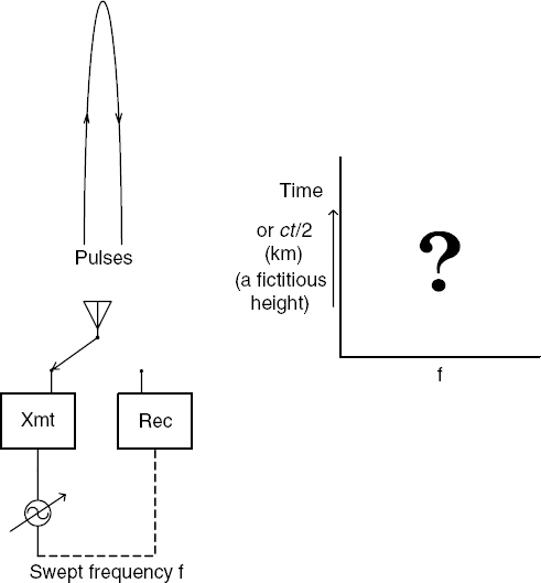
FIGURE 11.6 Ionospheric sounder.

A ground-based ionosonde transmits pulsed signals up to the ionosphere and records properties of the pulses that reflect and return to the ground. The center frequency of these pulses is changed in time, usually in small increments from pulse to pulse, and the time delay between the transmission of each pulse and its reception after reflection from the ionosphere is recorded as a function of frequency. The resulting time versus frequency record is called an ionogram. Ionospheric sounders are very important in ionospheric research in general, and they are also important for understanding the peculiarities of ionospheric propagation. While the vertical axis of an ionogram really represents time, it is customary to multiply this time by c/2, where c is the speed of light in vacuum, and label the vertical scale as a height. As will be seen in what follows, the waves do not actually travel at the velocity c, and the height of reflection in an ionogram is therefore called the virtual height, generally denoted h′, to distinguish it from the true maximum height h of an actual ray path.

11.5.1 Ionograms

To determine how an ionogram might look, the conditions for “reflection” in the ionosphere and the time required to get to the reflection point and back need to be examined.

Snell's law requires, for an oblique path in a horizontally stratified medium, that

where θ(h) is the angle of the ray with respect to the vertical and θ_I is the corresponding incidence angle at the entrance of the ray into the ionosphere. For simplicity, it is assumed that n = n_R = 1 just below the ionosphere. At the maximum height of penetration, θ = 90°, so

For vertical incidence sounding, we have

We therefore need to look at the conditions that force the real part of the refractive index, n_R, to vanish. Consider the lossless case, where Z = 0. For the o-wave, (11.61) becomes

While it is not at all obvious, for n = 0 the solution is X = 1, as can be shown by expanding the square root with the binomial theorem and taking the limit as X → 1. The o-wave will therefore be reflected from the height at which X = 1 (where ω = ω_N). For the x-wave, there are two solutions for n− = 0: X = 1 − Y and X = 1 + Y, where (also not obvious). The extraordinary rays are therefore reflected at heights where the electron density is such that X = 1 − Y or X = 1 + Y. For a wave coming from the ground, the electron density, ω_N, and therefore X will initially be an increasing function of height, and the height for which X = 1 − Y will be reached first. This is therefore the usual reflection height for the extraordinary wave. Under certain conditions, by a complex process called mode coupling, part of the x-wave may leak through the X = 1 − Y region and propagate further upward, to be reflected at the height where the electron density satisfies the X = 1 + Y condition. The wave then returns to the ground by the inverse process. Such a wave is sometimes called a z-wave although it is really just an x-wave arriving back at the ground by a rather complicated process.

To return to the question about what is the actual shape of an ionogram, it is now necessary to look at the velocity of propagation of the waves, since the ionogram actually represents the time for the wave to travel up to the reflection region and back down. Since the travel time of pulses is being considered, an understanding of the group velocity υ_g will be needed. The following discussion will be restricted to the lossless, isotropic case, but still captures the dominant physical properties for more general cases.

It is convenient to define first a group velocity refractive index, n_g, for a lossless, isotropic ionosphere. From n = k₁/k₀ = k₁c/ω and υ_p = ω/k₁ follows

which shows how n is related to the phase velocity. A group refractive index can be defined analogously:

A lemma is now needed:

that can be proven as follows. From Chapter 3, recall υ_g = (dk₁/dω)⁻¹. Use of this in (11.68) gives

Use of

and the expression for the refractive index for the lossless, isotropic case

where

gives an expression explicit in ω. After some differentiation and algebra, the desired result (11.69) is obtained.

FIGURE 11.7 Ionogram curve shape.

Recall now that, for vertical incidence, reflection occurs at a height for which n = 0, that is, for which n_g = ∞ by (11.69) and therefore υ_g = 0 by (11.68). This makes perfect physical sense: as the (pulse) wave approaches the reflection height, it gradually slows down, stops, and comes back down. While the lemma was proved only for the isotropic, lossless case, this principle should be quite general and is, indeed, observed in actual ionograms. With this understanding that the waves slow down as they approach their maximum height, the shape of an ionogram can now be predicted.

Sketched in Figure 11.7 are ionograms for two assumed ionospheric profiles, one (at right) with a prominent E region “nose” and the other with a much smaller nose. The shape of each ionogram trace arises as follows. At a given frequency, the ionosonde pulse propagates up from the ground where N = 0 into regions of increasing N, ω_N, and therefore X until a value of X causing reflection is encountered at height h. For frequencies that have reflection heights h in a region where the h versus N curve is slowly varying (i.e., nearly vertical in a plot of h versus N as in Figure 11.7), the wave will travel a relatively large distance in the region where it is slowed down most, producing a large time delay. This causes a hump in the ionogram, which is a plot of virtual height (h′), proportional to travel time, against frequency. The “steeper” the h versus N curve, the longer the delay, and the higher the hump. Where the h versus N curve becomes vertical, it can be shown that the delay becomes infinite, and a cusp in the ionogram results.

Generally, two traces are observed: one for the o-wave and one for the x-wave. The frequency that produces the greatest delay for each ionospheric region is called the critical frequency; thus, f_oE in the figure denotes the critical frequency for the o-wave and the E region; f_xF₂ denotes the critical frequency of the x-wave for the F₂ region. (When the magnetic field is neglected, so that there is only one wave, the notations f_cE, f_cF₁, and so on are used for the critical frequencies.)

How does one determine which trace corresponds to the o-wave and which to the x-wave? Recall that the critical frequency for both waves corresponds to the reflection height for which the h versus N curve is steepest, and therefore the same height and electron density N. Neglecting collision loss, this occurs for the o-wave when X = 1 (see above), and for the x-wave when X = 1 − Y. Thus, the value of X at the critical frequency is smaller for the x-wave than for the o-wave. But since X is proportional to N, which is the same for both waves, and inversely proportional to frequency, the critical frequency of the x-wave is greater than that of the o-wave for a given ionospheric region. This allows identification of the traces in an ionogram: at the critical frequencies, the x-wave appears to the right of the o-wave. By the same principle, if a z-wave exists, since it is reflected at X = 1 + Y, it will appear to the left of the o-wave at the critical frequencies.

11.5.2 Examples of Actual Ionograms

We digress here to show and interpret some actual ionograms. The simplest ionogram is the one shown in Figure 11.8. The higher sets of curves are due to multiple bounces; for example, the middle set appears for each frequency at precisely twice the virtual height and corresponds to reflection at the ionosphere, then by the ground, and again at the ionosphere, for two complete round trips. These multiple-bounce traces give no further information and may be disregarded. This ionogram was obtained during nighttime in Puerto Rico, which lies at moderate geomagnetic latitude. The nighttime ionogram shows only a single F layer. Since E- and F₁-region ionization is caused primarily by solar ultraviolet and X-ray radiation, this is to be expected.

FIGURE 11.8 Ionogram for Puerto Rico, nighttime. (Courtesy of the National Geophysical Data Center, provided by Mr. Ray Conkright.)

FIGURE 11.9 Ionogram for Huancayo, Peru, at nighttime with multiple-bounce “spreading” echoes. (Courtesy of the National Geophysical Data Center, provided by Mr. Ray Conkright.)

The ionogram shown in Figure 11.9 is similar except that the multiple-bounce traces have many echoes with randomly greater delays than expected. This ionogram is from a station in Huancayo, Peru, located in a valley between mountains. The reflections from the “rough” surface represented by this mixed ground are probably responsible for this “spreading” of the echoes. The same effect can occur at some locations even on the single-bounce trace because at the frequencies considered (a few megahertz), it is difficult and expensive to construct high-gain antennas, and it may therefore be possible for energy to reach the ionosphere via ground reflection, and return the same way, even on the “direct” bounce.

The situation for Figure 11.10 is very different: the echoes are “spread” widely even for the direct bounce. This ionogram was also taken in Huancayo, where this effect is not common. It must be attributed to an ionospheric effect; the phenomenon is called “spread-F” and is due to a patchiness in the F layer that is only partially understood. It occurs often, but not exclusively, near the geomagnetic equator. Because Huancayo is located near the equator, this is a case of equatorial spread-F.

Another abnormality that may be observed is the presence of “sporadic-E” reflections that occur in the ionogram shown in Figure 11.11. The sporadic-E echoes are those that occur in this ionogram at a virtual height of about 100 km for almost all frequencies. The symbol E_s denotes sporadic-E. The normal E region reflections below 3 MHz are missing; therefore, the E layer is said to be “blanketed” by the E_s. The F₁ and F₂ reflections above about 3 MHz are not blanketed by E_s on this particular ionogram. This ionogram was also taken in Huancayo during the daytime.

An ionogram obtained at high geomagnetic latitude (Churchill, Canada) is shown in Figure 11.12. This ionogram shows both sporadic-E and spread-F layers. Ionograms from high latitudes are often complex and more difficult to interpret.

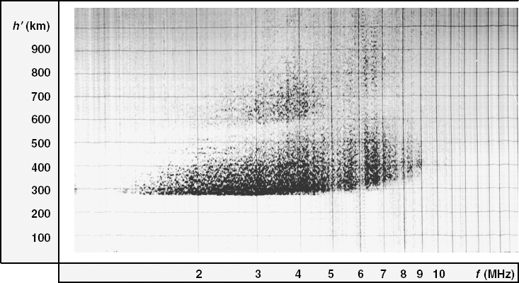
FIGURE 11.10 Ionogram for Huancayo at nighttime, with equatorial “spread-F”. (Courtesy of the National Geophysical Data Center, provided by Mr. Ray Conkright.)

Ionospheric sounding is a valuable research tool for probing the ionosphere. Many ionospheric sounding data are accessible through the Internet [3]. However, the main motivation for introducing ionograms here is to explain the puzzling peculiarities of ionospheric propagation, such as the skip and MUF phenomena. For this purpose, some additional theorems governing ionospheric propagation are needed. They are (1) the Secant law, (2) Breit and Tuve's theorem, and (3) one of Martyn's theorems, all to be considered next. It is important to note that they will be developed on the basis of plane stratification of the ionosphere, no Earth magnetic field effects, and lossless conditions. These are idealized assumptions that yield only an approximation of the actual situation, but a very useful one.

FIGURE 11.11 Ionogram for Huancayo at daytime, with “sporadic-E”. (Courtesy of the National Geophysical Data Center, provided by Mr. Ray Conkright.)

FIGURE 11.12 Ionogram for Churchill, Canada, at nighttime, with both sporadic-E and spread-F present. (Courtesy of the National Geophysical Data Center, provided by Mr. Ray Conkright.)

11.6 THE SECANT LAW

Consider two simultaneous propagation experiments, one oblique and the other vertical, with reflections occurring above the same point on the ground, as in Figure 11.13. The frequency of the oblique experiment f_ob is arbitrary. Let the height of highest penetration be h = h₁. Now let the frequency f_v of the vertical experiment be adjusted so that its height of penetration is also h₁ (this is a thought experiment, so let us not worry about how one would detect this condition). This frequency is called the equivalent vertical frequency. The Secant law states that the relationship between the oblique frequency and the equivalent vertical frequency is

FIGURE 11.13 Oblique and vertical waves.

Proof: For the oblique case, Snell's law gives

Neglecting loss and magnetic effects, and using (11.72) gives, in succession,

The vertical case is the limit of the oblique case as θ_I → 0, giving from equation (11.78)

so that f_N can be replaced with f_v to yield the Secant law, (11.74), which completes the proof.

Note that sec θ_I can also be defined from the geometry as

where D is the horizontal distance traversed by the curved oblique ray and h′ is a “virtual” reflection height defined by drawing a straight ray from the transmitter at angle θ_I up to the middle of the path. Later in the chapter, we will consider relationships between propagation along the straight ray/virtual reflection height path and along the curved ray path beyond the geometrical properties used here.

11.7 TRANSMISSION CURVES

Transmission curves are obtained from the Secant law and the geometry of a particular path. In what follows, a plane Earth geometry will be assumed for simplicity, although extension to the true spherical geometry is possible [1]. From the geometry and using the Secant law, it follows that

FIGURE 11.14 Transmission curves.

which can be solved for to yield

Transmission curves are plots created using equation (11.82). They show the virtual height h′ versus the equivalent vertical frequency f_v for a fixed value of distance D, and with the oblique frequency f_ob, that is, the candidate frequency to be used over this path, as a parameter. A typical plot is shown in Figure 11.14.

Transmission curves are useful because ionospheric propagation over path length D using frequency f_ob implies a reflection from the ionosphere at the virtual height h′ and equivalent vertical frequency f_v read from the transmission curve. This curve is determined entirely by the path geometry; still needed is information about the required state of the ionosphere to achieve propagation on this frequency for the specified path.

Note that the coordinates of transmission curves are vertical frequency and virtual height, just as they are for an ionogram. It would be tempting to superpose the transmission curves with an ionogram from the path midpoint. The frequencies of the ionogram can then be equated with the equivalent vertical frequencies of the oblique path. But such a superposition would be premature at this point. To be sure, the definition of equivalent vertical frequency guarantees that the true heights of reflection of the oblique and vertical waves are the same; however, it has not yet been shown that the virtual heights of the two are the same: we defined the virtual height using time delays on the vertical path, while the oblique virtual height has been defined using a straight ray geometry. In both ionograms and transmission curves, we have used the symbol h′ for virtual height, but until it is shown that these are indeed the same, this is merely sloppy notation!

FIGURE 11.15 Breit and Tuve's geometry.

11.8 BREIT AND TUVE'S THEOREM

The theorem of Breit and Tuve states that the time t required for a wave to travel over an actual ray path with maximum height h in the lossless, isotropic ionosphere is the same as the time t′ required for a ray, starting at the same incidence angle, to travel at the speed of light in vacuum over the corresponding virtual straight-line path with maximum height h′ at the center.⁴

Proof: From the geometry of Figure 11.15, the distance traversed by the virtual ray from the ground to height h′ is given by (D/2) csc θ_I. Since the virtual ray is assumed to travel at the speed of light in free space, the total travel time will be

For the actual ray, the element of time corresponding to the traversed distance ds is

By the use of (11.68), (11.69), and (11.63), this can be transformed to

and integration yields

where (11.83) has been used in the last step. This completes the proof of Breit and Tuve's theorem. We have found that the straight ray virtual path that was previously defined geometrically incurs the same time delay (assuming propagation in a vacuum) as the true curved ray path. The virtual path is therefore meaningful in a time delay sense. It still remains to determine relationships between the virtual reflection heights on the oblique paths and the equivalent frequency vertical path.

11.9 MARTYN'S THEOREM ON EQUIVALENT VIRTUAL HEIGHTS

Martyn's theorem on equivalent virtual heights states that, given an oblique transmission reflected from a lossless, isotropic ionosphere at some height h and the equivalent vertical transmission (i.e., at the equivalent vertical frequency and at the center of the path), the virtual reflection height of the oblique wave will be the same as the virtual reflection height of the equivalent vertical wave. This is equivalent to deriving a relationship between the time delays on the vertical and oblique true ray paths; the relationship obtained will enable the superposition of ionograms and transmission curves.

To prove the theorem, a preliminary lemma is required:

in a lossless, isotropic ionosphere.

Proof of Lemma: It follows from (11.72) that

Similarly, for the vertical wave the relation is

With the Secant law, f_v can be eliminated from (11.89) to give

which can be solved for

By substituting this into (11.88), using Snell's law (11.63) and some algebra, (11.87) is obtained.

Proof of Theorem: Let t_ob be the time required for the oblique wave to complete the travel from A to C in Figure 11.16 and let t_v be the time for the equivalent wave to travel up to the same true reflection point and back down. Then t_ob is given by

FIGURE 11.16 Martyn's theorem.

By the lemma, this becomes

The integrand in the last integral is just the differential of time, and the integral therefore gives t_v/2, yielding

By the theorem of Breit and Tuve, t_ob can be replaced with , the time taken by the virtual wave to travel the route ABC. Moreover, since the virtual ray is assumed to travel at velocity c, the quantity (ct_ob/2) is the distance AB. Therefore, the left-hand side of (11.94) becomes

and the result

follows, showing that the virtual height for an oblique propagation geometry is the same as that for the equivalent vertical frequency. Finally, here is the justification for superposing the ionogram and transmission curves!

11.10 MUF, “SKIP” DISTANCE, AND IONOSPHERIC SIGNAL DISPERSION

Figure 11.17 is an ionogram, neglecting magnetic field effects, superimposed on a set of transmission curves. The transmission curves specify the horizontal propagation distance and, via the Secant law, the physics of refraction. They contain no information about the particular ionospheric conditions. The ionogram, on the other hand, furnishes precisely that information. Together, that is, by the points they have in common, they determine the possibility of transmitting signals over the distance D at frequency f_ob.

FIGURE 11.17 Superposition of transmission curves and ionogram.

At frequencies f_ob above about 13 MHz, there are no points in common to the ionogram and transmission curves. Thus, if a frequency above 13 MHz is chosen as the operating frequency for these conditions, no signal will be received at distance D. No reception over this distance would be possible until the frequency is lowered to about 13 MHz. This frequency is called the basic maximum usable frequency (BMUF) for these ionospheric conditions and this propagation distance.

Referring again to Figure 11.17, at an operating frequency f_ob of 12 MHz, two propagation paths are possible, as shown by the intersections a and b. The ray corresponding to point b reaches a much higher virtual (and also actual) height than the one corresponding to a; it is called the high-angle or Pedersen ray. At 10 MHz, propagation is possible via a low-angle ray reflected from the F₁ region (intersection point c), a Pedersen F₁- region ray (intersection point d), and an F₂- region ray (intersection point e). However, the F₁ region reflections are unlikely to allow much energy to penetrate to the F₂ region, and the F₂ ray is therefore not likely to be effective; the F₂ region is said to be “screened” by the F₁ region for these conditions. At 6 MHz in Figure 11.17, E region transmission is possible, the F₁ layer is screened by the E layer, and transmission by F₂ reflection is impossible. Each ionospheric region and both the o- and x-waves (if magnetic effects are important) have their own maximum usable frequency. From Figure 11.17, the maximum usable frequency for F₁ transmission would be around 11 MHz. The notation F1(D)MUF is sometimes used to refer to these values, where D is the distance in kilometers. The BMUF is the highest of all these maximum usable frequencies.

In addition to the BMUF, it is a common practice to define the operational MUF (or simply MUF) as the highest frequency for which operation would be possible between two locations under a specific set of radio link conditions such as antenna gains, transmit power, required signal-to-noise ratio, and so on. The relative difference between the BMUF and the operational MUF is typically about 10–35%.

Because attenuation due to absorption decreases with frequency (as will be discussed later), it is tempting to operate just below the MUF. However, ionospheric conditions and hence the MUF depend on the season, hour of the day, geographical location, and sunspot activity. As a result, for propagation prediction purposes, the predicted MUF is taken as the monthly median of the observed MUF (also called the maximum observed frequency or MOF), that is, the highest frequency for which a skywave mode is available on 50% of the days in a month. This is equivalent to saying that, on any given day, communications may succeed at the predicted MUF only half of the time. To increase the probability of success, a suggested best operating frequency is chosen below the MUF. This latter frequency is known by various names such as frequency of optimum transmission (FOT), optimum working frequency (OWF), or optimum transmission frequency (OTF). For E and F₁ links, the FOT is taken as 95% of the MUF, while for F₂ links it is determined from a table in ITU-R Recommendation P.1239-1 [18]. Note that, while likely to be near optimum in a statistical sense, there is no guarantee that the FOT will be optimal, or even satisfactory, at a particular time.

An illustration of ray path changes, for a fixed distance, as frequency is varied is shown in Figure 11.18 for a simplified two-region ionosphere. At the highest frequency, f_a, the electron density in both layers is insufficient to cause the real part of the refractive index to vanish. Frequency f_a is above the critical frequencies of both layers, and the ray is not “reflected” and penetrates into space, with some refraction by both layers. As the operating frequency is lowered, the MUF of the top layer is reached, and below this value ray paths are shown for the o- and x-waves as sketched for frequency f_b. When the frequency is lowered below the MUF of the bottom layer, the ray paths are as shown for frequency f_d, and the upper layer is screened by the lower.

FIGURE 11.18 Ray paths for fixed distance D and varying frequency.

FIGURE 11.19 Ray paths for various distances at fixed frequency. (Adapted from Figure 4.6 of Davies, K., Ionospheric Radio Propagation, National Bureau of Standards Monograph 80, 1965.)

In Figure 11.18, the frequency was varied and paths for a specific distance D were considered. Actual antennas at MF and HF usually radiate over a wide range of vertical angles. Consider now the ray paths at a fixed frequency as a function of incidence angle on the ionosphere as in Figure 11.19. Assuming the operating frequency is greater than the critical frequency of the layer, a steeply incident ray (small incidence angle) will pass through the layer with little deviation, as shown by path 6. An increase in the incidence angle increases the deviation as shown by path 5a. A further increase in the incidence angle causes the ray to return at long distances as a high-angle ray, as in path 5. Such long distances can also be reached by a low-angle ray, path 1. Note that at large distances the high-angle ray path is very high and the low-angle path is very low. As the incidence angle is increased for the high-angle ray (path 4) or decreased for the low-angle ray (path 2), both rays return at increasingly shorter distances. Finally, there exists an incidence angle at which the high-angle and low-angle rays coalesce (path 3). This condition corresponds to point f in Figure 11.17.

This description of Figure 11.19 has used up all the incidence angles without any ray returning at a shorter distance than that of path 3. The transmission cannot be received at shorter distances! This minimum distance is called the “skip distance” for the particular frequency and ionospheric conditions. Points within that distance are said to be within the “skip zone”. From point f in Figure 11.17, it can be inferred that the frequency for which Figure 11.19 is drawn is the MUF for the skip distance. For points within the skip zone, the operating frequency is above the MUF, and communication can only be effected by lowering the operating frequency sufficiently. For a given oblique frequency, it is possible to predict the skip distance directly by overlaying the ionogram with transmission curves computed as D is varied for the specified f_ob. For this purpose, it is convenient to create transmission curves for a fixed oblique frequency with the path distance D as a parameter.

The high dispersion of ionospheric transmission, as evidenced by the strange and variable tone quality of analog voice transmissions, for example, can now also be explained. In general, there are four possible ionospheric ray paths from a transmitter to a receiver: high- and low-angle ordinary rays and high- and low-angle extraordinary rays. Wavelengths are on the order of tens of meters, while distances are hundreds or thousands of kilometers, that is, typically many thousand wavelengths. Therefore, it takes only a small change in the difference of refractive indices to greatly change the relative phases at the receiving site. At some sideband frequencies, the rays will add constructively, at others destructively, and this pattern changes as the ionosphere changes. Thus, wideband signals are distorted: the link is highly dispersive.

11.11 EARTH CURVATURE EFFECTS AND RAY-TRACING TECHNIQUES

The preceding discussion made three assumptions that served well to simplify the analysis and that work well in many (but not all) cases. First, we have often assumed that the ionosphere was lossless (Z = 0) and isotropic (i.e., Earth magnetic field effects were neglected). The results we have obtained remain approximately applicable in most cases even in the presence of these effects and require correction primarily for attenuation effects (as discussed later in the chapter) and to recognize the presence of the o- and x-waves.

Second was the assumption of a flat Earth. A misleading conclusion from this assumption is that paths are always available even for very large propagation distances. This is not true in reality because, for very large incidence angles θ_I, the Earth's curvature significantly changes the incidence angle at the ionosphere from that of a flat Earth. Typically, distances no larger than about 4000 km can be covered in “one-hop” ionospheric links, assuming ionospheric reflection at a height of about 400 km. For larger distances, multihop ionospheric propagation can be exploited; such links include several successive reflections at ionospheric layers and the Earth's surface along the path from the transmitter to the receiver [1,4].

The final assumption was that the ionosphere was horizontally uniform and a simple ray-tracing approach—as expressed by the theorems seen in this chapter—was applicable. More generally, there are situations where significant horizontal gradients may develop along the ionospheric propagation path. This is especially true, for example, during day/night transition times and away from mid-latitudes. In this case, more sophisticated ionospheric ray-tracing techniques can be employed [1,5,6].⁵ Ray-tracing techniques can be classified into analytical or numerical, depending whether the ray path integration is done numerically or analytically. Numerical ray tracing is in general more accurate but demands more computational resources than analytical ray tracing. A drawback for ray-tracing techniques is that they require very accurate ionospheric electron density models, beyond what is usually available in practice. Analytical ray-tracing techniques are still prevalently used in prediction tools for ionospheric propagation, as discussed in the next section.

11.12 IONOSPHERIC PROPAGATION PREDICTION TOOLS

As we have seen above, the behavior of a particular ionospheric link depends not only on the geographical locations of transmitter and receiver, but also on seasonal and diurnal variations and solar activity. Because of such spatial and temporal variability, it is difficult to apply the theory developed in this chapter for propagation prediction purposes without knowledge of the ionospheric conditions affecting the particular ionospheric link under consideration, at least in a statistical sense. As a result, various computer models for propagation prediction have been developed over the years based on detailed ionospheric description models [7, 8]. Perhaps the most widely used tools are those from the “IONCAP family,” that is, those derived from the Ionospheric Communications Analysis and Prediction Program (IONCAP) [9] developed by the Institute of Telecommunication Sciences of the National Telecommunications and Information Administration (NTIA) and its predecessors. This program also serves as the basis of ITU-R Recommendation P.533 for predicting the expected performance of HF skywave propagation systems [10]. A program, REC533, implementing this prediction model is available from the ITU-R, and ITU-R Recommendation P.533 gives a detailed account of the algorithms on which the program is based. Other members of the “IONCAP family” include the Voice of America Coverage Analysis Program (VOACAP)—an improved version of IONCAP first developed for the use by “Voice of America” radio broadcast stations—and the Ionospheric Communications Enhanced Profile Analysis and Circuit Prediction Program (ICEPAC)—an updated version of IONCAP with a more accurate model for the electron density profile [11], especially at higher latitudes, that includes geomagnetic effects such as those associated with aurora. VOACAP and ICEPAC are available from the U.S. Department of Commerce and provide detailed point-to-point graphs and area coverage maps for many parameters related to ionospheric propagation quality such as signal-to-noise ratio (SNR), signal power, and MUF. All the output parameters are based on monthly medians for given location(s), time of day, and solar activity (input parameters). Since they are all based on approximate models, these programs do not necessarily produce the same results. VOACAP and ICEPAC are similar for low latitudes, but differ at high latitudes. In the latter case, ICEPAC results are expected to be more accurate, and hence are recommended.

Figure 11.20 shows typical output data from VOACAP for illustrative purposes. REC533 and ICEPAC provide outputs in an identical format. Figure 11.20 displays geographical distributions of the MUF for a transmitter located in Columbus ,OH, at 1:00 PM (18:00 UT) for the month of June, assuming two levels of solar activities with annual sunspot numbers of 10 (low solar activity) and 100 (high solar activity), respectively. The scenario with a higher number of sunspots allows a larger MUF to be used because higher solar activity implies larger ion production—in other words, a more refractive ionosphere—as seen in Chapter 10.

11.13 IONOSPHERIC ABSORPTION

Ionospheric rays are attenuated by spreading as they propagate and may also be attenuated by absorption due to collisions. In terms of the refractive index, the specific attenuation α, in nepers per unit length, is given by

In the general case, n_I must be found from the Appleton–Hartree formula. Things become much simpler when the magnetic field is neglected, so that

which can be separated into real and imaginary parts as

Noting that

we can equate the imaginary parts of (11.99) and (11.100) to find

When this is used in (11.97) and X and Z are replaced with their definitions in (11.13) and (11.14), the result is

with N in electrons per cubic meter and ν and ω in rad/s.

No such simple formula can be given for the general case when the magnetic field is considered. However, for the Q_L case, it is found that a better approximation results if ω in (11.102) is replaced with ω ± ω_L, where the + sign refers to the ordinary ray.

Note that the specific attenuation decreases with frequency, so that operating at as high a frequency as is practically possible is desirable as discussed previously. From (11.102) it can be seen that there are two conditions for which attenuation will be relatively high. The first occurs when n_R is small. From Snell's law and the conditions for reflection, (11.63)–(11.65), it can be shown that this occurs near the point of reflection for near-vertical paths. This can be observed in the ionograms. Near the critical frequencies (cusps in the ionograms and reflection locations where N versus height is slowly varying), the wave traverses a longer effective distance for which n_R 0, resulting in high absorption. This is evidenced by the traces becoming faint near the cusps. Since the wave is “turning around” in this region, and hence deviating from a free-space path, this kind of absorption is called deviative absorption. The other condition for high absorption corresponds to large values of the product νN in (11.102). This product is largest in the upper D and lower E regions between 80 and 100 km because at lower altitudes there is not enough ionization and at higher altitudes the reduced density does not allow many collisions. It tends to be maximized at local noon because E region ionization correlates well with the solar zenith angle. This kind of absorption is called nondeviative. The reader may have noticed that transmissions in the 535–1606 kHz U.S. AM radio broadcast band can often be received at extremely large distances at night, but not so during daytime. The reason is that absorption prevents such reception in the daytime, but at night E region ionization disappears (N 0 in (11.102)), and the signal can then be received. Finally, it should be pointed out that ionospheric absorption can also increase sporadically, for example, due to increased electron densities in the D layer caused by solar flare events.

FIGURE 11.20 VOACAP prediction of the MUF in the month of June for transmissions from Columbus, OH, as a function of receiver location. The top and bottom plots use sunspot numbers of 100 and 10, respectively.

11.14 IONOSPHERIC EFFECTS ON EARTH–SPACE LINKS

Signals at VHF and above penetrate fully through the ionosphere, and a skywave mode of communication cannot be established. In this case, a “repeater station” (i.e., a satellite) can be employed for long-distance communication links, and the ionosphere acts primarily as a source of undesired perturbations on the Earth–Space signal. These perturbations are significant for frequencies up to 12 GHz and are particularly important for satellite links operating below 3 GHz.

The following types of perturbations may occur on Earth–Space propagation links crossing the ionosphere:

(a) Attenuation due to absorption.

(b) Faraday rotation, that is, the fact that a linearly polarized wave undergoes a rotation of the direction of polarization caused by the different phase velocities of right- and left-hand polarized waves in the ionosphere, as explained in Section 11.3.4. This is influenced by the total electron content (TEC) along the propagation path, as defined below.

(c) Group delay, also influenced by the TEC along the propagation path.

(d) Scintillations, that is, variations of the signal amplitude and phase due to small-scale ionospheric irregularities.

(e) Refraction, which causes a change in the apparent angle of signal arrival.

All of these effects except (b) are also present in the troposphere, but to a different degree and with a different dependence on frequency. In the following, we will discuss these five ionospheric perturbation mechanisms individually, focusing on their impact on trans-ionospheric propagation in the UHF and SHF bands.

Other ionospheric effects such as RF carrier advance, Doppler shift, and phase dispersion can also occur, but typically they are of a lesser importance and will not be considered here.

11.14.1 Faraday Rotation

The physical mechanism behind Faraday rotation was introduced in Section 11.3.4. Ignoring refraction and for frequencies where the lossless Q_L approximation holds, the differential phase difference due to the different phase velocities of the ordinary and extraordinary waves that is established along an infinitesimal path ds produces an infinitesimal rotation of the polarization angle.

Consider an polarized wave of unit amplitude propagating in the z direction as it enters the ionosphere:

Under the Q_L approximation, the characteristic polarizations are right- and left-hand circular; resolving this field into the characteristic polarizations yields

before entering the ionosphere. Each of the characteristic waves propagates at its own velocity in the ionosphere:

After propagating a small distance dz in the ionosphere (and defining z = 0 as the entry point), the field is

Now defining

we have

so that dΩ turns out to be, indeed, the incremental rotation angle. Using the Q_L approximation for n₊ and n₋ yields

Assuming frequencies sufficiently high so that the conditions Y_L 1 and X 1 hold, and using (1 + x)ⁿ 1 + nx for x 1, the above can be approximated as

and upon using (11.42), (11.43), (11.46), and (11.47), dΩ can be expressed as

where N(z) is the electron density per unit volume. Finally, integrating the above along the propagation path, we obtain the following expression for the Faraday rotation (radians)

where B_L = μ₀ H_L is the longitudinal component of the magnetic flux density, and T_ec is the TEC in the ionosphere along the propagation path defined by

The propagation path has been modified in the above to allow waves propagating in an arbitrary direction ds. Substituting the values of the physical constants in (11.112), we have

with Ω expressed in radians, f in hertz, B_L in tesla, and T_ec in electrons/m².

A plot of the Faraday rotation as a function of TEC and frequency is shown in Figure 11.21, assuming a high-latitude value of B_L = 54 μT. In the northern hemisphere, the Faraday rotation is counterclockwise as seen from an observer looking up. The average value of Ω has a cyclical (diurnal, seasonal, and solar cyclical) component that can be predicted and hence compensated by a proper adjustment of the relative tilt angle between the antennas. However, deviations from the average behavior occur as a result of geomagnetic storms that are difficult to predict. It should be noted that Faraday rotation occurs on the downlink as well as the uplink of an Earth–space system. To avoid Faraday rotation problems, circularly polarized antennas are often used since the characteristic polarizations undergo no changes during propagation and the characteristic polarizations are approximately circular when the Q_L approximation holds.

FIGURE 11.21 Faraday rotation as a function of frequency (in GHz) and TEC (in TEC units, where 1 TECU = 10¹⁶ electrons/m²) B_L = 54μT.

11.14.2 Group Delay and Dispersion

Due to the presence of charged particles, electromagnetic signals propagating through the ionosphere are slowed down compared to signals in a vacuum. The infinitesimal delay time dt experienced by a signal propagating along an infinitesimal path ds in the ionosphere is influenced by the local index of refraction and can be written as

where υ_g is the group velocity. In the VHF and SHF frequency bands, the quantities Y_L, Y_T, and Z are very small and can be neglected in the refractive index expression (11.61). X also is small, but neglecting it would remove the entire effect of the plasma and is therefore not permissible. As a result, the infinitesimal excess delay time with respect to vacuum, denoted as , becomes

where the fact that X is small has been used in expanding the square root by the binomial theorem. Substituting (11.42) and (11.46) in (11.116), we have

The total excess delay time is given by the integration of (11.117) along the propagation path, resulting with the use of (11.113) in

Substituting the values of the physical constants in (11.118), we have

with Δt^e expressed in seconds, f in hertz, and T_ec in electrons/m².

Figure 11.22 illustrates the percentage of yearly average daytime hours when Δt^e > 20 ns for a 1.6 GHz signal vertically incident on the ionosphere during a period of relatively high solar activity. The global distribution of Δt^e is influenced by the global T_ec distribution in the ionosphere. Since the excess delay time depends on frequency, different frequency components of a trans-ionospheric wideband signal will be subject to different delay times, resulting in dispersion. Figure 11.23 shows the difference in the time delay at the lower and upper frequencies of a pulse with temporal width τ centered at a specified frequency, for T_ec = 5 × 10¹⁷ electrons/m².

Group delays are a source of error in global navigation satellite systems such as the Global Positioning System (GPS) because they introduce an external bias source to the pseudorange, that is, the calculated “distance” between the GPS receiver and the GPS satellite. This distance is obtained from the satellite-to-receiver travel time: the range error Δρ is given by Δρ = c Δt^e.

FIGURE 11.22 Contours of the percentage of yearly daytime hours when Δt^e > 20 ns for a vertically incident 1.6 GHz signal, with sunspot number = 140. (Source: ITU-R Recommendation P.531-9 [12], used with permission.)

FIGURE 11.23 Difference in the one-way time delay between the lower and upper frequencies of the spectrum of a pulse of width τ transmitted through the ionosphere; pulse center frequency specified on vertical axis. (Source: ITU-R Recommendation P.531-9 [12], used with permission.)

11.14.3 Ionospheric Scintillations

Time-varying small-scale changes in the ionization density can cause fluctuations in the angle of arrival, amplitude, and phase of trans-ionospheric signals; these effects are called ionospheric scintillations and are analogous to similar effects in the troposphere discussed in Chapter 5. Here, we focus on the influence of ionospheric scintillations on signal amplitudes. Scintillation amplitudes greater than 15 dB are sometimes observed at 1 GHz. They decrease markedly at higher frequencies, and they vary greatly by geographical location. A detailed treatment is given in ITU-R Recommendation P.531-9 [12].

Statistics of the instantaneous variation of the signal intensity caused by ionospheric scintillations can be approximately described by a Nakagami-m probability density function [12], written as

where is the probability density function of the signal intensity (i.e., squared amplitude) ζ, Γ(m) is the gamma function, and the mean value of the intensity ζ is normalized to one, that is, . (The symbol indicates a mean value.) The m-coefficient of the Nakagami-m distribution is given by , where σ₄ is the “scintillation index” defined as

The scintillation index is related to the level of intensity fluctuations. As σ₄ approaches 1, the distribution of (11.121) approaches an exponential distribution for the intensity (corresponding to a Rayleigh distribution for the voltage magnitude, as seen in Chapter 8). Sometimes, σ₄ > 1 can occur due to wave focusing by the irregularities. For engineering purposes, a more descriptive parameter than the scintillation index is the fluctuation in the peak-to-peak signal intensity expressed in dB, denoted as I₄. The relationship between these two parameters can be approximated through . Table 11.1 compares a few values of σ₄ and I₄.

The fading rate of ionospheric scintillations tends to vary from about 0.01 Hz to about 1 Hz. A “power spectral density” plot decomposes signal fluctuations into component frequencies, so that the relative contributions of fluctuations on different timescales can be discerned. Figure 11.24 illustrates a typical power spectral density of the scintillation in a geostationary satellite link at 4 GHz; higher values of the power spectral density indicate that signal fluctuations at the associated frequencies are more predominant. The power spectral density of the scintillations in Figure 11.24 exhibits a large range of frequency dependencies, with the fluctuation strength decreasing rapidly as their frequencies become higher (timescales become shorter.) Observations with dependencies ranging from 1/f to 1/f⁶ have been reported. In the absence of direct measurement data, ITU-R Recommendation P.513-9 suggests using 1/f³ for system applications [12]. Strong scintillations usually do not occur continuously but in distinct scintillation events. Ionospheric scintillations are more pronounced around a 20°-wide latitude ring centered on the geomagnetic equator, where they tend to occur predominantly in the late evening and early morning, and in regions above latitude 55°, where there is no preferential time and the behavior is more irregular.

It should be pointed out that the combined presence of rain attenuation, studied in Chapter 5, and ionospheric scintillation can cause effects—particularly in equatorial regions where both are stronger—that neither alone can produce. For example, the combination can produce significant fluctuation in the cross-polarization signal, even though rain attenuation does not cause significant signal fluctuations and ionospheric scintillation does not cause significant depolarization.

TABLE 11.1 Conversion Table Between Some Values of the Scintillation Index σ₄ and the Intensity Fluctuation Expressed in dB

σ4	I4 (dB)
0.1	1.5
0.2	3.5
0.5	11
0.8	20
1.0	27.5

Source: ITU-R Recommendation P.531-9 [12].

FIGURE 11.24 Power spectral density of the ionospheric scintillation for a 4 GHz geostationary satellite link. Note the 1/f³ behavior visible in the 0.1–1 Hz frequency range. The six different curves labeled A–F refer to a sequence of measurements taken 30 min or 1 h apart. (Source: ITU-R Recommendation P.531-9 [12], used with permission.)

11.14.4 Attenuation

We have previously considered ionospheric absorption in Section 11.9 when we discussed the conditions for deviative and nondeviative absorption. For trans-ionospheric signals at VHF band and above—where ω is much greater than the collision frequency ν—the attenuation constant α in (11.102) can be approximated as

where n_r 1 (no refraction) was also used. Under these conditions, the total attenuation in dB for a one-way traverse of the ionosphere will be proportional to 1/f². For vertical links at 30 MHz, for example, the typical (mid-latitude) ionospheric one-way attenuation due to absorption is on the order of 0.2–0.5 dB. At 1 GHz and above, the absorption is below 0.01 dB and hence can be neglected.

11.14.5 Ionospheric Refraction

The skywave mode is a consequence of strong ionospheric refraction that bends upgoing rays at MF and HF back toward the Earth. At higher frequencies, refraction causes a change in the apparent angle of arrival ϕ_a from the satellite signal at the ground terminal, but the change is generally small compared to the beamwidth of the ground station antenna and therefore usually has little effect on system operation. The amount of ionospheric refraction depends on the electron density distribution along the ray path and, for identical propagation conditions, the error in the apparent angle of arrival decreases with the square of the frequency in the VHF to SHF bands, similar to the behavior of the Faraday rotation and the group delay.

At 1 GHz, the error in the angle of arrival of a signal with elevation angle of 30° is less than 0.06 mrad. Table 11.2 lists some approximate peak ionospheric perturbations for (one-way) trans-ionospheric links in a few selected frequencies in the UHF and SHF bands. An elevation angle of 30° is assumed.

11.14.6 Monitoring TEC Distribution

We have seen that the TEC is a very important parameter in determining the effect of ionospheric perturbations on trans-ionospheric links. The TEC in (11.113) refers to total electron content integrated along the ray path from the satellite to the ground terminal. This is also referred to as the “slant TEC”, as opposed to the “vertical TEC”, which is integrated along a zenith path. The vertical TEC typically varies between 10¹⁶ and 200 × 10¹⁶ electrons/m² and is often expressed in TEC units (TECU), where 1 TECU = 10¹⁶ electrons/m², as in Figure 11.21. For prediction purposes, estimates for the vertical TEC can be obtained from computer models, such as the International Reference Ionosphere (IRI) model or the NeQuick ionospheric model mentioned in Chapter 10.

TABLE 11.2 Approximate Peak Ionospheric Perturbation Effects

FIGURE 11.25 Map of the distribution of the vertical TEC over North America, under quiet (top) and stormy (bottom) ionospheric conditions. (Source: Ref. [17].)

Neglecting refraction effects and for a sufficiently small off-zenith satellite look angle γ (so that the Earth curvature can be neglected and the ionosphere can be assumed horizontally stratified) the vertical TEC, , can be related to the slant TEC, T_ec, via

One possible technique for monitoring the temporal (due to diurnal, seasonal, and solar cycle effects) and spatial (geographic) variability of the vertical TEC is by relying on a network of dual-frequency ground receivers of global navigation satellite systems such as GPS [14]. The dispersive nature of the ionosphere allows TEC estimation by GPS observations at two frequencies in the same location through equation (11.119)—here using the GPS error due to the ionosphere as a source of TEC information! Another possible technique for TEC monitoring is through the use of low-Earth orbit satellites that exploit radio occultation techniques relying on radio signals from GPS transmitters [15]. Finally, ground-based ionosonde data can also be used to estimate vertical TEC by carefully extrapolating the measured vertical electron density profile beyond the inflection point [16].

Figure 11.25 plots the vertical TEC (measured in TECU) over North America on 2 days: 10/28/2003 at 21:15UT (top) and 10/29/2003 at 21:00UT (bottom) from data obtained through a network of GPS stations operated by the U.S. National Geodetic Survey, NOAA[17]. The observed TEC values from the top map (in the range of about 50 TECU) are fairly typical in the late afternoon. In contrast, the bottom map shows the ionosphere about 24 h later, in the middle of an extremely strong ionospheric storm, with TEC values above 200 TECU in parts of central Mexico.

REFERENCES

 1. Davies, K., Ionospheric Radio, IEE Electromagnetic Wave Series 31, Peter Peregrinus Ltd., London, 1989.

 2. Milsom, J., “Surface waves, and sky waves below 2 MHz,” in Propagation of Radiowaves, second edition (L. Barclay, ed.), pp. 357–383, The Institution of Electrical Engineers, London, 2003.

 3. Reinisch, B. W., I. A. Galkin, G. Khmyrov, A. Kozlov, and D. F. Kitrosser, “Automated collection and dissemination of ionospheric data from the digisonde network,” Adv. Radio Sci., vol. 2, pp. 241–247, 2004.

 4. Boithias, L., Radiowave Propagation, McGraw-Hill, New York, 1987.

 5. Bennet, J. A., “Some reflections on the ray tracing of radio rays in the ionosphere,” Radio Sci. Bull., no. 327, pp. 10–12, 2008.

 6. Cannon, P. S., and P. A. Bradley, “Ionospheric propagation,” in Propagation of Radiowaves, second edition (L. Barclay, ed.), pp. 313–334, The Institution of Electrical Engineers, London, 2003.

 7. Rush, C. M., “Ionospheric radio propagation models and predictions–a mini-review,” IEEE Trans. Antennas Propagat., vol. 34, no. 9, pp. 1163–1170, 1986.

 8. Cannon, P. S., “Ionospheric prediction methods and models,” in Propagation of Radiowaves, second edition (L. Barclay, ed.), pp. 335–355, The Institution of Electrical Engineers, London, 2003.

 9. Teters, L. R., J. L. Lloyd, G. W. Haydon, and D. L. Lucas, “Estimating the Performance of Telecommunication Systems Using the Ionospheric Transmission Channel—Ionospheric Communications Analysis and Prediction Program User's Manual,” National Telecommunication and Information Administration, Report NTIA 83–127, Boulder, CO, 1983.

10. ITU-R Recommendation P.533-9, “Method for the prediction of the performance of HF circuits,” International Telecommunication Union, 2007.

11. Tascione, T. F., K. W. Kroehl, and B. A. Hausman, “A technical description of the ionospheric conductivity and electron density profile model (ICED version 196-II),” Syst. Doc vol. 7, Air Force Weather Agency, Scott Air Force Base, Illinois, 1987.

12. ITU-R Recommendation P.531-9, “Ionospheric propagation data and prediction methods required for the design of satellite services and systems,” International Telecommunication Union, 2007.

13. ITU-R Recommendation P.618-9, “Propagation data and prediction methods required for the design of Earth–Space telecommunication systems,” International Telecommunication Union, 2007.

14. Liu, Z., S. Skone, Y. Gao, and A. Komjathy, “Ionospheric modeling using GPS data,” GPS Solutions, vol. 9, no. 1, pp. 63–66, 2005.

15. Angling, M. J., and P. S. Cannon, “Assimilation of radio occultation measurements into background ionospheric models,” Radio Sci., vol. 39, no. 1, RS1S08, 2004.

16. Reinisch, B. W., X. Huang, A. Belehaki, and R. Ilma, “Using scale heights derived from bottomside ionograms for modelling the IRI topside profile,” Adv. Radio Sci., vol. 2, pp. 293–297, 2004.

17. Spencer P. S. J., D. S. Robertson, and G. L. Mader, “Ionospheric data assimilation methods for geodetic applications,” Position, Location, and Navigation Symposium 2004, Proceedings, pp. 510–517, Monterey, CA, April 26–29, 2004.

18. ITU-R Recommendation P.1239-1, “Reference ionospheric characteristics,” International Telecommunication Union, 2007.