
5
DIRECT TRANSMISSION
5.1 INTRODUCTION
In general, the propagation of a transmitted signal may be affected by interactions with the environment in which the signal propagates (such as reflection and refraction as will be discussed in Chapter 6). In many systems of practical importance, interactions with the environment do not cause significant changes in the signal propagation. The term “direct transmission” is meant to designate such situations; this propagation mechanism is dominant for many satellite communication and radar systems.
In this chapter, the Friis transmission formula for prediction of signal strength under ideal direct transmission conditions is derived. Calculation of attenuation due to atmospheric gases is then discussed, on both vertical and slant paths. A model for predicting rain attenuation and the expected system outage time for a given “rain margin” follows. Methods of improving system performance through diversity and the scintillation phenomena that occur on paths through the atmosphere are then discussed. Finally, a derivation of the look angle from a specified point on the Earth's surface to a geostationary satellite is given in the appendix of this chapter because of the importance of the direct transmission mechanism in satellite communications applications.
5.2 FRIIS TRANSMISSION FORMULA
Consider an isotropic radiator, which is a conceptual antenna that radiates energy equally in all directions. Such antennas do not exist in practice; nevertheless, the concept is useful. Note that an omnidirectional antenna is one that radiates nearly equally well in all the directions of one plane, for example, in azimuth, but that has a directional, though generally broad, radiation pattern in the orthogonal plane. Omnidirectional antennas are used in practice. It is important not to confuse “isotropic” and “omnidirectional.”
Consider an isotropic radiator in an ideally simple medium. Since neither the antenna nor the medium imparts any directionality to the radiated power, the radiated power flux density will be a function only of the distance R and, by power conservation, is given by
where PT is the power input to the transmitting antenna and υT is its radiation efficiency. The subscript T is used above because both a transmitting and a receiving antenna will be needed in an application.
The directional gain D(θ, ϕ) of an antenna is defined as the ratio of the power flux density radiated in the direction (θ, ϕ) to that which would be radiated by an isotropic radiator. Thus, the power density radiated by a directive antenna is obtained from equation (5.1) as
where the last step follows from the relation between gain G and directional gain D.
For transmitting and receiving antennas separated sufficiently so that far-field conditions (4.1) are satisfied, according to equation (4.31) the power delivered to the terminals of the receiving antennas will be
where AR is the receiving aperture (or receiving area) of the receiving antenna. Note that the coordinates (θT, ϕT) are those at which the receiving antenna appears when viewed in the coordinate system of the transmitting antenna, while (θR, ϕR) are those of the transmitting antenna in the coordinate system of the receiving antenna.
In microwave systems, it is customary to match the receiving antenna to its receiver and also to match the receiving antenna polarization to the received field (the polarizations may be mismatched in interference calculations.) If both the impedance and the polarization are matched, the receiving aperture AR becomes equal to the effective area Ae of the receiving antenna,

where equation (4.35) has been used for the second equality. Equation (5.3) now becomes

where the wavelength λ and the distance R must be in the same units. This equation is known as the Friis transmission equation. It is the basis for many system calculations. Note that the arguments (θ, ϕ) of GT and GR are often omitted.
Since the ratio of PT to PR is generally large, decibel notation is often used for system calculations. In decibel notation, with the use of
the result is
In this expression, the notation PT,dbW, PR,dbW indicates that both the transmitted and received powers are specified in decibels relative to 1 W. Often decibels relative to 1 mWare used instead; in this case, the notation PT,dbm, PR,dbm is used. Note that the units for distance and frequency are km and MHz, respectively.
5.2.1 Including Losses in the Friis Formula
The Friis transmission equation takes no account of any losses in the transmission medium that may attenuate the signal. In the atmosphere, loss can generally be neglected in the frequency range from 100 MHz to 5GHz and, except for heavy rain, even up to 10 GHz. In the frequency range above 10 GHz, two loss effects become important. The first is due to gases, specifically water vapor and oxygen, whose molecules exhibit resonances at these frequencies and can therefore convert energy from the transmitted wave into heat, thus causing the wave to be attenuated. The second is due to hydrometeors, that is, liquid or solid water, such as rain, snow, and fog, with rain generally the most important because liquid water absorbs more strongly than ice in the microwave frequency range. Finally, the Friis transmission equation has neglected impedance and polarization mismatches. Taking all these considerations into account transforms equation (5.5) into

The Timp and Tpol factors represent impedance and polarization mismatches, as in equation (4.30). The transmission factor due to gases Tgas can be calculated from a “specific extinction coefficient” for gas absorption αgas as

where αgas is measured in nepers per unit length and Tgas is the fractional transmission (e.g., 0.5 for 50% transmission).
Similarly the rain transmission factor Train can be obtained from a specific extinction coefficient due to rain as

It is easy to see that transmission factors are multiplied to obtain the total transmission of several layers. If the first layer transmits 90% of the power and the second layer transmits 80% of what it receives, then the total transmission is 0.9 × 0.8 = 0.72, or 72%. The logarithmic nature of αgas converts the multiplication to addition, and the integral represents the addition of infinitely thin layers. From (5.9) it is seen that power density decreases exponentially in a homogeneous medium.
The antenna-to-medium coupling factor Tcoup comes into play when the transmission medium modifies the usual antenna pattern, for example, when GT(θT, ϕT) represents a free-space antenna pattern, but the antenna is used for ionospheric transmission. For direct transmission Tcoup = 1.
It is more common to express the relations of equation (5.8) in decibel notation, similar to equation (5.7),
where the system loss Lsys,db is given by

The losses in equation (5.12) can be obtained from the corresponding transmission factors in equation (5.8) by
The attenuation due to gases in decibels (defined to be a positive number if loss occurs) can also be found from a specific attenuation in dB as

and that for rain from

It is easy to show that the relationship between the specific extinction coefficient, α, usually measured in nepers/km, and the specific attenuation, αdb, usually measured in dB/km, is

Because of the simpler form of equations (5.14)–(5.15) compared to equations (5.9)–(5.10), it is generally preferred to use the specific attenuations αgas,db and αrain,db, defined as the attenuation in decibels per unit distance, usually specified in dB/km. These quantities are discussed in more detail in the following sections. Polarization and impedance mismatch losses are obtained from Chapter 4 as

In using the logarithmic form, it is useful to have a feel for the range of values to be expected. When a calculation falls out of the expected range, one should suspect an error in the calculation! A brief example will demonstrate practical system loss limits. A large transmitter might transmit a megawatt. A sensitive receiver with 100Ω input impedance might detect 1 μV (rms). For these values, a system loss of up to 10 log10 106/ ((10−6)2/100) = 200 dB would be tolerable. Thus, the practicality of PT/PR ratios much greater than 200 dB should be questioned.
In this section, the distinction between natural and decibel quantities has been denoted carefully by subscripts, for example, Tgas and Lgas,db, for describing the attenuation due to atmospheric gases. Such a convention will also be followed in the rest of this chapter. In the literature, such a careful distinction is seldom found; the reader is expected to understand which is meant from the units or the context.
5.3 ATMOSPHERIC GAS ATTENUATION EFFECTS
The specific attenuation αgas,db in dB/km for a standard atmosphere at sea level (surface water vapor content of 7.5 g/m3 and surface temperature 20° C) is plotted in Figure 5.1, using the methods described in ITU-R Recommendation P.676-7 [1]. The multiple curves in the plot describe the contributions of atmospheric water vapor and oxygen separately, as well as the combined attenuation of these two effects. Note that water vapor dominates at and near sea level for frequencies greater than 100 GHz, so that the “both” and “water vapor” curves coincide. The peaks at 22.2, 183.3, 325.4 GHz, and higher frequencies are due to water vapor and would be greatly reduced for a very dry climate; those at 60 and 118.7 GHz are due to oxygen. The attenuation near the peaks can be so high as to make the atmosphere virtually opaque; the frequency regions where the attenuation is not excessive are often referred to as “windows” in the atmosphere, for example, the windows near 40 and 90 GHz. Attenuation due to water vapor shows an increasing trend with frequency, so the impact of water vapor (when present) is significant at all frequencies greater than 100 GHz.

FIGURE 5.1 Atmospheric specific attenuation versus frequency, at or near sea level.
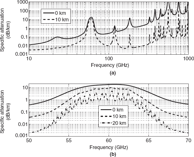
FIGURE 5.2 (a) Specific attenuation at varying altitudes. (b) Specific attenuation by atmospheric oxygen at varying altitudes.
Figure 5.2a compares the total atmospheric specific attenuation at sea level with that at altitude 10 km. Two features are important to observe here: first, the decreased attenuation observed in the 10 km case is largely due to the decreased concentration of water vapor at higher altitudes. Second, the absorption peaks (or “resonances”), for example, near 118.7 or 183.3 GHz, are sharper at 10 km than at sea level due to a mechanism called “pressure broadening.” Collisions with other atmospheric molecules can broaden the resonant behavior of atmospheric gas absorption; these effects are more significant at lower than higher altitudes due to the increased atmospheric pressure at lower altitudes. Both these effects make clear that it is important to take the altitude dependence into account (as described in ITU-R P.676-7) when computing the specific attenuation due to atmospheric gases.
A more vivid example of pressure broadening effects is provided in Figure 5.2b, which illustrates the specific attenuation due to atmospheric oxygen near the 60 GHz resonance. The curves illustrated for multiple altitudes show that the broad peak at sea level actually is due to many fine lines that merge due to pressure broadening at the lower altitudes.
5.3.1 Total Attenuation on Horizontal or Vertical Atmospheric Paths
When a long vertical or slant path through the atmosphere is under consideration (for example, to a satellite), the total attenuation must be ascertained by integrating the specific attenuation over the path. The total attenuation due to atmospheric gases for horizontal paths is obtained by integrating the specific attenuation over the path
where L is the path length, and the last equality stems from the fact that the specific attenuation seldom varies greatly in the horizontal direction. Such a simple relationship for vertical or slant paths is not possible, however, due to atmospheric variations with altitude.
Precisely vertical paths are uncommon in practice, but they provide a useful starting point for considering the common case of slant paths through the atmosphere, for example, in satellite communications. Results of a calculation for a vertical path beginning at various altitudes are shown in Figure 5.3. An interesting feature of these curves is that the resonance absorption peaks narrow for increasing altitude due to the collision broadening mechanism discussed earlier.
To calculate the curves of Figure 5.3, distributions of oxygen and water vapor densities as a function of height must be known or assumed. One approximation is an exponential distribution; for example, for water vapor density the function
is often used, where ρ0 is the water vapor density at sea level, h is the altitude of interest, and hs,w is called the scale height for water vapor, with a typical value of approximately 2 km. Use of an exponential function of altitude for many atmospheric properties is justified by the “barometric law” discussed in Chapter 10. For water vapor, such approximations can be good in a statistical sense for altitudes up to about 8 km and can also usually be used on paths from a low altitude through the atmosphere because nearly all the attenuation occurs at low altitudes. On the other hand, use of equation (5.20) would certainly be a poor assumption for calculating the attenuation from a stratospheric balloon to a satellite! Another approach is the use of a “model atmosphere,” that is, an empirical model of atmospheric properties versus altitude based on theory and measurements.

FIGURE 5.3 Total attenuation from specified height to top of atmosphere, ITU-R Standard Atmosphere (7.5 g/m3 water vapor concentration at sea level).
The actual calculation of the attenuation due to gases on a zenith path through the atmosphere can then be performed by integrating the specific attenuation for the specified atmospheric composition over height. Results are commonly presented as an equivalent height by which the specific attenuation due to the gas at the lowest altitude must be multiplied to yield the actual attenuation. More information on such calculations can be found in ITU-R Recommendation P.676-7 [1]. The complexity of such calculations is seldom required. Useful estimates of total attenuation on a vertical path through the atmosphere can be obtained from Figure 5.3.
5.3.2 Total Attenuation on Slant Atmospheric Paths
On slant paths with elevation angles greater than about 10° above the horizon, the curvature of the Earth may be neglected. In that case, the relationship between vertical and slant attenuation in dB can be derived readily from the geometry of Figure 5.4. For the vertical path, the attenuation is given by

in dB, while for the slant path, the corresponding expression is


FIGURE 5.4 Slant path geometry.
in dB. Since θ is a constant over the path, the cosecant may be taken outside the integral, and the result is
in dB. As a corollary, the attenuations for two different elevation angles θ1 and θ2 are related by

The cosecant law and its corollary are not valid for elevation angles less than about 10°. For lower elevations, Earth curvature must be taken into account, and so must refraction since a small angular deviation may cause a considerable change in the path length. Expressions for treating this case may be found in ITU-R Recommendation P.676-7 [1].
5.3.3 Attenuation at Higher Frequencies and Further Information Sources
The preceding discussion has been centered primarily on the microwave portion of the spectrum, where the atmosphere is largely transparent except for the oxygen and water vapor line frequencies. However, the molecular components of the atmosphere have a much larger number of resonances at frequencies greater than 300 GHz, and greater consideration must be given to atmospheric gas attenuation. Even Figure 5.3, which considers only oxygen and water vapor attenuation, shows that the low atmospheric attenuation obtained for frequencies below around 300 GHz (with the exception of the oxygen and water line frequencies) increases rapidly beyond this limit. Communication and radar systems intended to exploit these frequencies must therefore be designed to overcome substantial atmospheric attenuation.
Calculations based on the information given above yield only rough estimates of atmospheric attenuation. ITU-R P.676-7 gives detailed instructions for more precise calculations in the frequency range 1–1000 GHz, with a simplified procedure for 1–350 GHz. A computer program is also available from the ITU-R. Propagation at higher frequencies including the infrared, visible, and ultraviolet spectrum is beyond the scope of this book. Computer codes for these spectral regions include the FASCODE and MODTRAN programs for moderate resolution and the proprietary Hitran-PC code for high resolution, as is needed for laser applications. They are based on the HITRAN database for molecular resonance line parameters. Access to these codes has changed over the past few years; the reader is encouraged to use the Internet for more details, where references to other specialized codes in these spectral regions may also be found.
5.4 RAIN ATTENUATION
The water vapor discussed in the preceding section is water in its gaseous state. Water can also exist in its liquid or solid state in the atmosphere, in the form of rain, snow, fog, clouds, ice, and so on. “Hydrometeors” is the general term for nongaseous water in the atmosphere. Of these, rain is the most significant factor in propagation analyses for two reasons. The first is that liquid water absorbs more electromagnetic energy at microwave frequencies than ice or snow. The second is the fact that the sizes of liquid water particles for rain are much larger than those in clouds or fog (which usually have radii smaller than 100 μm), leading to increased attenuation effects. We therefore focus on rain attenuation in the following discussion. Information on attenuation by other hydrometeors is provided in ITU-R Recommendation P.840-3 [2], and would generally be of concern only when small attenuation values are of interest, and at frequencies greater than approximately 30 GHz.
Rain attenuation is highly variable in time, in its vertical and horizontal extent, and from location to location. Its impact can usually be neglected at frequencies below 5 GHz, but becomes increasingly important at higher frequencies. Because it remains impossible to predict the occurrence of rain with certainty, rain attenuation is usually described by statistical means: that is, the rain attenuation for a given location is modeled as a random variable. A more formal description of random variables and their properties is provided in Chapter 8. For the purposes of this chapter, it is sufficient to understand that our goal is to obtain an estimate of the number of hours per year (or equivalently the annual percentage of time) that a given amount of rain attenuation will be exceeded at a given location. Such information can be used in system design to plan for enough transmit power so that rain attenuation causes insufficient received power for only a very low percentage of the time. Calculations of this sort are known as “rain margin” or “system reliability” analyses.
Figure 5.5 provides an example of a rain attenuation distribution, in this case computed for an Earth–space path where the Earth station is at sea level and at latitude 40°, and for specified location rain statistics (discussed in what follows). The horizontal axis represents the number of hours per year (on average) that the rain attenuation indicated on the vertical axis is exceeded. For example, for path elevation angle θ of 20°, and at 14 GHz, we can see that a rain attenuation of 3 dB is expected to be exceeded around 10 h per year. Such information is very useful in assessing the impact of rain on system performance. It is not surprising that the curves in Figure 5.5 decrease from left to right, as higher rain attenuations (very heavy rain) are encountered less frequently than smaller rain attenuations (light rain). The dependencies on frequency and path elevation angle shown in Figure 5.5 will become clearer further on. The curves of Figure 5.5 are applicable for a specific location and must be recalculated for different locations of the Earth station to take into account local climate effects on rain properties.

FIGURE 5.5 Sample rain attenuation distributions for station latitude 40°, station height 0 km, and Rr,0.01 = 49 mm/h.
In order to reach the goal of producing rain attenuation distributions, we begin with a physical description of the rain itself, consider the mechanisms of rain specific attenuation, and present a simplified model for this quantity. We then consider the requirements for computing the total rain attenuation over a specified path, but again will find it necessary to resort to an empirical model for this process, due to the difficulty of obtaining the statistics of the physical processes involved. For example, it is difficult to measure raindrop shape and size distributions, and such measurements have been performed only at relatively few locations and over limited time spans. In contrast, measurement of the attenuation of a satellite signal is relatively simple and, within limits, the attenuation can also be inferred from radiometric measurements of the noise emitted from the rain. Thus, a relatively large database of rain attenuation statistics is available for fitting an empirical model. Methods for describing statistics of rain attenuation at a given location are also discussed.
5.4.1 Describing Rain
The simplest description of rain is an atmosphere that contains a given number of water particles, all of the same shape, size, and orientation, uniformly spread through a region of space. Unfortunately, this description is not sufficient for rain, as raindrops vary in all three of these properties, and variations in raindrop size, in particular, have an important impact on attenuation. Neglecting shape and orientation effects for the moment by modeling the raindrops as spherical, it is possible to describe rain in terms of a “drop size distribution”: n(r)dr is the number of raindrops contained in a unit volume of the atmosphere that are within an interval dr of the drop radius r. According to this definition, the total number of raindrops per unit volume is then

and n(r) is usually reported in units of “per cubic meter per millimeter” with r in millimeters, resulting in N being the number of drops per cubic meter. It is also possible to compute the fraction of the atmospheric volume that is occupied by liquid water as

where the factor of 1000 is included assuming the units of n(r) are per cubic meter per millimeter and r is in millimeters.
Numerous measurements of the drop size distribution have been performed. One model that is widely used (but not necessarily the ideal model in all situations) is that of Marshall and Palmer: [3, 4]
where N0 = 16000 and ![]() when n(r) has units of per cubic meter per millimeter and r is in millimeters.
when n(r) has units of per cubic meter per millimeter and r is in millimeters.
Here, Rr (the only parameter needed by this distribution to specify rain properties) is the “rain rate” measured in units of millimeters per hour. This quantity specifies the number of millimeters of rain that would be captured in an open, vertically oriented, container of uniform cross section over a period of 1 h. Rain rates of 5 mm/h or less represent a light rain, while rain rates up to 100 mm/h or more can occur for brief periods during strong thunderstorms.
One issue in using the Rr parameter involves the duration of the measurement. For example, it would be highly unlikely to observe an Rr of 100 mm/h or more if the rain measurement is performed over a duration of 1 h because such heavy rains occur only over shorter periods of time. Nevertheless, such short periods of time can be important in examining system reliability! For this reason, it is common in propagation analyses to use rain rates Rr in mm/h that represent measurements performed over a period of 1 min.
Figure 5.6 provides a plot of the Marshall–Palmer drop size distribution for two rain rates. Both curves show a decrease in the number of particles per unit volume for larger drop sizes, but the high rain rate case shows a shift toward larger drop sizes in general. Using the Marshall–Palmer distribution, we can find

FIGURE 5.6 Marshall–Palmer drop size distribution for two rain rates.
showing that, even at high rain rates, the fractional volume occupied by liquid water in the atmosphere is very small.
If the assumptions to this point are accepted, then the description of rain properties reduces to a description of the rain rate Rr as a function of both horizontal and vertical space. Rain rate at the Earth's surface is a commonly measured meteorological quantity, and extensive data sets are available for this parameter, for example, from the National Weather Service or the National Oceanographic and Atmospheric Administration (NOAA) in the United States. Such information can be used to represent rain rate at a given location as a random variable, and the property of most interest in propagation analysis is the percentage of time that a given rain rate is expected to be exceeded at a specific location. Rain rate analyses using globally compiled data sets have shown that rain statistics can often be adequately modeled as a combination of two processes: normal rain and thunderstorm rain, with the latter contributing mostly to the higher rain rates. Current models for rain attenuation effects usually consider only the rain rate that is exceeded 0.01% of the time (i.e., 52.6 min/year) at a given location, called Rr,0.01. ITU-R Recommendation P. 837-5 [5] provides a global database for estimating Rr,0.01; local measurements of such information are preferable if they are available. Figure 5.7 provides a contour map of Rr,0.01 for the continental United States.

FIGURE 5.7 Shaded contour plot of Rr,0.01 (mm/h) for the continental United States, using data from ITU-R P. 837-5.
5.4.2 Computing Rain Specific Attenuation
The extremely low fractional volume of raindrops in the atmosphere enables computation of rain specific attenuation using an “independent scatterer” assumption. This method assumes that the power lost by a radiowave propagating through rain is simply the sum of all the powers lost in the individual raindrops; that is, there is no shadowing of one raindrop by another or multiple scattering. Determining the power loss per unit volume then reduces to an integration of the power lost for each drop over the drop size distribution, since drops of different sizes absorb different amounts of power.
When a radiowave encounters a single raindrop, two effects cause loss of power. The first is absorption of power inside the raindrop. Since water is a lossy medium at microwave frequencies, this absorption is an important cause of attenuation in rain. The second effect is scattering of the radiowave by the raindrop that causes some of the radiowave energy to be redirected into propagation directions other than the original direction. The sum of these two effects is called the “extinction” caused by the raindrop.
Computing the scattering and absorption of incident radiowave power for a given scatterer is a classical electromagnetic problem. For scatterers that are very small compared to the wavelength of the radiowave, the Rayleigh approximation [6] shows that the extinction of a particle is proportional to its volume squared. Thus, larger radius raindrops are much more important than smaller drops in determining attenuation. The Rayleigh approximation can be used for rain at frequencies up to approximately 10 GHz.
At higher frequencies, other methods for predicting the extinction of a specified scatterer are required. The Mie theory [6] describes the extinction of a spherical scatterer of arbitrary size in terms of an infinite series summation. The Mie theory shows that the extinction eventually becomes a quadratic function of the scatterer radius as the particles become larger compared to the electromagnetic wavelength, so that larger raindrops, while still important, are less dominant than in the Rayleigh scattering case.
Using either the Rayleigh or the Mie theory as applicable to compute the extinction of a single raindrop, the average extinction for rain of a given rain rate can be computed by averaging these extinction values over the drop size distribution. Such approaches usually require a numerical integration to predict the specific attenuation as a function of the rain rate.
To this point, we have assumed for simplicity that the raindrops all have a spherical shape. In fact, raindrops are nonspherical and have a typical shape that depends on the drop size. Once drops are modeled as nonspherical, their orientation also must be specified because drops often fall at an angle (called “canting”) with respect to the vertical, especially in higher wind conditions. Two primary effects are caused by nonspherical raindrops. First, the specific attenuation becomes sensitive to the polarization of the radiowave. This effect can be captured using the process described in this section as long as an appropriate “Mie-like” theory is used for the nonspherical raindrop shape. Second, canting effects can cause a change in the polarization of a radiowave as it propagates, due to the fact that the rain medium is an anisotropic medium when nonspherical raindrops are present (similar effects will be treated in greater detail in Chapter 11). Rain impact on the polarization of a radiowave is not discussed further here, but is important to consider when it is desired to communicate distinct information using horizontal and vertical polarizations. A parameter called the “cross-polarization discrimination” (often abbreviated XPD) is used to describe the maximum isolation between polarizations that can be achieved in rain; see ITU-R Recommendation P. 618-9 [7] for an empirical XPD model.
5.4.3 A Simplified Form for Rain Specific Attenuation
Detailed analyses of computations using drop size distributions and Mie extinction theories, as well as extensive empirical measurements, have shown that rain specific attenuation in dB/km can be described reasonably well by the simpler relationship
where Rr is in mm/h, and kr and ar are empirical coefficients that are tabulated as a function of frequency for horizontal and vertical polarizations. Figures 5.8 and 5.9 plot kr and ar values versus frequency for horizontal and vertical polarizations, as obtained from ITU-R P. 838-3 [8]. For other polarizations, the required kr and ar values can be computed from

FIGURE 5.8 kr coefficients versus frequency for computing rain specific attenuation.
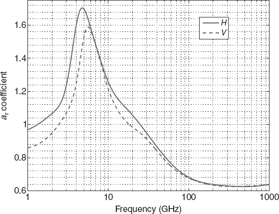
FIGURE 5.9 ar coefficients versus frequency for computing rain specific attenuation.

FIGURE 5.10 Rain specific attenuation versus frequency for selected rain rates.
given kH, kV, aH, and aV from the figures for horizontal and vertical polarizations. Here, θ represents the path elevation angle (with respect to the horizontal) of interest and τ is the polarization tilt angle with respect to horizontal (45° for circular). Note that the phase relationship between the vertical and horizontal field components is not relevant. Figure 5.10 plots rain specific attenuations versus frequency using these equations for a few rain rates and shows the importance of rain attenuation at frequencies greater than approximately 5 GHz.
5.4.4 Computing the Total Path Attenuation Through Rain
As with atmospheric gases, computing the total attenuation (in dB) of rain along a specified path requires integrating the specific attenuation (in dB per km) over the path length. For atmospheric gases, only vertical path variations were important because it could be assumed that the atmospheric composition is uniform horizontally, so that equation (5.23) applied. However, this is not true for rain, and both vertical and horizontal variations of the specific attenuation (or the rain rate) along the path must be considered. In general, it is quite difficult to describe horizontal and vertical variations of the rain rate that are applicable to a wide range of conditions, even at a fixed location. A useful quantity in this process is the “zero degree isotherm height” or “freezing height”, hR, which is the altitude at which the atmospheric temperature falls below freezing. Because ice causes much less attenuation than rain, rain attenuation can usually be neglected for portions of paths having altitudes greater than hR.
The freezing height is a meteorological parameter and therefore varies with season, location, and so on. ITU-R Recommendation P.839-3 [9] provides global maps of expected hR values. An approximation for hR that is useful over many global land areas is
where hR is in km and |ϕ| is the absolute value of the location latitude in degrees. This approximation shows that the freezing height ranges from approximately 5 km at the equator to near 0 km at the poles.
Even given a prediction for hR, a description of the vertical and horizontal variations of the rain rate is required to compute the total attenuation over a specific path. While studies that propose descriptions of rain rate spatial properties are not uncommon, their predictions are limited in applicability due to the difficulty in obtaining sufficient data on rain properties.
Consequently, empirical methods are the most practical approach for determining the total rain attenuation. Numerous empirical studies have been performed by placing a transmission of known transmit power (called a “beacon”) on either satellite or ground station platforms, and recording over a long time period (usually at least several years) the power received from this beacon in conjunction with local rain rates. Investigators across the globe have performed measurements of this sort since the 1960s, and an extensive database of measurements is available for developing empirical models.
Two methods are commonly used to represent empirical path attenuation information. In the first, the total attenuation along a path is described as the specific attenuation at ground level multiplied by an effective path length:
where Rr is the rain rate at ground level and LE is the effective path length that is determined from empirical Lrain,db measurements. An alternate approach uses
where ![]() or
or ![]() are effective specific attenuations or rain rates, respectively, that when multiplied by the true path length Ltrue yield the measured Lrain,db data. The true path length Ltrue is computed as the path distance between the station and the freezing height.
are effective specific attenuations or rain rates, respectively, that when multiplied by the true path length Ltrue yield the measured Lrain,db data. The true path length Ltrue is computed as the path distance between the station and the freezing height.
A significant number of descriptions of both LE and of ![]() have been proposed. The ITU-R continues to examine and cross-compare such models, but at present recommends in ITU-R P.618-9 [7] an approach (given below) that should provide rain attenuation predictions (in decibels) accurate to within approximately 20% on Earth to satellite paths. The ITU-R also specifies 20% as the expected variability in the rain attenuation from year to year.
have been proposed. The ITU-R continues to examine and cross-compare such models, but at present recommends in ITU-R P.618-9 [7] an approach (given below) that should provide rain attenuation predictions (in decibels) accurate to within approximately 20% on Earth to satellite paths. The ITU-R also specifies 20% as the expected variability in the rain attenuation from year to year.
The following ITU-R model is recommended for use on a global basis at frequencies up to 55 GHz; however, given the wide variations in meteorology that occur globally, it is unlikely that a globally averaged model will yield high accuracy for all locations. For this reason, it is almost always preferable to use local attenuation data if they are available when forecasting propagation behaviors, even if at a different frequency or polarization: methods for “scaling” such data sets to other frequencies and polarizations exist as will be described later. In the absence of such information, the following approach can be used.
5.4.4.1 ITU Model for Earth to Satellite Rain Attenuation Given the surface rain rate that is exceeded 0.01% of the time (Rr,0.01) at a ground station of height hS km above sea level, and a path elevation angle θ, the path length below the rain height is

where Re is the effective Earth radius 8500 km (as will be discussed further in Chapter 6); the lower equation accounts for refraction effects in the Earth's atmosphere at small elevation angles, which will also be discussed further in Chapter 6. The projection of LS onto the Earth's surface is also used:
Note if hS > hR, the predicted rain attenuation is zero.
The effective path length LE is specified as a product of two factors
The computation of LR, the modified true path length, involves the following steps:
- First compute the “horizontal reduction factor” r0.01:
where
 is the specific attenuation exceeded 0.01% of the time at ground level. The factor r0.01 is defined so that r0.01 LG can be interpreted as an estimate of the horizontal extent of the rain cell.
 - Next an angle ζ is computed as
- LR is then specified depending on ζ:
The above equations ensure that the modified true path length is always less than or equal to the original LS.


The computation of V0.01, which scales the modified true path length into the effective path length LE, involves the following steps:


Figure 5.11 illustrates LE under this model for varying frequency, path elevation angle, rain rate exceeded 0.01% of the time, and station latitude parameters, assuming a station height of 0 km and circular polarization. Figure 5.11a (for a vertical path and for station latitude 40°) shows that the effective path length increases as a function of frequency: this is due to the use of the surface rain rate in the computation, so that LE must vary with frequency to account for vertical variations in the local specific attenuation. In Figure 5.11a, the lower rain rates exceeded 0.01% of the time pertain to drier climates. Thunderstorms are rare in such climates; the rain is usually from stratiform clouds that extend over relatively large distances; hence the LE values are greater for such climates.

FIGURE 5.11 Earth to satellite effective path length for computing rain attenuation for various path elevation angle (θ), frequency, rain rate exceeded 0.01% of the time, and station latitude (ϕ) parameters.
Figure 5.11b (at frequency 35 GHz and station latitude 40°) illustrates the dependence of the effective path length on the elevation angle. The true path length LS is also included for comparison. The results show that the effective path length varies substantially from LS at low elevations, with greater LE values again obtained for drier climates.
Figure 5.11c considers the impact of the station latitude for three rain rates that are exceeded 0.01% of the time for vertical paths at 35 GHz. LE decreases significantly at higher latitudes primarily due to the decreased freezing height at such latitudes.
Figure 5.11d considers variations in LE with the rain rate that is exceeded 0.01% of the time for three frequencies; all curves show a decreasing trend of LE with that rain rate. The decrease is more rapid at lower frequencies.
Combined, these plots show an effective path length ranging from 0 to 8 km on vertical paths; these path lengths increase dramatically at lower elevation angles as seen in Figure 5.11b.
5.4.4.2 ITU-R Model for Rain Attenuation Between Earth Stations For links between two Earth stations, the effective path length LE to be used in equation (5.35) is specified in ITU-R P. 530-12 [10] as

where d is the path distance in km and

with Rr,0.01 in mm/h. The quantity d0 is an average horizontal extent of the rain and decreases from 35 km at low rain rates to 7.81 km at very high rain rates.
LE in equation (5.46) ranges from d when the path distance is much less than d0 (so that the entire path length is multiplied by the ground level αrain,db) to d0 when the path length is much larger than d0, so that rain attenuation is included only in the raining region.
5.4.5 Attenuation Statistics
The preceding discussions provide an effective path length that can be used to obtain an estimate of total path attenuation using ![]() . Given the use of Rr,0.01 (the surface rain rate exceeded 0.01% of the time for the ground station location) in the computations, the predicted attenuation Lrain,0.01 is the rain attenuation (in dB) that is expected to be exceeded 0.01% of the time. Since the ITU-R model for LE can be used only for Lrain,0.01, the expected attenuation exceeded in other percentiles must be determined through an additional procedure. The ITU-R recommends that the rain attenuation exceeded at other probabilities be determined directly from Lrain,0.01 by a “probability scaling” method. The recommended procedures are described in ITU-R P.618-9 [7] for Earth–space paths and in ITU-R P.530-12 [10] for ground-to-ground paths. Given Lrain,0.01, the rain attenuation exceeded p percent of the time, Lrain,p, on Earth–space paths is obtained from
. Given the use of Rr,0.01 (the surface rain rate exceeded 0.01% of the time for the ground station location) in the computations, the predicted attenuation Lrain,0.01 is the rain attenuation (in dB) that is expected to be exceeded 0.01% of the time. Since the ITU-R model for LE can be used only for Lrain,0.01, the expected attenuation exceeded in other percentiles must be determined through an additional procedure. The ITU-R recommends that the rain attenuation exceeded at other probabilities be determined directly from Lrain,0.01 by a “probability scaling” method. The recommended procedures are described in ITU-R P.618-9 [7] for Earth–space paths and in ITU-R P.530-12 [10] for ground-to-ground paths. Given Lrain,0.01, the rain attenuation exceeded p percent of the time, Lrain,p, on Earth–space paths is obtained from
where

This approach is specified as accurate for p ranging from 0.001% to 5%.
For ground-to-ground paths and for p ranging from 0.001% to 1%, the probability scaling equations are

Using these equations the rain attenuations exceeded at a specified percentage of the time can be determined; this makes it possible to produce rain rate attenuation distribution plots as in Figure 5.5. This approach assumes that the probability of exceeding a given surface rain rate versus the rain rate has a similar functional form in all global regions; again local information on attenuation statistics is preferred, if available, to this globally averaged approach.
5.4.6 Frequency Scaling
In some cases, local information on rain attenuation may be available at one frequency, but information is sought on an alternate nearby frequency. ITU-R P. 618-9 [7] states that for otherwise identical situations, for frequencies from 7 to 55 GHz, and at the same probability,

where Lrain,p(f1) is the known rain attenuation exceeded p percent of the time at frequency f1, and Lrain,p(f2) is the desired rain attenuation exceeded p percent of the time at frequency f2. In this equation,

and

5.4.7 Rain Margin Calculations: An Example
Consider a 12 GHz Earth to satellite link with the ground station location near Columbus, OH (latitude ≈ 40°, station height 0 km). The satellite is in a geostationary orbit (see appendix to this chapter) and is observed at range 38,000 km from the ground station at elevation angle 40°. Suppose the satellite transmitter transmits 120 W of power in a 24 MHz bandwidth using circular polarization and has an antenna gain of 46 dBi, while the receiver has a noise figure of 6 dB and the receive antenna gain is 30 dBi. The signal-to-noise ratio required for the system to function is 10 dB. Our goal is to assess the number of hours per year (on average) that the system would be expected to fail due to insufficient signal-to-noise ratio. It will be assumed throughout that the systems are impedance and polarization matched and that the antennas are directed to achieve maximum received power.
We begin by using the Friis formula to compute the signal-to-noise ratio neglecting atmospheric gas and rain attenuation:

while the thermal noise power level at the receiver (assuming a 290K external noise temperature) is

or −124.1 dBW. The signal-to-noise ratio achieved by neglecting rain and gas attenuation is then 15.3 dB, so 5.3 dB margin is achieved over the 10 dB signal-to-noise threshold required for operation.
Examination of Figure 5.3 shows the zenith gas attenuation through the entire atmosphere to be approximately 0.06 dB, so the slant path attenuation is estimated as 0.06 csc 40° = 0.09 dB. Gas attenuation at 12 GHz is generally negligible.
To investigate rain attenuation effects, begin by using Figure 5.7 to determine that the rain rate exceeded 0.01% of the time near Columbus, OH, is approximately 45 mm/h. Also, use Figures 5.8 and 5.9 to determine the appropriate kr values (0.024, 0.024) and ar values (1.12, 1.18) for vertical and horizontal polarizations, respectively, and equation (5.32) to determine kr and ar values of 0.024 and 1.15, respectively, for circular polarization (θ = 40°, τ = 45°).

FIGURE 5.12 Rain attenuation distribution function obtained in example problem.
The procedure of Section 5.4.4.1 is next applied to determine LE = 3.93 km, so the attenuation in decibels exceeded 0.01% of time is
Attenuations exceeded at other percentages of the time can be determined using the probability scaling approach of equation (5.48).
Unfortunately, equation (5.48) is not easy to invert to determine the percentage of time given a specific attenuation level, as we are seeking here. Instead, a graphical procedure can be used by plotting the predictions of equation (5.48) as shown in Figure 5.12. From the plot, we find that greater than 5.3 dB of rain attenuation occurs approximately 0.025% of the time, or approximately 2.2 h per year, on the average. If this level of reliability is not acceptable, additional transmit power could be added or other system properties modified in order to improve performance.
5.4.8 Site Diversity Improvements
Given the large effect that rain attenuation can have on system reliability, especially at higher frequencies, methods for overcoming these effects are sometimes necessary if reliable links are to be obtained. “Site diversity” refers to the use of multiple antennas that are separated by appreciable distances for signal reception, with some method of choosing or combining the multiple signals received to improve the performance over that of a single antenna. Site diversity should be expected to yield system improvements because the large rain rates that lead to the largest attenuations often have rather small horizontal extents, so another antenna located outside of the rain cell would have a greatly reduced attenuation.

FIGURE 5.13 Hypothetical rain attenuation distributions and diversity effects.
Figure 5.13 illustrates two hypothetical rain attenuation distributions obtained for a single antenna and a diversity system. The single antenna curve shows attenuations greater than 40 dB for more than 0.01% of the time. However, the diversity or “two-antenna” curve shows better performance, with less than 30 dB attenuation exceeded 0.01% of the time. The “diversity gain” obtained is defined as Gd in the figure and is the difference between attenuations (in decibels) in the single antenna and diversity systems for a specified probability. The “diversity improvement” is labeled I in the figure, and is defined as the ratio of the probabilities for a specified attenuation.
An important issue in diversity systems is the method that is chosen for combining the signals from different antennas. An approach that is sometimes applied is to switch in a binary fashion to the signal receiving the most power, in which case the diversity system output is that of the antenna with higher power. However, this approach can require rapid switching between systems and becomes impractical at higher data rates. A second approach is to always combine signals from different antennas in a ratio proportional to their signal-to-noise ratios.
Of course, the expected improvement of a diversity system depends strongly on the distance separating the antennas—a zero separation would clearly not yield any improvement! Figure 5.14 plots the two-antenna diversity gain versus separation distance as described in ITU-R Recommendation P.618-9 [7]. The different curves on this plot were obtained for varying rain attenuations (or “fade depths”) in the worst antenna (indicated in the figure legend) and illustrate that diversity gain is also clearly associated with the fade strength observed. Note that the most improvement is obtained in the highest fade situations, which should be expected since it is here that rain attenuation is playing the major role. The saturation in these curves as distance increases gives some idea of the typical horizontal extent of a rain event, with a separation of 8 km clearly larger than the extent of the more significant rain events observed.

FIGURE 5.14 Sample plots of diversity gain versus separation distance.
ITU-R Recommendation P.618-9 provides an empirical model of the diversity gain Gd in dB as
The site separation factor, Gs is
where d is the antenna separation in km and
and A is the single-site rain attenuation in dB. The frequency factor Gf is
The elevation factor Gθ is
where θ is the elevation angle in degrees, and the baseline orientation factor Gδ is
where δ is the acute angle between the great circle connecting the two stations and the projection onto the Earth surface of the path to the satellite from one of the stations, in degrees.
A more accurate method for predicting the outage probability due to rain attenuation in a system with two-antenna site diversity is also given in ITU-R P.618-9; this method however is more complex and provides less physical insight than the simpler approach presented above.
Amodel for the diversity improvement is also provided in earlier versions of ITU-R P.618 as

where
and where d is again the antenna separation in km. Here, p1 and p2 refer to the percentages of time that a given rain attenuation is observed for the one- and two-antenna cases, respectively. It is interesting to note that, unlike the diversity gain, the diversity improvement is modeled as independent of the rain attenuation level.
5.5 SCINTILLATIONS
Scintillation on a radiowave path is the name given to rapid fluctuations of the amplitude, phase, or angle of arrival of the wave passing through a medium with small-scale dielectric constant irregularities that cause changes in the transmission path with time. Scintillation effects, sometimes also referred to as atmospheric multipath fading, can be produced in both the troposphere and the ionosphere, with the major ionospheric effects occurring at frequencies below 2 GHz (ionospheric scintillations will be discussed in Chapter 11). To a first approximation, the dielectric constant structure can be considered as horizontally stratified, and variations appear as thin layers that change with altitude. Slant paths at low elevation angles tend to be affected most by scintillation conditions. Tropospheric scintillation is typically produced in the first few kilometers of altitude by high humidity gradients and temperature inversion layers. The effects are seasonally dependent and vary from day to day, as well as with the local climate.
Extensive observations of amplitude scintillations have been performed, and ITU-R Recommendation 618-9 [7] provides an empirical attenuation distribution for tropospheric attenuation caused by scintillation effects. Generally, frequencies from 2 to 20 GHz show scintillations less than 0.5–1 dB at high elevation angles (from 20° to 30°) in a temperate climate. Information on the expected rates of fading is also included in Recommendation 618 and shows that both “fast” (i.e., <1 s) and slow (periods of 10 s or more) fading components can occur, with the latter more important at low elevation angles. At lower frequencies, scintillations in the ionosphere must also be considered.
The measurements show a very definite increase in the magnitude of scintillation effects as the elevation angle is reduced below 10°. Deep fades of 20 dB or more with a few seconds duration have been observed; such fades are indicative of multipath contributions to scintillation effects. Multipath fading mechanisms will be discussed in more detail in Chapter 8. In some cases, scintillation effects can be attributed to variations in the angle of arrival of the signal transmitted from a satellite; to a high-gain receiving antenna, such variations in the angle of arrival cause variations in the received power, and therefore appear to be amplitude variations.
It is important to be aware of potential atmospheric scintillation effects, especially at lower elevation angles, so that they will not be confused with system errors or system noise!
APPENDIX 5.A LOOK ANGLES TO GEOSTATIONARY SATELLITES
Since our methods for predicting propagation under direct transmission conditions are frequently applied to satellite systems, it is useful to have a method for computing the elevation and azimuth angles at which a satellite appears to the Earth station. For example, if the Earth station receives the satellite signal, then these angles are the θR, ϕR of equations (5.3) and (5.5).
When a satellite is injected into a circular orbit 35,900 km (22,300 miles) above the surface of the Earth, its period equals that of the Earth's rotation. If the orbit is in the Earth's equatorial plane, the satellite will rotate in synchronism with the Earth and appear to be stationary. Such “geostationary” satellites are very useful for communications because Earth station antennas do not need elaborate steering mechanisms to track the satellites. In practice, complete stationarity is not realized because the Earth is not a homogeneous sphere, and the satellite orbit is affected by the gravitational anomalies that exist. As a result, satellites in geostationary orbits appear to drift in a small diurnal pattern, generally subtending a small fraction of a degree of arc from an Earth station, so that low-gain antennas often need not be steered at all, while the tracking requirements of high-gain antennas are minimized. Of course, geostationary orbits are not the only possible satellite orbits! We will limit ourselves to this situation only for simplicity.
Earth stations communicating with satellites in geostationary orbits need to be able to orient antennas in the proper direction, specified by the elevation and azimuth angles to the satellite. A derivation of these angles based on the latitude and longitude of the Earth station and subsatellite points on the Earth's surface (the point on the Earth's surface on a line between the center of the Earth and the satellite) is as follows: For an Earth station located at point B (latitude θ′, longitude ϕ′) and subsatellite point A (latitude 0°, longitude ϕ0), as shown in Figure 5.15, spherical trigonometry shows

FIGURE 5.15 Geometry for defining look angles.
The azimuth bearing of the satellite as seen from a station in the Northern hemisphere is therefore π + β for a satellite west of the station and π − β for a satellite east of the station.
For a station in the Southern hemisphere, the corresponding relations are
and the azimuth bearing is 2π − β for a satellite west of the station and β for a satellite to the east of the station.
In Figure 5.16, the plane of the page is determined by the subsatellite point A, the station location B, and the center of the Earth O. Since A is the intersection of OS with the Earth surface, S is also in the plane of the page. The central angle δ measures the great-circle arc AB, as implied by Figure 5.15. Applying the law of cosines to the plane triangle OBS gives

FIGURE 5.16 Geometry for finding elevation angle.
The distance CB is given by
and also by
Equating the previous two equations allows solution for the elevation angle Δ as
which is valid for both the Northern and Southern hemispheres.
REFERENCES
1. ITU-R Recommendation P.676-7, “Attenuation by atmospheric gases,” International Telecommunication Union, 2007.
2. ITU-R Recommendation P.840-3, “Attenuation due to clouds and fog,” International Telecommunication Union, 1999.
3. Marshall, J. S. and W. M. K. Palmer, “The distribution of raindrops with size,” J. Meteor., vol. 5, pp. 165–166, 1948.
4. Williams, C. R. and K. S. Gage, “Raindrop size distribution variability estimated using ensemble statistics,” Ann. Geophys., vol. 27, pp. 555–567, 2009.
5. ITU-R Recommendation P.837-5, “Characteristics of precipitation for propagation modeling,” International Telecommunication Union, 2007.
6. Van de Hulst, H. C., Light Scattering by Small Particles, Dover Publications, 1981.
7. ITU-R Recommendation P.618-9, “Propagation data and prediction methods required for the design of Earth–space telecommunication systems,” International Telecommunication Union, 2007.
8. ITU-R Recommendation P.838-3, “Specific attenuation model for rain for use in prediction methods,” International Telecommunication Union, 2005.
9. ITU-R Recommendation P.839-3, “Rain height model for prediction methods,” International Telecommunication Union, 2001.
10. ITU-R Recommendation P.530-12, “Propagation data and prediction methods required for the design of terrestrial line-of-sight systems,” International Telecommunication Union, 2007.
Radiowave Propagation: Physics and Applications. By Curt A. Levis, Joel T. Johnson, and Fernando L. Teixeira
Copyright © 2010 John Wiley & Sons, Inc.