
6
REFLECTION AND REFRACTION
6.1 INTRODUCTION
In many situations, Earth terrain and/or the atmosphere may be modeled as consisting of layers of dielectric media separated by planar or spherical interfaces. Analytical models for such configurations are well established [1–3]: the basic formalisms of reflection and refraction for a planar boundary are reviewed in this chapter to prepare for their application to path loss predictions in subsequent chapters. The basic theory of refraction derived in this chapter is also applied to study the propagation of electromagnetic waves in an inhomogeneous atmosphere above a spherical Earth, and the ducting phenomena that can result are investigated.
6.2 REFLECTION FROM A PLANAR INTERFACE: NORMAL INCIDENCE
Consider an interface between two linear, homogeneous, isotropic, and time-invariant media located in the xy plane as shown in Figure 6.1. Regions 1 and 2 are located above and below the interface, respectively, and are characterized by ∈i, μi, and σi where i = 1, 2. Our experience tells us that a wave that encounters a boundary with a different medium will have some portion of its energy reflected from the boundary while the remainder is transmitted; for example, in a piece of glass one can see both reflected light (forming an image of the observer) and light transmitted from the other side. A determination of how much energy is reflected given the properties of the two media, however, requires use of electromagnetic theory and is considered in this section for a plane wave propagating in a direction normal to the interface. In this case, an azimuthal symmetry exists about the z axis since the interface is a plane. Thus, the final solution to the problem should have no dependence on the x or y coordinates, and the resulting reflected and transmitted fields should have the same amplitude regardless of their polarization.

FIGURE 6.1 Geometry for normal incidence reflection.
To represent a general linear polarization, let us choose the incident electric field to be polarized in the ![]() direction. Propagation in the −
direction. Propagation in the −![]() direction then implies that the incident magnetic field is in the
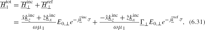
direction then implies that the incident magnetic field is in the ![]() direction. As stated previously, a reflected plane wave should result in region 1 while a transmitted plane wave results in region 2. The total electric and magnetic fields in regions 1 and 2 can then be written as
direction. As stated previously, a reflected plane wave should result in region 1 while a transmitted plane wave results in region 2. The total electric and magnetic fields in regions 1 and 2 can then be written as
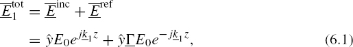
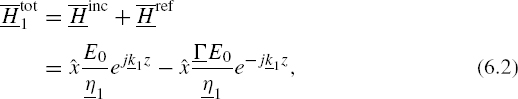
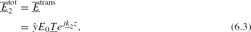

where E0 is an arbitrary amplitude, and the propagation constant of plane waves in different dielectric media has been incorporated through ![]()
![]() . The appropriate propagation and field polarization directions are indicated. The field polarization directions result from the fact that Maxwell's equations dictate that tangential electric and magnetic fields must be continuous at a sourceless dielectric interface. Since the incident electric field is polarized in the
. The appropriate propagation and field polarization directions are indicated. The field polarization directions result from the fact that Maxwell's equations dictate that tangential electric and magnetic fields must be continuous at a sourceless dielectric interface. Since the incident electric field is polarized in the ![]() direction, reflected and transmitted electric fields must also be polarized in this same direction if tangential
direction, reflected and transmitted electric fields must also be polarized in this same direction if tangential ![]() fields are to be continuous. The coefficients Γ and T in the above equations represent the reflected and transmitted electric field amplitudes relative to the incident wave amplitude E0, and are known as the Fresnel reflection and transmission coefficients, respectively. These coefficients are as yet unknown, but applying the boundary conditions to equations (6.1)–(6.4) will enable them to be determined.
fields are to be continuous. The coefficients Γ and T in the above equations represent the reflected and transmitted electric field amplitudes relative to the incident wave amplitude E0, and are known as the Fresnel reflection and transmission coefficients, respectively. These coefficients are as yet unknown, but applying the boundary conditions to equations (6.1)–(6.4) will enable them to be determined.
Matching tangential electric fields (the entire electric field in this case since ![]() is tangential to the boundary) at the boundary z = 0 from equations (6.1) and (6.3) yields
is tangential to the boundary) at the boundary z = 0 from equations (6.1) and (6.3) yields
while matching tangential magnetic fields from equations (6.2) and (6.4) yields

Solving these two equations yields


An examination of equation (6.7) shows that no reflected wave will be produced (i.e., Γ = 0) if ![]() , that is,
, that is, ![]() . While this equation is true if we have the same medium on both sides of the boundary, that is,
. While this equation is true if we have the same medium on both sides of the boundary, that is, ![]() as one would expect, no reflected wave can be obtained if there are different media on both sides of the boundary but the intrinsic impedances are equal (requires magnetic materials).
as one would expect, no reflected wave can be obtained if there are different media on both sides of the boundary but the intrinsic impedances are equal (requires magnetic materials).
Also note that the Γ derived in equation (6.7) is an electric field reflection coefficient, so the reflected power density relative to the incident power density is ![]() .
.
6.3 REFLECTION FROM A PLANAR INTERFACE: OBLIQUE INCIDENCE
The reflection problem becomes more involved if the incident field is not propagating in a direction normal to the boundary because the azimuthal symmetry is lost in this case, so that the problem is no longer invariant with respect to incident field polarization. In general, any electromagnetic wave can be written as the sum of two orthogonal field components in a plane normal to the direction of propagation. Since Maxwell's equations are linear, the reflection problem can be solved separately for each of these two field components, and then the solution for a wave having any polarization can be written as the sum of the two component solutions multiplied by the corresponding component amplitudes of the specified incident wave.
6.3.1 Plane of Incidence
The standard choice for the two field polarization components for which we will solve the reflection problem involves the “plane of incidence,” defined to be a plane containing both the incident field propagation direction and the normal to the surface. The plane of incidence is the plane that is usually drawn when considering oblique incidence reflection problems, as shown in Figure 6.2; that is, the plane of the page is the plane of incidence for this figure. Clearly, any arbitrary field polarization can be written as the sum of one component that is parallel to the plane of incidence and perpendicular to the propagation direction and a second component that is perpendicular to the plane of incidence (i.e., pointing in the ![]() direction into the page.) Standard notation defines a field as having parallel polarization if its electric field vector lies in the plane of incidence, and perpendicular polarization if its electric field vector is perpendicular to the plane of incidence. These two polarizations are also called vertical and horizontal, respectively, in problems where the boundary represents a horizontal plane such as the ground, or TM and TE, for transverse magnetic or transverse electric, respectively, depending on which field component is perpendicular to the plane of incidence.
direction into the page.) Standard notation defines a field as having parallel polarization if its electric field vector lies in the plane of incidence, and perpendicular polarization if its electric field vector is perpendicular to the plane of incidence. These two polarizations are also called vertical and horizontal, respectively, in problems where the boundary represents a horizontal plane such as the ground, or TM and TE, for transverse magnetic or transverse electric, respectively, depending on which field component is perpendicular to the plane of incidence.

FIGURE 6.2 Geometry for oblique incidence reflection: perpendicular polarization.
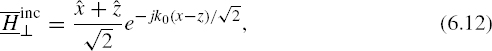
As an example of representing an arbitrarily polarized wave in terms of its parallel and perpendicular polarization components, consider the following incident field propagating in the ![]() direction from free space onto a “horizontal” boundary in the xy plane:
direction from free space onto a “horizontal” boundary in the xy plane:

The first two components of ![]() are “horizontal,” so one may be tempted to take them and the associated magnetic field as the perpendicular (or horizontal) polarized electric field component. Similarly, the first two components of
are “horizontal,” so one may be tempted to take them and the associated magnetic field as the perpendicular (or horizontal) polarized electric field component. Similarly, the first two components of ![]() are “horizontal,” so one might be tempted to take them and the associated electric field as being parallel (or vertical) polarization. Such a decomposition is not useful because the decomposed fields are not transverse to the direction of propagation and therefore do not correspond to solutions of Maxwell's equations in this problem.
are “horizontal,” so one might be tempted to take them and the associated electric field as being parallel (or vertical) polarization. Such a decomposition is not useful because the decomposed fields are not transverse to the direction of propagation and therefore do not correspond to solutions of Maxwell's equations in this problem.
The correct way to decompose the field is to use the plane of incidence defined by ![]() , that is, a plane normal to the −
, that is, a plane normal to the −![]() direction or the xz plane. Then the perpendicular (therefore horizontal) polarized field is
direction or the xz plane. Then the perpendicular (therefore horizontal) polarized field is
and the associated magnetic field is
while the parallel polarized fields are

We now proceed to solve the reflection problem, beginning with perpendicular polarization.
6.3.2 Perpendicular Polarized Fields in Regions 1 and 2
In the perpendicular polarized case, the electric field vector is polarized perpendicular to the plane of incidence, that is, in the ![]() direction in Figure 6.2. Defining θi, θr and θt as the angles between the z axis and the propagation directions (as shown in Figure 6.2) allows the incident, reflected, and transmitted
direction in Figure 6.2. Defining θi, θr and θt as the angles between the z axis and the propagation directions (as shown in Figure 6.2) allows the incident, reflected, and transmitted ![]() vectors to be written, respectively, as
vectors to be written, respectively, as
where the fact that
has been used. Note that θr and θt are as yet unknown. A consideration of the boundary conditions results in a “phase matching” condition that will enable these angles to be determined.
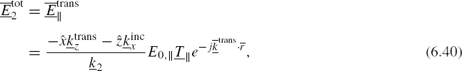
Total electric fields in regions 1 and 2 can then be written as


and their associated magnetic fields derived from equation (3.26). Again, the ![]() polarization assumed for the reflected and transmitted waves reflects the fact that the boundary conditions require tangential electric fields to be continuous, so that the sole
polarization assumed for the reflected and transmitted waves reflects the fact that the boundary conditions require tangential electric fields to be continuous, so that the sole ![]() component of the incident fields dictates that the reflected and transmitted fields also have only a
component of the incident fields dictates that the reflected and transmitted fields also have only a ![]() component.
component.
6.3.3 Phase Matching and Snell's Law
The boundary conditions for reflection from a boundary between two dielectric media require that tangential electric and magnetic field components are continuous at the boundary; that is, that the same value of the field is approached as one moves toward the boundary from either side. Examining the incident electric field for this oblique incidence case shows that there is a phase variation along the boundary (i.e., the plane z = 0), given by
If total tangential fields at the boundary are to be continuous, it is clear that reflected and transmitted fields must retain this same phase variation. Thus, the x components of the ![]() vectors must be the same for the incident, reflected, and transmitted waves, or more generally, the components of the
vectors must be the same for the incident, reflected, and transmitted waves, or more generally, the components of the ![]() vectors tangential to the boundary must be the same. This requirement is known as the “phase matching” condition.
vectors tangential to the boundary must be the same. This requirement is known as the “phase matching” condition.
Phase matching has some immediate consequences in terms of the reflected and transmitted wave propagation directions. For the reflected wave, phase matching requires ![]() , which from equations (6.15) and (6.16) implies θr = θi. This is known as the “law of reflection.”
, which from equations (6.15) and (6.16) implies θr = θi. This is known as the “law of reflection.”
Phase matching also allows the direction of the transmitted wave to be determined. Beginning with the transmitted ![]() vector
vector
phase matching requires
while equation (6.19) states that
Equations (6.24) and (6.25) can then be used to obtain
allowing both components of the transmitted ![]() vector to be determined once
vector to be determined once ![]() and the medium properties are known. When both media are lossless (i.e., σi = 0) and clear propagation angles exist, this relationship is known as “Snell's law.” In this case,
and the medium properties are known. When both media are lossless (i.e., σi = 0) and clear propagation angles exist, this relationship is known as “Snell's law.” In this case, ![]() and
and ![]() , yielding
, yielding

which is a more typical form for Snell's law. Equation (6.28) shows that when propagating from a less dense into a more dense medium, that is, ![]() , the transmitted angle is smaller than the incident angle, that is, sin θt < sin θi, indicating that the wave propagates along a direction closer to the normal. Conversely, when a wave propagates from a more dense to a less dense medium, sin θt > sin θi and the transmitted wave is bent away from the normal. This bending of the rays is known as refraction. With nonmagnetic media on both sides of the boundary, Snell's law reduces to
, the transmitted angle is smaller than the incident angle, that is, sin θt < sin θi, indicating that the wave propagates along a direction closer to the normal. Conversely, when a wave propagates from a more dense to a less dense medium, sin θt > sin θi and the transmitted wave is bent away from the normal. This bending of the rays is known as refraction. With nonmagnetic media on both sides of the boundary, Snell's law reduces to
or simply
where ni is the index of refraction or refractive index, given by ![]() in nonmagnetic media). Refraction has important consequences for propagation through the Earth's atmosphere and will be discussed in more detail later in this chapter.
in nonmagnetic media). Refraction has important consequences for propagation through the Earth's atmosphere and will be discussed in more detail later in this chapter.
6.3.4 Perpendicular Reflection Coefficient
Now that the components of the ![]() vectors have been determined, total magnetic fields in regions 1 and 2 can be written and the boundary conditions applied to determined
vectors have been determined, total magnetic fields in regions 1 and 2 can be written and the boundary conditions applied to determined ![]() and
and ![]() . Using the fact that
. Using the fact that ![]() , we obtain
, we obtain

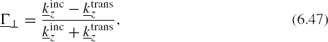
Setting tangential electric and magnetic fields equal at z = 0 yields

where only the x component of the magnetic field has been used since the z component is not tangential to the boundary. Solving these two equations yields


Sometimes it is useful to consider oblique incidence on a perfectly conducting medium. As in the case of normal incidence, one finds ![]() , and there is no transmission into the perfectly conducting medium as the magnetic field is terminated by a surface current.
, and there is no transmission into the perfectly conducting medium as the magnetic field is terminated by a surface current.
This concludes the solution for the perpendicular polarized case. Note that again the fraction of power density reflected is ![]() .
.
6.3.5 Parallel Polarized Fields in Regions 1 and 2
In the parallel polarized case, the electric field vector is polarized in the plane of incidence, as shown in Figure 6.3, which requires the magnetic field vector to be polarized perpendicular to the plane of incidence. In this case, it is easier to begin with the magnetic fields since they have only a ![]() component. Total magnetic fields in regions 1 and 2 analogous to equations (6.20)–(6.21) can be written as
component. Total magnetic fields in regions 1 and 2 analogous to equations (6.20)–(6.21) can be written as

FIGURE 6.3 Geometry for oblique incidence reflection: parallel polarization.


Since the boundary conditions are the same as in the perpendicular polarization case, the phase matching condition still holds and the incident, reflected, and transmitted ![]() vectors are the same as those of the previous section, so that Snell's law (6.28) holds also for parallel polarization for lossless media. Electric fields for the parallel polarized case can be derived using
vectors are the same as those of the previous section, so that Snell's law (6.28) holds also for parallel polarization for lossless media. Electric fields for the parallel polarized case can be derived using ![]() to be
to be

where ![]() .
.
6.3.6 Parallel Reflection Coefficient
Setting tangential electric and magnetic fields equal at z = 0 yields
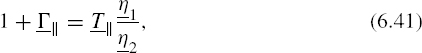

where only the x component of the electric field has been used since the z component is not tangential to the boundary. Solving these two equations yields


This concludes the solution for the parallel polarized case. Note that again the fraction of the power density reflected is ![]() . While the use of a reflection coefficient for the magnetic field for parallel polarization is convenient in the derivation, a reflection coefficient for the electric field is often used in the literature and will be used in Chapters 7 and 9. From (6.39), the reflected electric field tangential and normal components are
. While the use of a reflection coefficient for the magnetic field for parallel polarization is convenient in the derivation, a reflection coefficient for the electric field is often used in the literature and will be used in Chapters 7 and 9. From (6.39), the reflected electric field tangential and normal components are ![]() and
and ![]() , respectively, times the corresponding incident field components. The case of normal incidence can be treated as either parallel or perpendicular polarization, with the same result for the ratio of reflected to incident electric fields, even though
, respectively, times the corresponding incident field components. The case of normal incidence can be treated as either parallel or perpendicular polarization, with the same result for the ratio of reflected to incident electric fields, even though ![]() and
and ![]() are defined differently and differ by a minus sign in this limit.
are defined differently and differ by a minus sign in this limit.
6.3.7 Summary of Reflection Problem
The solutions we have obtained so far for the parallel and perpendicular polarization cases also enable the solution for any arbitrarily polarized incident field to be constructed. Returning to the example given in equations (6.9)–(6.14), we have

illustrating the decomposition of an arbitrarily polarized wave into its parallel and perpendicular components along with the determination of the appropriate field component amplitudes (the E0 values given in parenthesis) associated with a particular set of definitions in the problem solution. The reflected wave for this incident wave is then given by
where ![]() and
and ![]() are as specified in the rightmost terms of equations (6.20) and (6.39), respectively. Note that the reflection coefficients for perpendicular and parallel polarizations are usually not equal. As a result, the original polarization of the incident wave can be modified upon reflection.
are as specified in the rightmost terms of equations (6.20) and (6.39), respectively. Note that the reflection coefficients for perpendicular and parallel polarizations are usually not equal. As a result, the original polarization of the incident wave can be modified upon reflection.
The reflection coefficients derived can also be simplified for application to cases of particular interest. Noting that magnetic media are uncommon in typical propagation problems, we set μ2 = μ1 to obtain

Furthermore, using ![]() and
and ![]() from equation (6.26), we obtain
from equation (6.26), we obtain


Magnitudes of ![]() and
and ![]() are plotted versus θi for a boundary between free space and “wet ground” (Figure 2.5) in Figure 6.4 for three different frequencies. From these plots, it is apparent that
are plotted versus θi for a boundary between free space and “wet ground” (Figure 2.5) in Figure 6.4 for three different frequencies. From these plots, it is apparent that ![]() for all incidence angles when
for all incidence angles when ![]() , a fact that can be proven for all dielectric media from equations (6.49) and (6.50). It is also observed that the magnitude of both reflection coefficients approaches unity as θi approaches 90° (also known as “grazing incidence”).
, a fact that can be proven for all dielectric media from equations (6.49) and (6.50). It is also observed that the magnitude of both reflection coefficients approaches unity as θi approaches 90° (also known as “grazing incidence”).

FIGURE 6.4 Typical reflectivities at a boundary between free space and “wet ground” versus incidence angle.
An examination of equation (6.49) shows that ![]() can be obtained only if
can be obtained only if ![]() , in which case no reflection is expected. For
, in which case no reflection is expected. For ![]() , however, an equation
, however, an equation

is obtained, which can be solved for the “Brewster angle,” θB as

Thus, a parallel (or vertically) polarized wave will generate no reflected wave if it is incident at angle θB. Note that θB is a real angle only if ![]() and
and ![]() are purely real; that is, there is no loss in either region. However, a minimum reflection still exists in the lossy medium case near the “pseudo-Brewster angle” predicted by using
are purely real; that is, there is no loss in either region. However, a minimum reflection still exists in the lossy medium case near the “pseudo-Brewster angle” predicted by using ![]() in equation (6.52).
in equation (6.52).
The phases of ![]() and
and ![]() near grazing are also of importance. Equation (6.49) shows that
near grazing are also of importance. Equation (6.49) shows that ![]() approaches −1 at grazing, indicating a zero total tangential electric field on the boundary. The analysis of the behavior of
approaches −1 at grazing, indicating a zero total tangential electric field on the boundary. The analysis of the behavior of ![]() at grazing is not as immediately clear. The phase of
at grazing is not as immediately clear. The phase of ![]() near grazing depends on
near grazing depends on ![]() in (6.50), but it can be shown that
in (6.50), but it can be shown that ![]() also approaches −1 at near grazing angles. In fact, the phase of
also approaches −1 at near grazing angles. In fact, the phase of ![]() is positive for incidence angles less than the Brewster or pseudo-Brewster angle, but becomes negative once the incidence angle exceeds the Brewster angle.
is positive for incidence angles less than the Brewster or pseudo-Brewster angle, but becomes negative once the incidence angle exceeds the Brewster angle.
6.4 TOTAL REFLECTION AND CRITICAL ANGLE
We now return to a closer examination of an interesting consequence of Snell's law, given by equation (6.28) for the lossless medium case as

We have previously discerned that this equation predicts a transmitted wave traveling closer to the normal direction if propagation is from a less dense to a more dense medium, or a transmitted wave traveling further from the normal direction if propagation is from a more dense to a less dense medium. In the latter case some interesting phenomena can occur that reveal surprising solutions of Maxwell's equations that play an important role in wave propagation. Clearly, the problem with equation (6.53) in this case occurs when

because then there is no real-valued solution for sin θt. The angle when this first occurs is defined as the “critical angle,” θc, and is found by replacing the > sign with equality in equation (6.54) to obtain
What happens in the reflection problem at or beyond the critical angle? It is easier to examine these effects by returning to the phase matching condition ![]() and equation (6.26)
and equation (6.26)

which is seen from equation (6.54) to yield a negative value for ![]() when the critical angle is exceeded. This implies that
when the critical angle is exceeded. This implies that ![]() becomes imaginary in the transmitted medium, so that instead of propagating away from the boundary, the field decays exponentially. Note that we are still considering lossless media only, so that the resulting decay is not a consequence of a medium conductivity. Rather, this is another type of solution to Maxwell's equations, a wave that decays in a lossless medium. This type of solution is called an “evanescent wave.”
becomes imaginary in the transmitted medium, so that instead of propagating away from the boundary, the field decays exponentially. Note that we are still considering lossless media only, so that the resulting decay is not a consequence of a medium conductivity. Rather, this is another type of solution to Maxwell's equations, a wave that decays in a lossless medium. This type of solution is called an “evanescent wave.”
The reflection coefficients given by equations (6.35)

can also be simplified in this case because all elements in these equations are assumed to be real except for ![]() , which is purely imaginary when the critical angle is exceeded. Both of these reflection coefficients can then be written in the form
, which is purely imaginary when the critical angle is exceeded. Both of these reflection coefficients can then be written in the form
for which
which means that the wave is totally reflected. This phenomenon is known as “total reflection,” indicating that a wave incident from a more dense medium to a less dense medium beyond the critical angle will be completely reflected. A phase shift of ej2ϕ, known as the Goos–Hanchen phase shift, does result, however.
Let us now consider the form of the electric and magnetic fields in the transmitted medium. Defining ![]() , where α is a positive real number, to account for the imaginary component, transmitted fields for the perpendicular polarized case are
, where α is a positive real number, to account for the imaginary component, transmitted fields for the perpendicular polarized case are

Note that decay of the fields away from the boundary is expressed in these equations since in region 2, z becomes more negative as one moves away from the boundary. This type of evanescent wave is also referred to as a “surface wave” because of such properties; that is, the field is strongest near the surface and decreases as one moves away from the surface. An examination of equation (6.56) shows that we could also have chosen ![]() , where α is a positive real, since only
, where α is a positive real, since only ![]() is specified in equation (6.56). However, this choice would result in an increasing field amplitude as one moves away from the boundary that grows without bound since the transmitted medium is unbounded in the −z direction. Because this would require infinite energy, this choice is discarded as being nonphysical.
is specified in equation (6.56). However, this choice would result in an increasing field amplitude as one moves away from the boundary that grows without bound since the transmitted medium is unbounded in the −z direction. Because this would require infinite energy, this choice is discarded as being nonphysical.
The fact that the incident wave has undergone “total reflection” while a transmitted field still remains may cause some confusion. However, if the Poynting vector of the transmitted wave is calculated (peak value phasors), we obtain

showing that the surface wave carries power along the surface but that there is no power flow perpendicular to the surface in the steady state. Thus, an observer moving far away from the boundary in the (lossless) transmitted medium would measure no power at all, while an observer in the reflected medium would observe total power reflection. Of course, the creation of the evanescent field in the transmitted medium would originally require some power flow across the boundary in a transient state, but once the steady state is reached, the transmitted field is solely an energy storing field.
The surface wave in this reflection problem is of importance, but is not quite the same as the “surface wave” or “ground wave” typically discussed in propagation problems. However, the ground wave considered in Chapter 9 has properties similar to these evanescent waves. Hence, from this point forward, we should be aware that, in addition to the standard propagating wave solutions of Maxwell's equations, evanescent wave solutions are possible as well, with the sole requirement that
and no restriction otherwise on the complex components of the ![]() vector.
vector.
6.5 REFRACTION IN A STRATIFIED MEDIUM
Now that we have derived Snell's law for a single planar interface, we can consider refraction effects in a medium consisting of many planar interfaces, each individual interface with only slightly different dielectric constants so that reflections may be considered negligible. The basic configuration is shown in Figure 6.5 and consists of a series of nonmagnetic media having refractive indices (defined below equation (6.30)) n0, n1, …. A plane wave is incident on the boundary between layers 0 and 1 with incidence angle θ0. Note that since we are neglecting reflections in this problem and considering only refraction, the polarization of the incident wave is not of importance. Snell's law as stated in equation (6.30) at the boundary between layers 0 and 1 requires

FIGURE 6.5 Geometry of planar stratified medium.
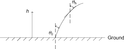
FIGURE 6.6 Variation in propagation angle with height.
In a similar manner, we can obtain at the boundary between layers 1 and 2
Combining (6.65) and (6.66), we obtain
and by continuing the same procedure, we can obtain for region r
A continuously horizontally stratified medium can be thought of as consisting of the limit of a discretely stratified medium as the layers become thinner and increase indefinitely in number, as shown in Figure 6.6. For such a medium, n becomes a continuous function of height, and therefore at any height h, the tangent to the ray of the propagating wave will have a direction given by
Our neglect of reflections requires that n(h) should vary slowly with respect to the electromagnetic wavelength in order to make reflections negligible.
6.6 REFRACTION OVER A SPHERICAL EARTH
The previous section considered refraction in a stratified, planar medium. However, propagation over the surface of the Earth requires consideration of the Earth's spherical shape: the Earth's atmosphere is stratified in spherical, rather than planar layers, as illustrated in Figure 6.7.
To derive the refraction properties of such a medium, we return again initially to a discretely stratified medium before considering the continuous case. For the discrete medium,

FIGURE 6.7 Geometry of spherically stratified medium.

From Figure 6.7, applying Snell's law at A results in
Figure 6.8 shows the region in the vicinity of AB of Figure 6.7 in more detail; also, a rectangle BDAC has been constructed using the fact that α1 is the angle with respect to the normal direction defined at point B. We find
where r0 is the radius of the Earth. Similarly, a rectangle AEBF can be defined as in Figure 6.9 using the fact that ![]() is the angle with respect to the normal direction defined at point A. Using this triangle, we find
is the angle with respect to the normal direction defined at point A. Using this triangle, we find
Therefore,

FIGURE 6.8 Detail of rectangle ABCD.
and substitution of this into (6.71) yields
which is Snell's law for a spherically stratified medium. In the same way, one can show
so that at all boundaries in the medium
is satisfied.

FIGURE 6.9 Detail of rectangle AEBF.

Media that vary continuously are more characteristic of nature than discretely layered media; again these can be viewed as the limiting case as the number of layers increases and the radial distances between layers decrease to zero. In this case, the limiting form of equation (6.77) becomes
With some exceptions, such as in communication links between aircraft and satellites or those involving ionosphere reflections, propagation paths generally occur relatively close to the Earth surface, and the angles α and α0 approach π/2 rad. It is then more convenient to use the complementary angles ψ and ψ0 (i.e., the “elevation angles”) shown in Figure 6.10 because they are small so that small-angle approximations can be used. Equation (6.78) then transforms to
Let the subscript 0 refer to the surface of the Earth. Then r0 = a = 6370 km, the Earth radius, and r is given by
where h is the height above the Earth surface. Also, assume that the refractive index varies linearly with height, an assumption that is often (but not always) approximately true. Then equation (6.79) becomes

Expanding and rearranging yields

Since the Earth radius is large compared to the vertical extent of a tropospheric path, h ![]() a, and since dn/dh is expected to be small, the last term on the right-hand side of equation (6.82) can be neglected. For the remaining terms on the right, cos ψ
a, and since dn/dh is expected to be small, the last term on the right-hand side of equation (6.82) can be neglected. For the remaining terms on the right, cos ψ ![]() 1. On the left-hand side, this approximation is too crude since we are subtracting two terms, but cos
1. On the left-hand side, this approximation is too crude since we are subtracting two terms, but cos ![]() can be used to give
can be used to give

Referring to Figure 6.10, we see that there are two mechanisms for a change in ψ as h is varied. One is the fact that ψ is measured with respect to the horizontal direction that changes as the field propagates around the Earth; the other is the ray curvature due to the nonuniformity of n. The first effect corresponds to the 1 in the bracket of equation (6.83) and the second to the last term in the bracket.
Clearly, the validity of equation (6.83) is unchanged if we write
with

However, if we interpret equation (6.84) as we did in equation (6.83), it appears the same as if a were multiplied by κ and dn/dh were zero; in other words, as if the Earth radius were κa instead of a and rays were straight. This situation is shown in Figure 6.11a. Equations (6.83)–(6.85) give assurance that the dependence of ψ on h is the same for Figures 6.10 and 6.11. Moreover, since the path length along the ray can be written as

the path length is also preserved between Figures 6.10 and 6.11a, and these two figures are equivalent representations of the same situation. The quantity κa is often called the effective Earth radius, meaning the radius that would produce the same geometrical relationship between the ray and the Earth surface without refractive index variation. In other words, the vertical distance between the Earth and propagating ray is the same at every point on the path for both the real Earth radius-curved ray and the effective Earth radius-straight ray models.
The concept of Figure 6.11a is often useful in theoretical developments, but it is even more useful in graphical constructions for computing the performance of tropospheric paths. Typical values of dn/dh are such that a value of κ = 4/3 results for “average” conditions.
A second rewriting of equation (6.83) as


FIGURE 6.11 Equivalent models for refraction.

where
leads to a flat Earth-effective ray curvature model, as shown in Figure 6.11b. In this case, the refractivity gradient of the atmosphere is increased by n0/a (or, by integration, a modified index of refraction m replaces the true index of refraction n) leading to modified ray curvatures above a flat Earth surface that again provide the same height of rays above the Earth surface for a specified location as the real Earth radius and real ray curvature model (the true situation) and the effective Earth radius and straight ray model. The choice of which of these models to use is largely a matter of convenience, so long as the implicit assumptions are satisfied. Again, the assumptions implied in Figure 6.11 are (i) nearly horizontal paths and (ii) n versus h is a linear function over the heights of interest.
6.7 REFRACTION IN THE EARTH'S ATMOSPHERE
The preceding section showed that the effects of a linear change in refractive index with height can be modeled through use of a modified Earth radius κa, where κ is given by

and assuming that the rays travel along straight paths.
A typical value for n at the Earth's surface is n0 = 1.000350, and n usually becomes even closer to unity as the height is increased. The very small deviations in this value from unity make it more convenient to describe the atmospheric refractive index in terms of “N-units,” defined as
so that, for example, n = 1.000350 can be represented as 350 N-units. From equation (6.90) follows
Under standard atmospheric conditions, dN/dh = −39 N-units/km, yielding a κ value of 1.33. However, dN/dh can range from much more negative to positive values depending on atmospheric conditions. Figure 6.12 plots κ versus dN/dh, showing the effects of varying refractivity gradients on the effective Earth curvature. For positive values of dN/dh, known as subrefractive conditions, the Earth appears to have a smaller radius (κ values between 0 and 1) with the straight ray model because rays are being bent upward by the atmosphere, causing the ray to move further away from the horizontal than that caused by Earth curvature alone. The κ = 1 point corresponds to an atmosphere with a constant refractivity profile, so that the effective Earth radius is equal to the true Earth radius a.

FIGURE 6.12 Variation in κ with dN/dh.
For increasingly negative values of dN/dh, the effective Earth radius increases until dN/dh is −157 N-units/km, at which point κ becomes infinite. These effects are due to the fact that rays are being bent downward by the atmosphere, with −157 N-units/km the point at which refractive curvature matches that of the Earth surface, so that rays remain at the same altitude above the surface with no apparent bending, resulting in κ = ∞. Typical classifications label 0 to −79 N-units/km the normal region, with κ values ranging from 1 to 2, while atmospheres with −79 to −157 N-units/km are known as superrefractive, with κ values ranging from 2 to ∞. Gradients more negative than −157 N-units/km, known as trapping gradients, cause negative values of κ, indicating that rays are bent toward the surface of the Earth more rapidly than the Earth curvature, causing rays to return to the surface, as modeled by a negative Earth radius. Ducting phenomena, which are the result of trapping gradients, are discussed in more detail in the next section. Effects of varying atmospheric conditions are illustrated in Figure 6.13, which plots both the actual curved ray paths using the true Earth radius a and the effective Earth radius model using straight ray paths.

FIGURE 6.13 Use of effective Earth radius model.
In designing communication systems, it is important to be aware of the likely variations in dN/dh for a given location, since changes in refractive index gradient can lead to greatly increased or decreased propagation distances. A database of refractive index information has been compiled by the ITU-R (as described in ITU-R Recommendation P.453 [4]) for sites over the globe, so that this database can be used if no local information can be obtained. Communication systems are often designed with the “worst-case” scenario in mind although typical κ values considered for land paths are usually only 2/3, 4/3, and ∞. A wider range of refractivity gradients must be considered over sea paths, for which ducting is a much more common phenomenon, as discussed in the next section.
6.8 DUCTING
Trapping gradients are refractive conditions for which dN/dh < −157 N-units/km. In this case, κ becomes negative indicating that rays will return to the surface of the Earth. From the definition of κ in equation (6.89)

it is seen that the −157 N-units/km condition results from

where the last equation uses the “modified refractivity” gradient from equation (6.88). The detection of trapping gradients is simpler by examining gradients of the modified refractivity m(h) as opposed to the true index of refraction n(h). Recalling equations (6.87) and (6.88) therefore leads to the definition of a modified refractive index, m, designed to identify trapping gradient situations more clearly as
where the n0 term has been approximated as unity. Analogous to the N-units, M-units can be defined as
Equations (6.95) and (6.97) show that ducting becomes possible when
so that plots of M versus altitude are more useful for identifying trapping gradient regions than plots of N.
Trapping gradients are unlikely to occur throughout the entire height of the atmosphere. They are usually localized between heights h1 and h2, with more standard refractive index variations present above and below the trapping gradient. A trapping gradient localized in altitude and that exists over a large horizontal extent is known as a duct. Rays inside the duct are curved back toward the surface of the Earth. For some duct and propagation geometries, rays will return to the Earth surface and be specularly reflected if the Earth surface is sufficiently smooth (as described in Chapter 7). Specularly reflected rays then return to the trapping gradient to be bent again to the Earth surface. In this manner, the duct–Earth surface boundaries can act as boundaries of a waveguide that can allow more efficient propagation than in normal conditions.
Ducts are usually classified into three types: elevated, surface-based, and evaporation ducts, as illustrated in Figure 6.14. Elevated ducts are trapping gradients that are sufficiently high in altitude so that no rays from a surface source can be trapped. These ducts however can trap rays from an elevated source and thus can be important for airborne propagation. For sources above the duct, there are sometimes combinations of ranges and altitudes for which no rays can penetrate, known as radar or radio “holes,” as can be observed with the ray-tracing methods described in the next section. Note that the waveguide interpretation of ducting effects indicates that there should be a lower cutoff frequency, but this frequency is usually far below standard radar frequencies, so for radar problems elevated duct effects are usually considered frequency independent. Trapping gradients within elevated ducts are usually caused by a rapid transition between a cool, moist air mass (greater n) below and a warm, dry air mass (smaller n) above. Elevated ducts can occur more than 50% of the time in many areas of the world at altitudes from near 0 to several km. However, by definition they have little effect on surface-based propagation.
Surface-based ducts are ducts that extend down to the Earth surface and are usually formed by the same meteorological mechanisms as elevated ducts. Surface-based ducts can greatly extend propagation ranges for surface-based systems and are also usually assumed to be frequency independent for VHF or higher frequencies. Although use of surface-based ducts in communication systems may seem to be ideal for improving system communication ranges, the general unpredictability of the existence of ducts makes them more often a source of interference and radar clutter than a viable component of systems. Surface-based ducts occur annually about 8% of the time worldwide, ranging from about 1% of the time in the North Atlantic to about 46% in the Persian Gulf. The worldwide average thickness of such ducts is 85 m, but thicknesses up to a few hundred meters are common. Ray-tracing methods with surface-based ducts can be used to determine propagation effects and, in particular, reveal a “skip” zone, where the duct has no influence, near the normal horizon.
Evaporation ducts are created by the extremely rapid decrease in moisture immediately adjacent to the sea surface. For obvious reasons, the water vapor content of air adjacent to the sea surface is very high (approaching 100% relative humidity) and decreases rapidly with altitude to an ambient value that depends on the local meteorological conditions. The rapid decrease in moisture content near the sea surface can create a trapping gradient that gradually weakens with increasing height until a height is reached where dM/dh = 0, known as the evaporation duct height. Evaporation duct heights vary between 0 and 40 m, with an average height of 13 m worldwide. In contrast to surface-based and elevated ducts, evaporation duct effects vary strongly with frequency, with frequencies below 2 GHz only slightly affected. For frequencies above 2 GHz and antenna heights near the sea surface, evaporation ducts can provide substantially enhanced signal levels at ranges well beyond the horizon. For short-range, near-horizon paths, the evaporation duct can be the dominant propagation mechanism over the sea surface.

Information on the long-term statistical occurrence of surface-based ducts and their average thickness, as well as the frequency distribution of evaporation duct heights, is available for many areas of the world. Information on specified surface-based or elevated ducts can be obtained by measuring their refractivity profiles at a given time and location with balloon-borne radiosondes or other airborne instruments. These techniques are not appropriate for evaporation ducts, due to their lower altitudes and more rapid variations, but techniques for relating evaporation duct properties to sea surface air–water temperatures, humidity, and wind speed have been developed. ITUR Recommendation P.834 [5] provides additional information on ducting effects.
6.9 RAY-TRACING METHODS
Although we have seen that propagation through an atmosphere with a linear refractive index profile can be analyzed through an effective Earth radius or ray curvature model, such simple models do not apply to more general refractivity profiles. In that case, ray-tracing methods provide a useful tool for obtaining some insight into the effects of various ducts and refractivity profiles on propagation through the atmosphere. Beginning with the spherical form of Snell's law (6.81)
we can substitute n0 = m0 and n(h) = m(h) − h/a to obtain

The first term on the right-hand side dominates, and we can make small-angle approximations for the cosines as well. Upon doing so and rearranging terms as in equations (6.82) and (6.83), we obtain

Using m0/m(h) ![]() 1 in the first term (a reasonable approximation since it is assumed that ψ0 is also small) and m(h)
1 in the first term (a reasonable approximation since it is assumed that ψ0 is also small) and m(h) ![]() 1 in the denominator of the second term (reasonable since the numerator is small) yields
1 in the denominator of the second term (reasonable since the numerator is small) yields
where the ray tracing is assumed to start at h = 0 with angle ψ0. Note that equation (6.102) reduces to equation (6.87) for a linear modified refractive index profile.
Consider a ray path h = f(x), where x is the horizontal coordinate along the Earth surface and h is the ray height above that surface. Recognizing that ψ determines the slope of the tangent to f(x), we obtain
so that a differential equation for f(x) can be obtained from equation (6.102) as

which is a nonlinear equation for f if m(f) is not a constant. A closed-form solution of equation (6.104) would be difficult to obtain and obviously depends on the particular form chosen for m(h). However, a discretized version of (6.104) leads to a straightforward procedure known as “ray tracing” for finding the ray path f(x) and is easily implemented on a computer.
The method is based on approximating the derivative by finite differences
where the horizontal coordinate x is discretized according to
Use of this approximation in equation (6.104) at x = xi results in
Thus, if f(x0) is set to be the height of a transmitter above the Earth surface, then f(x1) can be found from equation (6.108) and the process repeated to determine all values of f(xi). Connection of these points (xi, f(xi)) with straight lines leads to an approximation for the true curved ray path, with the accuracy increasing as Δx becomes smaller. In some ducting situations there may be problems with equation (6.108) since the term inside the square root may become negative. This situation indicates a total internal reflection of the ray since it is propagating from a more dense to a less dense medium. In this case, equation (6.108) should be modified to obtain
This equation should be used until the ray path reaches the ground, upon which equation (6.108) should again be used. Care is required in treating the points where directions are reversed to ensure consistent calculations.
Ray paths computed by ray tracing for a quadratic refractivity profile having a trapping gradient up to 500 m height are illustrated in Figure 6.15. Note the importance of the transmission angle ψ0 on the effectiveness of coupling to a duct.
The method presented here provides a basic description of a ray-tracing procedure in complex atmospheres, but several more accurate procedures that avoid some of the approximations introduced here are also available—see, for example, the “Advanced Refractive Effects Prediction System” (AREPS) [6] produced by the Atmospheric Propagation Branch of the Space and Naval Warfare Systems Command (SPAWAR).

FIGURE 6.15 Ray paths obtained by ray-tracing procedure.
REFERENCES
1. Budden, K. G., The Propagation of Radio Waves, Cambridge University Press, 1985.
2. Chew, W. C., Waves and Fields in Inhomogeneous Media, IEEE Press, 1999.
3. Kong, J. A., Electromagnetic Wave Theory, EMW Publishing, 2008.
4. ITU-R Recommendation P.453-9, “The radio refractive index: its formula and refractivity data,” International Telecommunication Union, 2003.
5. ITU-R Recommendation P.834-6, “Effects of tropospheric refraction on radiowave propagation,” International Telecommunication Union, 2007.
6. Patterson, W. L., “Advanced Refractive Effects Prediction System,” Proc. IEEE Radar Conf., pp. 891–895, 2007.
Radiowave Propagation: Physics and Applications. By Curt A. Levis, Joel T. Johnson, and Fernando L. Teixeira
Copyright © 2010 John Wiley & Sons, Inc.