
9
GROUNDWAVE PROPAGATION
9.1 INTRODUCTION
For antennas located above a perfectly conducting plane, image theory can be used to find the total field intensity at any location as that of the original antenna in free space plus the image contribution. For a lossy ground medium, the image term is multiplied by a reflection coefficient (see Chapter 7), but an additional term must also be included to satisfy the boundary conditions. This term is called the “groundwave” because it is strongest near the ground and decreases with distance from the ground. For transmitting and receiving antennas at heights above the Earth surface that are very small relative to the wavelength (as will be quantified later), direct and Earth reflected signals cancel (since the path lengths become equal and the reflection coefficient approaches −1), leaving only the groundwave component of the received field. Attenuation of the groundwave along the interface is partly due to power loss through the conductivity of the Earth's surface, so more poorly conducting grounds lead to more rapidly attenuating groundwaves.
Because of these properties, groundwave contributions to received field intensities are important when both transmitting and receiving antennas are sufficiently low (so that the direct and reflected rays cancel) and when the imaginary part of the ground dielectric constant is large. These conditions are typically met at lower frequencies (around a few MHz or less) since raising antennas above the hundreds of meter wavelengths at these frequencies is not practical in most situations. However, at these frequencies the ionosphere often propagates signals much more efficiently, so the groundwave mechanism should only be considered when ionospheric propagation can be neglected. In most situations, consideration of the ionosphere shows that groundwave contributions dominate daytime reception of signals in the HF and lower frequency bands, while ionospheric propagation dominates for long-distance paths at night. At frequencies higher than HF, antennas must be very near the ground for the groundwave mechanism to be appreciable.
The groundwave theory was developed by Sommerfeld [1–2] early in the twentieth century for a planar Earth. At larger propagation distances, Earth curvature effects must be considered, and the planar Earth Sommerfeld groundwave model no longer applies. Practical solutions for the fields of an antenna above a spherical, conducting Earth were first provided by Van der Pol and Bremmer [3–5], and enable groundwave propagation predictions to be extended beyond the radio horizon. Comparisons of the planar and spherical Earth theories show that the planar theory is valid for horizontal distances d of up to approximately ![]() km.
km.
Unfortunately, the electromagnetic theory of groundwave propagation is very complex, so we will be able to present only the resulting calculation methods here. Interested students are referred to the references given at the end of this chapter for a more detailed discussion of the planar and spherical Earth groundwave problems.
Because the calculation of groundwave fields can be quite complex, computer programs are frequently used, especially for repeated calculations. The GRWAVE package, available from the ITU, is such a program. A set of groundwave attenuation curves, as a function of distance and frequency for various ground dielectric constants and conductivities, has also been published by the ITU. Some of these curves are reproduced in Figures 9.11–9.15. Interpolation based on such curves often yields acceptable accuracy. Nevertheless, the calculation procedures developed in this chapter are often useful. First, they provide a feel for the physics of the propagation effects, for example, the concept of “numerical distance” that governs attenuation, and the effects of varying antenna heights. Also, in many cases simple approximations give satisfactory results. Section 9.4 is a valuable guide for this approach.
9.2 PLANAR EARTH GROUNDWAVE PREDICTION1
In Chapter 7, we modeled the complex field amplitude radiated by an antenna located above a planar interface as
where R1 and R2 represented distances to the source and image locations, respectively, and Γ is the Fresnel reflection coefficient for the appropriate polarization. To derive this equation, we approximated ![]() and
and ![]() as
as ![]() , where d is the horizontal distance between the two antennas, and also neglected any variations in the antenna pattern as a function of angle. A more accurate version of equation (9.1) for the z component of the radiated electric field that removes these assumptions is
, where d is the horizontal distance between the two antennas, and also neglected any variations in the antenna pattern as a function of angle. A more accurate version of equation (9.1) for the z component of the radiated electric field that removes these assumptions is
where a directivity pattern of cos2 ψ for the z component fields radiated by the source has been assumed; this pattern corresponds to that of a short vertical dipole antenna as would be encountered for the lower frequency ranges where groundwave calculations are appropriate.
As mentioned in the introduction, the total electric field obtained in equation (9.2) will vanish as the source and receiving antenna heights above the interface become small compared to the wavelength. This is because the phase difference related to R1 − R2 becomes small for small antenna heights (as discussed in Chapter 7) and the Fresnel reflection coefficients approach −1. However, in this case an appreciable “groundwave” field is still observed. A modified version of equation (9.2) that includes groundwave contributions is

The final term in the above equation represents the groundwave; note its form appears similar to that of the reflected wave but an additional complex factor ![]() is included that can significantly modify both the amplitude and the phase of the groundwave relative to the reflected wave. This factor depends on both the distance from the image R2 and the relative complex permittivity
is included that can significantly modify both the amplitude and the phase of the groundwave relative to the reflected wave. This factor depends on both the distance from the image R2 and the relative complex permittivity ![]() (for simplicity, in this chapter
(for simplicity, in this chapter ![]() is used to denote the complex relative dielectric constant
is used to denote the complex relative dielectric constant ![]() of the medium over which the groundwave propagates. In practice, usually (h1 + h2) < 0.1 R2, so that the powers of cos ψ2 can be replaced by unity.
of the medium over which the groundwave propagates. In practice, usually (h1 + h2) < 0.1 R2, so that the powers of cos ψ2 can be replaced by unity.
When transmitting and receiving antennas are very close to the ground, only the groundwave term is required and the received field becomes
The field amplitude thus varies with distance as ![]() .
.
When transmitting and receiving antennas are close to the ground, studies of ![]() show that it depends in fact on a single variable
show that it depends in fact on a single variable ![]() , which is a function of R2 and
, which is a function of R2 and ![]() , and not on R2 and
, and not on R2 and ![]() independently. Thus,
independently. Thus, ![]() can be written as
can be written as ![]() , and description of groundwave propagation is greatly simplified if considered in terms of the “numerical distance”
, and description of groundwave propagation is greatly simplified if considered in terms of the “numerical distance” ![]() . A useful expression for numerical work is equation (9.18), used later in this chapter in a sample calculation. The equations that define
. A useful expression for numerical work is equation (9.18), used later in this chapter in a sample calculation. The equations that define ![]() for vertically and horizontally polarized sources, respectively, are
for vertically and horizontally polarized sources, respectively, are

The numerical distance is thus related to the actual distance R2 divided by the electromagnetic wavelength (since k0 = 2π/λ) scaled by a function of ![]() . For a fixed actual distance R2, the amplitude of
. For a fixed actual distance R2, the amplitude of ![]() will increase as frequency increases. Also, since values of
will increase as frequency increases. Also, since values of ![]() will typically have very large, negative imaginary parts when groundwave effects are important, the quantity in parenthesis in equation (9.5) is approximately unity, so
will typically have very large, negative imaginary parts when groundwave effects are important, the quantity in parenthesis in equation (9.5) is approximately unity, so ![]() is approximately inversely proportional to
is approximately inversely proportional to ![]() for vertical polarization. For a fixed distance and frequency, the vertical polarization amplitude of
for vertical polarization. For a fixed distance and frequency, the vertical polarization amplitude of ![]() will therefore decrease as the ground becomes more conducting. For a fixed distance and frequency, values of
will therefore decrease as the ground becomes more conducting. For a fixed distance and frequency, values of ![]() for horizontal polarization will always be much larger than those for vertical polarization, since the inverse dependence on
for horizontal polarization will always be much larger than those for vertical polarization, since the inverse dependence on ![]() does not occur in horizontal polarization. These dependencies (on frequency,
does not occur in horizontal polarization. These dependencies (on frequency, ![]() , and polarization) are very important for understanding groundwave propagation.
, and polarization) are very important for understanding groundwave propagation.
The amplitude of ![]() is a function of both R2 and
is a function of both R2 and ![]() , but it can be shown that the phase of
, but it can be shown that the phase of ![]() depends only on
depends only on ![]() . A commonly used notation defines the phase of
. A commonly used notation defines the phase of ![]() as b through
as b through
where b depends only on ![]() . This definition allows plots of the magnitude or phase of
. This definition allows plots of the magnitude or phase of ![]() (which are applicable to both vertical and horizontal polarizations) to be generated versus |
(which are applicable to both vertical and horizontal polarizations) to be generated versus |![]() | with the phase b in degrees as a parameter. For vertical polarization, b is found to be between zero and 90° and to approach 0° for highly conducting grounds. For horizontal polarization, b ranges between 90° and 180° and approaches 180° for highly conducting grounds.
| with the phase b in degrees as a parameter. For vertical polarization, b is found to be between zero and 90° and to approach 0° for highly conducting grounds. For horizontal polarization, b ranges between 90° and 180° and approaches 180° for highly conducting grounds.
The function ![]() that determines the groundwave dependence on distance (other than the 1/R2 already included in equation (9.4)) does not have a simple form. A series expansion that is useful for |
that determines the groundwave dependence on distance (other than the 1/R2 already included in equation (9.4)) does not have a simple form. A series expansion that is useful for |![]() | less than approximately 10 is
| less than approximately 10 is

where additional terms in the series follow the pattern of the final two terms above. For larger values of |![]() |, another expansion is more appropriate:
|, another expansion is more appropriate:

again with additional terms following the pattern above. Note the series expansion of equation (9.9) is an asymptotic series that does not yield a uniform convergence rate; additional terms in the series should not be added if their successive amplitudes begin to increase rather than decrease. For |![]() | > 20, a single term in equation (9.9) will provide an accuracy of better than 10%.
| > 20, a single term in equation (9.9) will provide an accuracy of better than 10%.
A plot of ![]() versus |
versus |![]() | can help to illustrate the behavior of groundwave propagation. However, since final groundwave field amplitudes involve the product of 1 /R2 and
| can help to illustrate the behavior of groundwave propagation. However, since final groundwave field amplitudes involve the product of 1 /R2 and ![]() , a plot of
, a plot of ![]() versus |
versus |![]() | actually indicates the excess loss from 1/R2 as a function of distance. The resulting plot should then be representative of additional loss obtained in groundwave field propagation compared to free-space propagation. Figure 9.1 plots
| actually indicates the excess loss from 1/R2 as a function of distance. The resulting plot should then be representative of additional loss obtained in groundwave field propagation compared to free-space propagation. Figure 9.1 plots ![]() in decibels versus |
in decibels versus |![]() | with b as a parameter and also includes a plot of a
| with b as a parameter and also includes a plot of a ![]() dependency for |
dependency for |![]() | > 10 to show that the first term of equation (9.9) suffices for large |
| > 10 to show that the first term of equation (9.9) suffices for large |![]() |. Figure 9.2 plots the phase of
|. Figure 9.2 plots the phase of ![]() . Groundwave excess loss in Figure 9.1 is observed to transition between a near-constant behavior for small values of
. Groundwave excess loss in Figure 9.1 is observed to transition between a near-constant behavior for small values of ![]() to a
to a ![]() (or one-over-distance-squared dependence for final field amplitudes) behavior at large values of
(or one-over-distance-squared dependence for final field amplitudes) behavior at large values of ![]() . The transition between these two trends occurs for |
. The transition between these two trends occurs for |![]() | between 0.1 and 10, depending on the value of b. Smaller values of b show a more constant behavior for larger distances, indicating stronger groundwave propagation for vertical polarization and more conducting grounds. Larger values of b produce a more rapid transition to the one-over-distance-squared dependence for final field values.
| between 0.1 and 10, depending on the value of b. Smaller values of b show a more constant behavior for larger distances, indicating stronger groundwave propagation for vertical polarization and more conducting grounds. Larger values of b produce a more rapid transition to the one-over-distance-squared dependence for final field values.
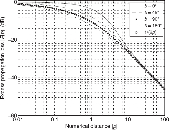
FIGURE 9.1 Excess groundwave propagation loss versus |![]() |.
|.

FIGURE 9.2 Phase of groundwave contribution versus |![]() |.
|.
Because the parameter ![]() is a scaled version of the distance R2, the actual distance at which fields transition from an inverse distance to an inverse distance squared dependence will depend on frequency and ground dielectric parameters. For example, consider a ground surface with dielectric constant 15 and conductivity 0.003 S/m. Assuming that these parameters are valid for frequencies from 100 kHz to 1 MHz, we can find for vertical polarization (using cos2 ψ2 ≈ 1) that |
is a scaled version of the distance R2, the actual distance at which fields transition from an inverse distance to an inverse distance squared dependence will depend on frequency and ground dielectric parameters. For example, consider a ground surface with dielectric constant 15 and conductivity 0.003 S/m. Assuming that these parameters are valid for frequencies from 100 kHz to 1 MHz, we can find for vertical polarization (using cos2 ψ2 ≈ 1) that |![]() | = 1 at a distance of approximately 515 km for the 100 kHz frequency but at approximately 5.4 km at 1 MHz. Thus, the 100 kHz ground wave will attenuate much more slowly than the 1 MHz ground wave. Propagation over terrain for which conductivity values are much larger (such as seawater) shows much slower rates of increase in
| = 1 at a distance of approximately 515 km for the 100 kHz frequency but at approximately 5.4 km at 1 MHz. Thus, the 100 kHz ground wave will attenuate much more slowly than the 1 MHz ground wave. Propagation over terrain for which conductivity values are much larger (such as seawater) shows much slower rates of increase in ![]() as the distance increases. In horizontal polarization, the corresponding distance at which |
as the distance increases. In horizontal polarization, the corresponding distance at which |![]() | = 1 for the example above is less than 2 m for both 100 kHz and 1 MHz. This result demonstrates that horizontally polarized groundwaves attenuate very rapidly and have little practical use. Our further groundwave studies will thus concentrate on vertical polarization: practical antennas for generating ground waves are generally vertically polarized.
| = 1 for the example above is less than 2 m for both 100 kHz and 1 MHz. This result demonstrates that horizontally polarized groundwaves attenuate very rapidly and have little practical use. Our further groundwave studies will thus concentrate on vertical polarization: practical antennas for generating ground waves are generally vertically polarized.
Our consideration here of fields that vary as one-over-distance-squared may raise questions about the absence of similar terms in the direct and reflected waves of equation (9.3). However, the “near-field” 1/R2 and 1/R3 terms of the direct and reflected waves will almost always be found negligible compared to the ground wave in the ![]() region, since distances for which |p| is large typically have much larger values of R1 and R2 (due to the
region, since distances for which |p| is large typically have much larger values of R1 and R2 (due to the ![]() factor in
factor in ![]() ). For smaller values of |p| but with R1 and R2 values sufficiently large (i.e., k R1
). For smaller values of |p| but with R1 and R2 values sufficiently large (i.e., k R1 ![]() 1, k R2
1, k R2 ![]() 1), again the “near-field” terms are negligible compared to the ground wave, so these terms can generally be neglected outside the near-field region of the antenna, even when the ground wave is included. See Ref. [7] for further discussion of this issue. We must also remember that the planar Earth theory applies only for distances up to approximately
1), again the “near-field” terms are negligible compared to the ground wave, so these terms can generally be neglected outside the near-field region of the antenna, even when the ground wave is included. See Ref. [7] for further discussion of this issue. We must also remember that the planar Earth theory applies only for distances up to approximately ![]() km, so the curves of Figure 9.1 become invalid for a |
km, so the curves of Figure 9.1 become invalid for a |![]() | value that depends on both the frequency and the complex permittivity of the ground
| value that depends on both the frequency and the complex permittivity of the ground ![]() .
.
9.2.1 Elevated Antennas: Planar Earth Theory
For transmitting and receiving antennas sufficiently close to the ground surface, the groundwave contribution dominates the received field, (1 − Γ) is approximately 2, and the field amplitude is ![]() . However, as transmitter and receiver heights are increased, direct and reflected wave contributions must be included, and the groundwave calculation is slightly modified. For vertical antennas “sufficiently close” to the ground, the physical heights of the antennas, h1 and h2, are replaced by “numerical antenna heights” q1 and q2
. However, as transmitter and receiver heights are increased, direct and reflected wave contributions must be included, and the groundwave calculation is slightly modified. For vertical antennas “sufficiently close” to the ground, the physical heights of the antennas, h1 and h2, are replaced by “numerical antenna heights” q1 and q2

where h1 and h2 represent the transmitter and receiver heights, respectively. Numerical antenna heights are defined similarly for horizontal antennas, but the above definition of q is multiplied by ![]() . Again, the numerical antenna heights depend on both frequency and
. Again, the numerical antenna heights depend on both frequency and ![]() and are scaled versions of the actual heights. Antenna elevation effects usually can be neglected for cases with q1 + q2 < 0.01.
and are scaled versions of the actual heights. Antenna elevation effects usually can be neglected for cases with q1 + q2 < 0.01.
For elevated antennas, spherical Earth theory shows that the planar Earth theory considered in equation (9.3) becomes invalid if either actual antenna height h1,2 becomes larger than approximately ![]() m. For antenna heights within these limits and for distances less than
m. For antenna heights within these limits and for distances less than ![]() km, the planar Earth theory remains valid, but calculation of groundwave contributions is slightly modified. Direct, reflected, and groundwave contributions are added in the proper phase relationships in equation (9.3), but the groundwave function F is calculated as
km, the planar Earth theory remains valid, but calculation of groundwave contributions is slightly modified. Direct, reflected, and groundwave contributions are added in the proper phase relationships in equation (9.3), but the groundwave function F is calculated as ![]() , where
, where ![]() Computation of this function versus distance can be quite tedious, so use of computers is recommended. An approximation for the total field is available for cases where p > 20, p > 10q1q2, and p > 100(q1 + q2). In this case, the resulting total field amplitude is simply that of the ground wave alone (assuming source and receiving antennas on the ground) multiplied by “height-gain” functions f(q1) and f(q2), where
Computation of this function versus distance can be quite tedious, so use of computers is recommended. An approximation for the total field is available for cases where p > 20, p > 10q1q2, and p > 100(q1 + q2). In this case, the resulting total field amplitude is simply that of the ground wave alone (assuming source and receiving antennas on the ground) multiplied by “height-gain” functions f(q1) and f(q2), where

This equation considerably simplifies calculations for elevated antennas that fall into the applicable region. A common procedure is to use (9.18) and to multiply the result by f(q1) f(q2). Figure 9.3 plots f(q) versus q for different values of b; note that increases in antenna height typically result in increases in received power, although there are some combinations of q and b for which reduced power is observed. This behavior occurs because increasing power in the direct and reflected waves as antenna heights increase is compensated by decreased power in the groundwave field, particularly for smaller values of b.

FIGURE 9.3 Planar Earth height-gain function f(q).
9.3 SPHERICAL EARTH GROUNDWAVE PREDICTION
When distances between the source and the receiver exceed ![]() km or when transmitting or receiving antenna heights are increased above
km or when transmitting or receiving antenna heights are increased above ![]() m, the effect of Earth curvature must be taken into account. The theory of groundwave propagation over a spherical Earth has been considered by many researchers, but the resulting expressions (which are obtained from a “Watson”-type transformation of a spherical eigenfunction solution) remain more complicated than those for the planar Earth model. The outcome of the theory is essentially that groundwave field amplitudes decay more rapidly than one-over-distance-squared at large distances. Refraction effects in the Earth atmosphere are approximately included through the use of the effective Earth radius aeff = κa described in Chapter 6.
m, the effect of Earth curvature must be taken into account. The theory of groundwave propagation over a spherical Earth has been considered by many researchers, but the resulting expressions (which are obtained from a “Watson”-type transformation of a spherical eigenfunction solution) remain more complicated than those for the planar Earth model. The outcome of the theory is essentially that groundwave field amplitudes decay more rapidly than one-over-distance-squared at large distances. Refraction effects in the Earth atmosphere are approximately included through the use of the effective Earth radius aeff = κa described in Chapter 6.
The distance d in the spherical Earth theory now refers to the distance measured along the arc length of the Earth. Groundwave predictions in this case are most conveniently evaluated in terms of a new scaled distance parameter x, defined as

The scaled distance x is related to the frequency and the effective Earth radius, but not to the dielectric properties of the ground. Note that for a fixed distance d, as frequency is increased, x will increase only as the cube root of the frequency. New scaled antenna heights y1,2 are defined through

and a new descriptor of the ground dielectric parameters τ is also defined:

Note that τ is related to the frequency in a fashion similar to x, except for variations in ![]() that occur with frequency.
that occur with frequency.
Field complex amplitudes for a vertically polarized source at distances beyond the planar Earth theory limit are expressed as

where the sum is over an index s to a set of complex “roots” ![]() , and where the
, and where the ![]() function is a spherical Earth height-gain function that also depends on s. Although the complexity of this expression makes obtaining insight difficult, values of
function is a spherical Earth height-gain function that also depends on s. Although the complexity of this expression makes obtaining insight difficult, values of ![]() are found to have negative imaginary parts so that each term in the series represents an exponential decay as the distance, and therefore x, increases. Also, because the imaginary parts of the roots
are found to have negative imaginary parts so that each term in the series represents an exponential decay as the distance, and therefore x, increases. Also, because the imaginary parts of the roots ![]() become more negative as s increases, the relative amplitudes of each term decrease with s so that the number of terms that must be included in the series for a given accuracy is reduced as the distance is increased. For distances
become more negative as s increases, the relative amplitudes of each term decrease with s so that the number of terms that must be included in the series for a given accuracy is reduced as the distance is increased. For distances ![]() km (so that x > 1.2 when a 4/3 Earth radius multiplier is used), neglecting all but the first series term typically results in errors no larger than approximately 10%. It should be noted that the above expressions are most effective for regions outside the planar Earth region and for antenna heights at which a direct line of sight is not obtained. For high antennas within the line of sight, a geometrical optics theory of reflection from a spherical Earth can be applied [8], but it is not considered here.
km (so that x > 1.2 when a 4/3 Earth radius multiplier is used), neglecting all but the first series term typically results in errors no larger than approximately 10%. It should be noted that the above expressions are most effective for regions outside the planar Earth region and for antenna heights at which a direct line of sight is not obtained. For high antennas within the line of sight, a geometrical optics theory of reflection from a spherical Earth can be applied [8], but it is not considered here.
The values of ![]() in equation (9.15) are obtained from another set of series expansions described in the appendix to this chapter. The spherical Earth height-gain functions
in equation (9.15) are obtained from another set of series expansions described in the appendix to this chapter. The spherical Earth height-gain functions ![]() and
and ![]() are also complicated and are again described in detail in the appendix. The approximate forms given in the appendix show that
are also complicated and are again described in detail in the appendix. The approximate forms given in the appendix show that ![]() is approximately linear in y for small antenna heights, but increases rapidly for larger heights. For consideration of cases where the groundwave mechanism is applicable (i.e., low frequencies), the elevated antenna procedures for the planar Earth model are usually reasonable, and the planar Earth height-gain functions can often be applied. Thus, approximating
is approximately linear in y for small antenna heights, but increases rapidly for larger heights. For consideration of cases where the groundwave mechanism is applicable (i.e., low frequencies), the elevated antenna procedures for the planar Earth model are usually reasonable, and the planar Earth height-gain functions can often be applied. Thus, approximating ![]() by f(q) when the conditions for using f(q) are satisfied will typically yield only minor errors.
by f(q) when the conditions for using f(q) are satisfied will typically yield only minor errors.
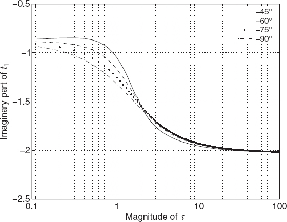
Figure 9.4 plots the excess propagation loss (determined from the field amplitude divided by 2E0/d) from the spherical Earth theory with both antennas on the ground and for three values of the ground parameter τ. Note that τ = 0 corresponds to perfectly conducting ground, while increasing values of τ for a fixed frequency indicate more poorly conducting grounds. The spherical Earth theory shows excess loss similar to that of the planar Earth theory (although the horizontal axes are scaled differently) for smaller distances, but exponential attenuation (which appears as a curved rather than linear dependency on a log–log scale) is evident at larger distances. The distance at which the exponential attenuation becomes predominant is again observed to depend significantly on the conductivity of the Earth. A plot of the spherical Earth height-gain function ![]() for the s = 1 term is illustrated in Figure 9.5 for three values of τ. The plot shows similar behaviors to the planar Earth height-gain function in that increases in antenna height can initially decrease field strength before dramatic increases are observed at larger heights. Height-gain functions show larger values for the poorer conducting grounds because field strengths at the surface are much smaller for this case.
for the s = 1 term is illustrated in Figure 9.5 for three values of τ. The plot shows similar behaviors to the planar Earth height-gain function in that increases in antenna height can initially decrease field strength before dramatic increases are observed at larger heights. Height-gain functions show larger values for the poorer conducting grounds because field strengths at the surface are much smaller for this case.

FIGURE 9.4 Spherical Earth excess propagation loss.

FIGURE 9.5 Spherical Earth height-gain function ![]() km.
km.
9.4 METHODS FOR APPROXIMATE CALCULATIONS
The complexity of the equations for groundwave computations can make predictions somewhat difficult. However, approximations can help with this process in many cases. For the planar Earth region with both antennas “on” the ground, the following steps can be useful:
- Compute the distance to which the planar Earth theory is valid:
 km.
km. - Evaluate the relationship between
 and distance d using equations (9.5) (vertical antennas) or (9.6) (horizontal antennas).
 - Values of the excess propagation loss in the planar Earth region can then be read approximately from Figure 9.1.
- For || > 20, the approximation
 yields acceptable accuracy. An inverse-distance squared dependence in field amplitudes will be obtained for all larger distances within the planar Earth theory limits.
 - If more accuracy is needed, an empirical approximation to
 is described in ref. [9] as
which is valid to within 3 dB with improved accuracy for b less than 35°.
- If even more accuracy is needed, the series forms of equations (9.8) and (9.9) can be computed and used.

For distances beyond the planar Earth theory limit with both antennas “on” the ground,
- Determine the relationship between the distance and the spherical Earth distance parameter x from equation (9.12).
- For distances
 km, retaining only a single term in the series (9.15) should yield acceptable accuracy.
 - When only a single term is needed, equation (9.15) can be simplified for field amplitudes to
FIGURE 9.6 Spherical Earth attenuation factor
 versus |τ|, with phase of τ as a parameter.
where Q is defined as a field scaling factor and is a function only of the ground dielectric descriptor τ.
- Figure 9.6 plots versus |τ|, while Figure 9.7 plots Q versus |τ|. The phase of τ is included as a parameter in the plots. Values read from these plots can be used in equation (9.17) to predict field strength for
 km. Exponential attenuation is obtained because the imaginary part of
  from Figure 9.6 is negative.
 - For distances between
 km and
  km, the above methods do not apply. However, because the transition in field behavior from the planar Earth to spherical Earth regions is typically very gradual, a simple smooth curve drawn to connect fields in the two regions will often yield reasonable accuracy.

9.5 A 1 MHz SAMPLE CALCULATION
Consider a 1 MHz vertically polarized transmitter transmitting 1 kW of power over “wet ground” with dielectric constant 30 and conductivity 0.01 S/m. For this case, the resulting complex dielectric constant is 30 − j179.8, and the planar Earth theory should apply for distances to approximately 80 km. If both transmitting and receiving antennas are located close to the ground, the received field is entirely due to the ground wave, and in the planar Earth region is

FIGURE 9.7 Spherical Earth field scaling factor Q versus |τ|, with phase of τ as a parameter.
where E0 for a short monopole antenna is 150 mV rms if d is measured in km in the above equation (i.e., the field strength produced by a short monopole antenna transmitting 1 kW of power above a perfectly conducting plane is 300 mV rms at distance 1 km).
Computation of the planar Earth “numerical distance” ![]() (using cos2 ψ2 ≈ 1) provides
(using cos2 ψ2 ≈ 1) provides

with d in km. Thus, at the distance at which the planar Earth theory becomes invalid, ![]() will obtain an amplitude of 4.6. The phase parameter b in this case is approximately 9.8°, indicating the relatively large conductivity of the ground. Due to the moderately small amplitudes of
will obtain an amplitude of 4.6. The phase parameter b in this case is approximately 9.8°, indicating the relatively large conductivity of the ground. Due to the moderately small amplitudes of ![]() that will be obtained for this problem in the planar Earth region, the series expansion of equation (9.8) can be used for all calculations. Figure 9.8 illustrates the resulting groundwave amplitude assuming that both antennas are located on the ground. Calculations are also included for distances greater than 80 km to investigate the inaccuracy of the planar Earth theory at larger distances. The transition from a one-over-distance to a one-over-distance-squared dependence is evident in the range from 10 to 100 km. Approximate predictions using equation (9.16) are valid for this case to within 0.4 dB at all the distances illustrated in Figure 9.8.
that will be obtained for this problem in the planar Earth region, the series expansion of equation (9.8) can be used for all calculations. Figure 9.8 illustrates the resulting groundwave amplitude assuming that both antennas are located on the ground. Calculations are also included for distances greater than 80 km to investigate the inaccuracy of the planar Earth theory at larger distances. The transition from a one-over-distance to a one-over-distance-squared dependence is evident in the range from 10 to 100 km. Approximate predictions using equation (9.16) are valid for this case to within 0.4 dB at all the distances illustrated in Figure 9.8.

FIGURE 9.8 Sample calculation at 1 MHz.
Spherical Earth theory results are also included in Figure 9.8 using equation (9.15) and the equations in the appendix assuming a 4/3 Earth radius multiplier. The spherical Earth distance x is related to the actual distance d through

with d in km. Note that the spherical Earth distance parameter x is 0.42 at distance 80 km, where spherical Earth results begin to be required. The spherical Earth dielectric parameter τ for this case is approximately 2.13 − j2.53 = 3.3e−j0.870, indicating again that the ground is a relatively good conductor. The results show a good match between the two theories even up to distances of about 100 km, but the spherical Earth exponential attenuation is clearly observed for larger distances. The approximate spherical Earth method described in equation (9.17) can be computed for this case by finding ![]() from Figure 9.6 and Q = −14.6 dB from Figure 9.7. Results from this approximation are within 0.5 dB of the complete series solution for distances greater than
from Figure 9.6 and Q = −14.6 dB from Figure 9.7. Results from this approximation are within 0.5 dB of the complete series solution for distances greater than ![]() . Behavior of the exact solution for distances between 80 and 241 km is indeed observed to be a smooth function of distance, so a simple curve drawn to connect the two regions would yield reasonable accuracy.
. Behavior of the exact solution for distances between 80 and 241 km is indeed observed to be a smooth function of distance, so a simple curve drawn to connect the two regions would yield reasonable accuracy.
At this relatively low-frequency, practical antenna elevations are likely to be very small compared to the 300 m wavelength, so elevated antenna effects are not likely to be observed.
9.6 A 10 MHz SAMPLE CALCULATION
Next, consider a 10 MHz vertically polarized transmitter transmitting 1 kW of power over ground with dielectric constant 15 and conductivity 0.003 S/m. For this case, the resulting complex dielectric constant is 15 − j5.4, and the planar Earth theory should apply for distances out to approximately 37 km.
Computation of the planar Earth “numerical distance” ![]() (using cos2 ψ2 ≈ 1) provides
(using cos2 ψ2 ≈ 1) provides

with d in km. Thus, at the distance at which the planar Earth theory becomes invalid, ![]() will obtain an amplitude of 229, much larger than in the 1 MHz example. The phase parameter b in this case is approximately 71.5°, indicating the relatively low conductivity of the ground. Due to the typically large amplitudes of
will obtain an amplitude of 229, much larger than in the 1 MHz example. The phase parameter b in this case is approximately 71.5°, indicating the relatively low conductivity of the ground. Due to the typically large amplitudes of ![]() that will be obtained for this problem in the planar Earth region, the series expansion of equation (9.9) can be used for almost all calculations. Figure 9.9 illustrates the resulting groundwave amplitude assuming that both antennas are located on the ground. Calculations are also included for distances greater than 37 km to investigate the inaccuracy of the planar Earth theory at larger distances. The relatively high frequency considered results in an inverse distance squared dependence for all the ranges illustrated in the figure. Approximate predictions using equation (9.16) are valid for this case to within 2.5 dB at all the distances illustrated in Figure 9.9; decreased accuracy is observed compared to the 1 MHz example due to the larger value of b.
that will be obtained for this problem in the planar Earth region, the series expansion of equation (9.9) can be used for almost all calculations. Figure 9.9 illustrates the resulting groundwave amplitude assuming that both antennas are located on the ground. Calculations are also included for distances greater than 37 km to investigate the inaccuracy of the planar Earth theory at larger distances. The relatively high frequency considered results in an inverse distance squared dependence for all the ranges illustrated in the figure. Approximate predictions using equation (9.16) are valid for this case to within 2.5 dB at all the distances illustrated in Figure 9.9; decreased accuracy is observed compared to the 1 MHz example due to the larger value of b.

FIGURE 9.9 Sample calculation at 10 MHz.
Spherical Earth theory results are also included in Figure 9.9 using equation (9.15) and the equations in the appendix assuming a 4/3 Earth radius multiplier. The spherical Earth distance x is related to the actual distance d through

with d in km. Again, the spherical Earth distance parameter x is 0.42 at distance 37 km where spherical Earth results begin to be required. The spherical Earth dielectric parameter τ for this case is approximately 3.75 − j23.0 = 23.3e−j1.41, indicating again that the ground is a relatively poor conductor. The results show a good match between the two theories even up to distances of about 40 km, but the spherical Earth exponential attenuation is clearly observed for larger distances. The approximate spherical Earth method described in equation (9.17) can be computed for this case by finding ![]() from Figure 9.6 and Q = −49.8 dB from Figure 9.7. Results from this approximation are within 0.5 dB of the complete series solution for distances greater than
from Figure 9.6 and Q = −49.8 dB from Figure 9.7. Results from this approximation are within 0.5 dB of the complete series solution for distances greater than ![]() . Again, behavior of the exact solution for distances between 40 and 112 km is observed to be a smooth function of distance.
. Again, behavior of the exact solution for distances between 40 and 112 km is observed to be a smooth function of distance.
For this higher frequency, reasonable antenna elevations can have a more significant effect. Consider elevated transmitting and receiving antennas with the transmitter at height 80 m and the receiver at height 10 m. In the planar Earth theory, the numerical antenna heights q1 and q2 at distances greater than 0.5 km are 4.07 and 0.509, respectively, so a significant influence of the elevated antenna heights should be expected. The simplified planar Earth height-gain function of equation (9.11) is applicable only for distances at which p > 20, p > 10q1q2, and p > 100(q1 + q2); the final condition implies distances greater than the planar Earth theory boundary of 80 km. Thus, planar Earth elevated antenna effects must be calculated from equation (9.3) including direct, reflected, and groundwave contributions (using ![]() as described in Section 9.2.1) appropriately. This is most easily accomplished through use of a computer. Spherical Earth results are also modified through use of the spherical Earth height-gain functions described in the appendix. Figure 9.10 plots the modification of field amplitudes obtained with these antenna heights, including planar Earth (solid) and spherical Earth (dashed) results. The larger antenna heights considered here result in an increase in received power of approximately 12.5 dB. A test of the approximate planar Earth height-gain functions for distances greater than 80 km also yields a value of 12.5 dB.
as described in Section 9.2.1) appropriately. This is most easily accomplished through use of a computer. Spherical Earth results are also modified through use of the spherical Earth height-gain functions described in the appendix. Figure 9.10 plots the modification of field amplitudes obtained with these antenna heights, including planar Earth (solid) and spherical Earth (dashed) results. The larger antenna heights considered here result in an increase in received power of approximately 12.5 dB. A test of the approximate planar Earth height-gain functions for distances greater than 80 km also yields a value of 12.5 dB.
9.7 ITU INFORMATION AND OTHER RESOURCES
ITU-R Recommendation P. 368-9 [10] provides several curves for the prediction of groundwave intensity produced by a 1 kW short vertical monopole antenna at ground level. Curves are presented for varying ground dielectric constants, conductivities, and frequencies, enabling a time-consuming computation to be avoided for many cases. However, the curves apply only for both transmitting and receiving antennas near the ground; for elevated antennas, the height-gain functions must still be applied. These curves were produced using an exponential model for the atmospheric refractive index, which should be more accurate than the linear refractive index model implicit in the modified Earth radius assumption, because the exponential model avoids the exaggerated decrease in atmospheric refractivity with altitude of the linear model. Five sets of curves resulting from the ITU model are presented in Figures 9.11–9.15. It should be noted that the results presented in this section and the models described in this chapter apply for groundwave propagation predictions on average; for a given measurement, site-specific terrain effects may cause significant deviations from these predictions.
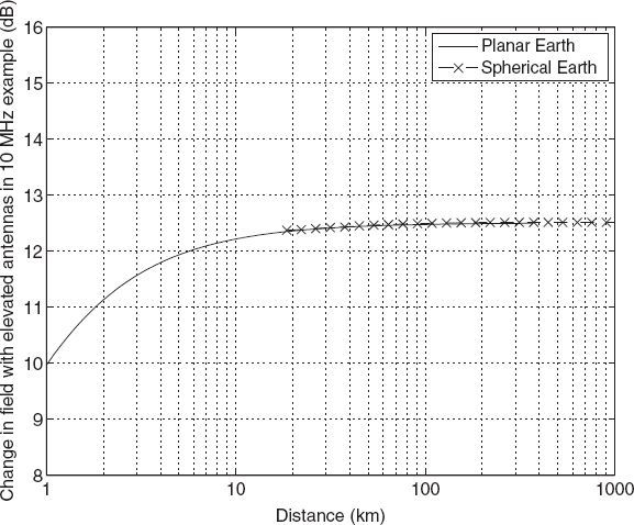
FIGURE 9.10 Change in received power with elevated antennas for sample calculation at 10 MHz.
Methods for predicting groundwave propagation over mixed paths, that is, paths that are part ground and part sea, for example, or over layered ground surfaces (such as ice-covered seawater) have also been developed; these issues are described in Ref. [7]. In Ref. [11] an empirical model for groundwave propagation in urban areas is described.
9.8 SUMMARY
The groundwave propagation mechanism is important when both transmitting and receiving antennas are relatively close to the ground in terms of the electromagnetic wavelength. The resulting field transitions from 1/d to 1/d2 to exponential decay with distance at a rate that depends on the frequency and ground dielectric parameters. Use of the “numerical” distance clarifies the relative influence of these physical parameters. Groundwave contributions are usually not significant at VHF and higher frequencies. At lower frequencies, the distance to which they are important varies, generally increasing with decreasing frequency, and also depending on the ground constants and other system parameters. If ionospheric propagation is strong, ionospheric signals often dominate the groundwave mechanism.

FIGURE 9.11 Groundwave curves for “seawater, low salinity” with relative dielectric constant 80, conductivity 1 S/m. (Source: ITU-R Recommendation P. 368-9, used with permission.)

FIGURE 9.12 Groundwave curves for “freshwater” with relative dielectric constant 80, conductivity 0.003 S/m. (Source: ITU-R Recommendation P. 368-9, used with permission.)

FIGURE 9.13 Groundwave curves for “wet ground” with relative dielectric constant 30, conductivity 0.01 S/m (Source: ITU-R Recommendation P. 368-9, used with permission.)
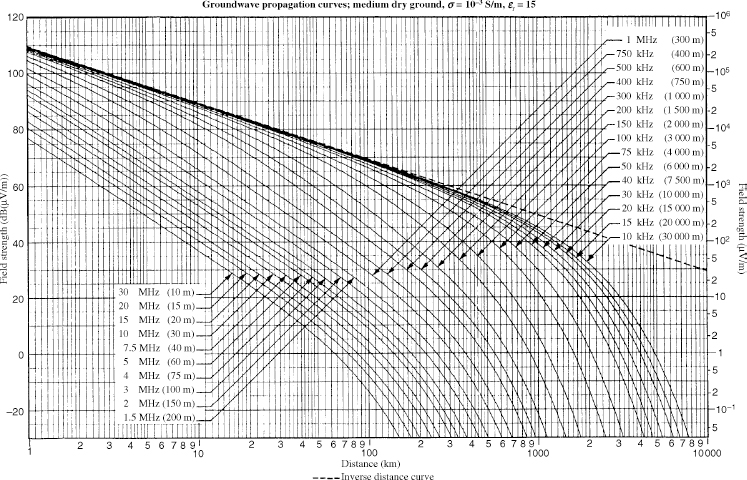
FIGURE 9.14 Groundwave curves for “medium dry ground” with relative dielectric constant 15, conductivity 0.001 S/m. (Source: ITU-R Recommendation P. 368-9, used with permission.)
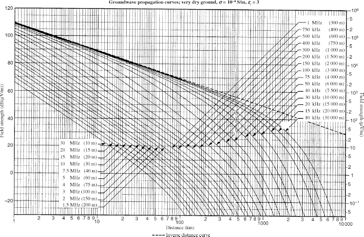
FIGURE 9.15 Groundwave curves for “very dry ground” with relative dielectric constant 3, conductivity 0.0001 S/m. (Source: ITU-R Recommendation P. 368-9, used with permission.)
APPENDIX 9.A SPHERICAL EARTH GROUNDWAVE COMPUTATIONS
The “roots” ![]() appearing in the spherical Earth theory can be obtained from a series expansion [12]:
appearing in the spherical Earth theory can be obtained from a series expansion [12]:

where τ is the spherical Earth dielectric parameter, ![]() exp (−jπ/3) (values of ts,0 for s = 1, 2, ··· 5 are given in Table 9.1),
exp (−jπ/3) (values of ts,0 for s = 1, 2, ··· 5 are given in Table 9.1), ![]() , and for n > 0,
, and for n > 0,
with ![]() for all n ≠ 2, but
for all n ≠ 2, but ![]() for n = 2. For s > 5, ts,0 can be obtained from
for n = 2. For s > 5, ts,0 can be obtained from
The series in equation (9.23) converges well for small amplitudes of τ; for larger amplitudes, a different series is more useful:
TABLE 9.1 Values of ts,0 and ts,∞ for s from 1 to 5

where ![]() exp (−jπ/3) (values of ts,∞ for s = 1, 2, · · · 5 are given in Table 9.1), and
exp (−jπ/3) (values of ts,∞ for s = 1, 2, · · · 5 are given in Table 9.1), and


For s > 5, ts,∞ can be approximated as
The series expansion (9.26) is typically useful when ![]() and that of equation (9.23) otherwise.
and that of equation (9.23) otherwise.
The height-gain functions for the spherical Earth theory ![]() are defined as
are defined as
where ![]() is the sth spherical Earth “root” defined above, and
is the sth spherical Earth “root” defined above, and
Ai and Bi above are the Airy functions of the first and second kinds, respectively. For small values of y, the spherical Earth height-gain functions can be approximated by

while for values of y such that ![]() ,
,

Given the large number of calculations required for groundwave predictions, computer programs have been developed to avoid much of the tedium and are recommended for general use. An example is the GRWAVE package available from the ITU.
REFERENCES
1. Sommerfeld, A. N., “Propagation of waves in wireless telegraphy,” Ann. Phys., vol. 28, pp. 665–737, 1909.
2. Sommerfeld, A. N., “Propagation of waves in wireless telegraphy II,” Ann. Phys., vol. 81, pp. 1135–1153, 1926.
3. Van der Pol, B., and H. Bremmer, “The diffraction of EM waves from an electrical point source round a finitely conducting sphere with applications to radiotelegraphy and the theory of the rainbow I,” Phil. Mag. vol. 24. pp. 141–176, 1937.
4. Van der Pol, B., and H. Bremmer, “The diffraction of EM waves from an electrical point source round a finitely conducting sphere with applications to radiotelegraphy and the theory of the rainbow II,” Phil. Mag. vol. 24, no. 164, pp. 825–864, 1937.
5. Van der Pol, B., and H. Bremmer, “The propagation of radio waves over a finitely conducting spherical Earth,” Phil. Mag. vol. 25, pp. 817–834, 1938.
6. Norton, K. A., “The calculation of groundwave field intensity over a finitely conducting spherical Earth,” Proc. IRE, vol. 29, p. 623, 1941.
7. Wait, J., “The ancient and modern history of electromagnetic groundwave propagation,” IEEE Antennas Propag. Mag., pp. 7–24, 1998.
8. Fishback, William T. “Methods for calculating field strength with standard refraction,” in Kerr, Donald E. (ed.), Propagation of Short Radio Waves, McGraw-Hill, New York, 1951, pp. 112–140.
9. Li, R., “The accuracy of Norton's empirical approximations for groundwave attenuation,” IEEE Trans. Antennas Propag., vol. 31, pp. 624–628, 1983.
10. ITU-R Recommendation, P. 368–9, “Ground-wave propagation curves for frequencies between 10 kHz and 30 MHz,” International Telecommunication Union, 2007.
11. Lichun, L., “A new MF and HF ground wave model for urban areas,” IEEE Antennas Propag. Mag., pp. 21–33, 2000.
12. Logan, N. A., and K. S. Yee, “A mathematical model for diffraction by convex surfaces,” in Electromagnetic Waves, (R. E. Langer, ed.), University of Wisconsin Press, Madison, WI, 1962.
Radiowave Propagation: Physics and Applications. By Curt A. Levis, Joel T. Johnson, and Fernando L. Teixeira
Copyright © 2010 John Wiley & Sons, Inc.
1Section 9.2 is based on the work of K. A. Norton [6].