10

CHARACTERISTICS OF THE IONOSPHERE

10.1 INTRODUCTION¹

The region of the Earth's atmosphere from approximately 40 km altitude out to several Earth radii is known as the ionosphere. In this region, solar and cosmic radiation ionize neutral particles to produce regions of space containing large numbers of positively charged ions and free electrons, with peak electron densities of about N_e = 10⁶ particles/cm³ at an altitude of about 300 km. The presence of free electrons has a significant effect on wave propagation at HF and lower frequencies, allowing for propagation over long distances through ionospheric reflections, as we will discuss in Chapter 11.

The physics of the ionosphere, essentially involving the chemistry of the upper atmosphere and its interaction with solar radiation, has been studied extensively [1], but can be very complex. Factors that can influence the ionosphere include the Earth's magnetic field, the amount of ionizing radiation obtained from the Sun (which can increase dramatically in periods of high “solar activity”), and atmospheric chemistry and mixing. In this chapter, we will study one of the basic theories that describes the electron/ion production and recombination rates in an ionospheric “layer” [2,3]. This theory, developed by Chapman, will turn out to be applicable mainly to the so-called E and F₁ regions of the ionosphere, but provides useful insight into the behavior of other regions as well. We will also consider the basic structure of the ionosphere and briefly examine the influence that the Sun and its solar cycle have on ionospheric ionization. Note that the terms “layer” and “region” for describing portions of the ionosphere are used interchangeably in the literature because the ionosphere was thought to consist of distinct layers in the early days of radio; in fact, the electron density is a continuous function of altitude. Nevertheless, certain regions are found to reflect or absorb radio waves in a relatively uniform way, distinct from other regions. While it is more accurate to refer to them as regions, the earlier nomenclature has persisted, and the terms “region” and “layer” are also used here without distinction.

10.2 THE BAROMETRIC LAW

We shall consider the production of ionized layers by solar radiation, mostly X-ray and ultraviolet. This radiation interacts with neutral molecules of the atmosphere to produce electron/ion pairs. It is therefore of interest to examine first the distribution of the molecules as a function of height.

Consider a small cylindrical volume of arbitrary cross section A and length dh, as shown in Figure 10.1. Let its axis be vertical. Denote the pressure at the bottom by p, corresponding to the height h. At the top, the height is h + dh and the corresponding pressure is p + dp. Since atmospheric pressure decreases with height, dp will be a negative quantity when dh is positive.

The external atmosphere exerts a vertical, buoyant force on this volume by virtue of the pressure difference between the top and bottom surfaces. A force of magnitude Ap pushes up on the bottom, a force A(p + dp) pushes down on the top, and the net upward differential force on the volume is therefore the buoyant force

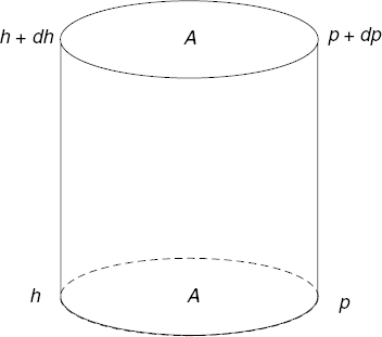
FIGURE 10.1 Differential atmospheric volume.

Assuming equilibrium to exist (i.e., no vertical wind), this force must be precisely balanced by the downward gravitational force. The differential weight of the gas in the volume is

where ρ is the mass density of the gas (mass per unit volume) and g is the gravitational constant. The density is given by

where N is the number density (number of molecules per unit volume) and m_s is the mean molecular mass. Thus, the differential gravitational force is

Equating this to the buoyant force gives

From the ideal gas law of physics, p = Nk_BT, where k_B is Boltzmann's constant and T is the absolute temperature, so

and use of this in equation (10.5) gives

which may be integrated to yield

or

The left-hand side is ln [p(h)/p(h₀)], so that we can write

In the above integral, k_B is a true constant and g is very nearly constant since the scale of height variations considered is small compared to the distance from the Earth's center. On the other hand, m_s depends on h since heavier molecules are most abundant at low altitudes. Furthermore, the temperature T can be a quite complicated function of altitude. However, over limited distances the whole integrand may often be considered nearly constant. In that case, denoting

we get

Finally, by again using the ideal gas law and assuming an isothermal condition, we obtain

and, by the use of equation (10.3),

The dimensions of H are the same as those of h, that is, length. The pressure, mass density, and number density are seen to vary exponentially with height difference measured in H-units. H is therefore called “the local scale height”: it scales the height difference and is local in the sense that the concept breaks down over height differences over which the mean molecular mass or the temperature varies significantly.

The reference height h₀ in this development is arbitrary. For some purposes, it may be assumed to be sea level. In the Chapman theory of the formation of ionized regions, it will turn out handy to choose the height of maximum ion production as the reference height. Figure 10.2a illustrates a typical plot of ρ and p versus altitude; note that a log scale is used so that the barometric curve should appear as a straight line with a slope determined by the scale height. The fact that scale height changes with altitude in the atmosphere is indicated by the curved nature of these plots versus height. Figure 10.2b displays the scale heights H associated with the pressure and density as a function of altitude. Figure 10.3 provides plots versus altitude of several atmospheric quantities. Information such as this is available from the U.S. National Oceanic and Atmospheric Administration (NOAA) [4].

FIGURE 10.2 Typical plot of atmospheric density versus altitude. (Source: U.S. Standard Atmosphere, NOAA/NASA [4].)

FIGURE 10.3 Sample atmospheric data. (Source: U.S. Standard Atmosphere, NOAA/NASA [4].)

These figures show the expected dependencies of decreasing pressure, density, and collision frequencies in the atmosphere as altitude increases. The decrease in mean molecular weight observed is due the change in chemical composition of the atmosphere for increasing altitudes, caused by decreasing fractions of molecular oxygen O₂ and nitrogen N₂. Atmospheric temperature also varies significantly with altitude; note the temperature is a measure of the average kinetic energy of molecules in the atmosphere, even for the very low atmospheric densities encountered at high altitudes. One broad division of the atmosphere into two regions is based on the amount of mixing of species. For altitudes below circa 90 km, turbulent mixing causes a more uniform atmospheric composition, and this region is labeled the homosphere. At higher altitudes, the atmosphere is less well mixed, and this region is thus labeled the heterosphere.

10.3 CHAPMAN'S THEORY

10.3.1 Introduction

Chapman was the first to formulate a quantitative theory of the formation of ionized regions in the atmosphere due to ionizing radiation from the Sun [2]. A qualitative picture of the process is relatively easy to obtain. At very high altitudes, there is plenty of solar flux but there are few molecules available to be ionized. Hence, ion production will be small at very high altitudes. At low altitudes, there are plenty of molecules to be ionized, but most of the flux has been used up at higher levels; again, ion production will be small. At some intermediate altitude, there will be sufficient molecules and sufficient flux to maximize ion production. Hence, the production of electron–ion pairs increases monotonically from low values at low altitudes to a maximum at some intermediate altitude and then decreases monotonically at higher altitudes.

The mathematical development of this relationship will proceed along the following steps:

(a) The amount of solar flux penetrating to a height h will be calculated. An important parameter will be the “optical depth”, a measure of the opacity of the region above height h.

(b) By differentiation of the flux expression, the decrease in flux in an incremental height dh will be found.

(c) The flux decrease represents absorbed power, which is responsible for the ionization. From this principle, an expression for the ion production per unit volume at height h will be derived.

(d) The barometric law will be used to find the optical depth explicitly as a function of height. In order to simplify the equations, the reference height will be chosen as the height where the optical depth is unity.

(e) The height of maximum possible electron/ion production will be shown to be the reference height.

(f) From the law of electron/ion production and the assumption of equilibrium, laws of the variation of electron density will be derived.

(g) The electron/ion production and electron density depend on two variables: altitude and solar zenith angle. By developing suitable scaling laws, it will be found they can be represented as functions of a single variable.

10.3.2 Mathematical Derivation

(a) We first calculate the amount of solar flux S as a function of the height h. Consider a cylinder of arbitrary cross section A with its axis inclined with respect to the vertical by the solar zenith angle χ, as shown in Figure 10.4.

The flux density at the top (height h + dh) is S + dS, and that at the bottom is S. The loss of flux in the volume is therefore A dS. This flux is absorbed by the molecules in the cylinder. Let the average absorption cross section (i.e., the power absorbed per molecule per unit flux, averaged over the various molecular species) be denoted by σ (units of area). Then

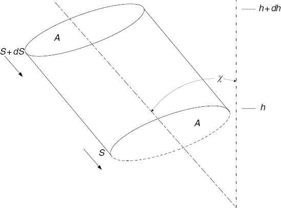
FIGURE 10.4 Tilted differential atmospheric volume.

where N is again the number density of molecules and dV is the differential volume given by

Use of this in equation (10.15) and division by AS gives

which can be integrated to give

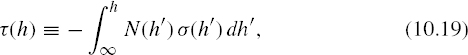
Define the optical depth τ(h) (a unitless quantity) by

then

and therefore

where S_∞ = S(∞) denotes the flux at a very large height, so that all absorption above it is negligible.

(b) The change in flux density per unit height increment can now be obtained by differentiation:

The value of dτ/dh follows from the definition of τ as an integral in equation (10.19):

and thus we get

(c) The power absorbed in the volume is given by

If we denote the number of ions produced in the volume per unit time as n_i, then

where ς denotes the ionization efficiency, that is, the number of ions produced per unit time per unit power. Thus,

is the number of ions produced per unit time in the volume by the conversion of radiant flux energy to ionization energy.

Let q denote the rate of ion production per unit volume. Then

By equating (10.27) and (10.28), we get

and using equation (10.24) gives

So far the treatment has been quite general. Although some new notations were used, no restrictive assumptions were made. At this point, if an analytical (as opposed to numerical) approach is to be carried further, some simplifying assumptions are necessary.

(d) Assume that over the region of interest the absorption cross section σ and ionization efficiency ς do not vary appreciably. These quantities depend on the mixture of molecular species. Also, assume that N(h) follows the barometric law of equation (10.13). Then from the definition of τ in equation (10.19), we get

By putting h = h₀ in this equation, we find

so equation (10.31) can also be written as

To eliminate the constants σN(h₀)H = τ(h₀) from the remainder of this development, we now choose the reference height h₀, which is arbitrary, so that τ(h₀) = 1. This choice also has physical significance. From equation (10.21), it can be seen that the reference height will then be the height for which, when the Sun is at zenith (χ = 0), the flux S(h₀) will have decreased to 1/e (or 37%) of its incident value S_∞. It will also be shown later that, for the Sun at zenith, the electron–ion production rate q(χ = 0, h) is maximum at h = h₀. Using the further simplifying notation

gives

and from equation (10.32) with τ(h₀) = 1,

Use of these in equation (10.30) gives

(e) We are now ready to prove the previous statement that q is maximized at χ = 0, h = h₀. From the definition of z, equation (10.34), the condition h = h₀ is the same as z = 0. One small notational issue should be mentioned here. When the production rate q(χ, h) is expressed as a function of z, the form of the functional dependence changes since not h but (h − h₀)/H is replaced by the new variable z. So we should write to emphasize that they refer to two distinct mathematical expressions. However, since and q(χ, h) denote the same physical quantity, it is more convenient to adopt the “physicist practice” of using the same symbol for both and, if necessary, distinguishing them by their arguments

To maximize q(χ, z), we note by inspection that sec χ = 1 maximizes the expression with respect to χ for all z, giving

To maximize this with respect to z, find

Requiring leads to e^−z − 1 = 0, and therefore z = 0 or h = h₀. The value of q(χ, z), maximized with respect to both solar zenith angle and height, is then

Hence,

and by the use of this in (10.39), we get

(f) For ionospheric path calculations, we are not interested so much in the electron/ion production rate q(χ, z) as in the resulting electron density N_e, which will strongly affect electromagnetic wave propagation as discussed in Chapter 11. The function N_e(χ, h) can be derived by writing an equation for the net rate of change in electron density per unit volume as the difference between the rate of production q and the rate of electron loss r

In the actual ionosphere, many electrons are produced and lost in the time required to produce an appreciable change in the resulting electron density: on the timescale appropriate to the terms on the right-hand side of (10.45), the ionosphere is in equilibrium. We can therefore set the left-hand side equal to zero and obtain

There are numerous reactions that can remove free electrons from the ionosphere, and indeed it is difficult to go very far into the properties of the ionosphere without considering its chemistry, but that is beyond the scope of this book. Two classes of electron–loss processes can be distinguished: in the first, known as recombination, the electron combines with a positive ion to form a neutral molecule; in the second, known as attachment, it attaches itself to a neutral molecule to form a negative ion.

The recombination process depends on electrons finding ions: for this kind of process,

where α is a recombination coefficient, N_e is the electron density, and N_i is the ion density. Since ionization produces electrons and positive ions in equal numbers, N_i = N_e and

From (10.46), we then have

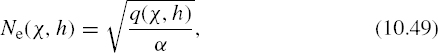
and using equation (10.44) and setting

gives

For the electron–molecule attachment process, the electrons have to find neutral molecules, and the number of these is independent of the number of electrons. Then the electron loss rate is

where is used to distinguish the attachment process electron density from N_e for the recombination process, is an attachment coefficient, and

From the barometric equation, (10.13) or (10.36), it follows that

or

Setting the electron production and loss rates equal as demanded by (10.46), we have

and use of equation (10.44) gives

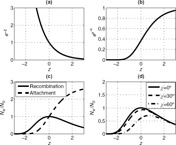
FIGURE 10.5 An illustration of functions involved in the Chapman theory: (a) a plot of e^−z, (b) a plot of exp (e^−z), (c) N_e/N₀ for recombination and attachment layers, and (d) impact of the solar zenith angle χ on a recombination layer.

Equations (10.51) and (10.57) have achieved the goal of this rather lengthy derivation because it is the electron density that relates most strongly to radiowave propagation effects, as will be discussed in detail in the next chapter. The mass of an electron is such that it can respond to radio waves with substantial motion, especially at HF and lower frequencies. The mass of ions is much greater. Therefore, ionic motions are much smaller, and the influence of ions can be neglected in usual propagation problems.

The nature of the layers predicted by equations (10.51) and (10.57) is somewhat difficult to discern directly, due to the double exponential functions involved. Figure 10.5 provides an illustration to clarify the layer shapes for χ = 0. Figure 10.5a is a plot of the function e^−z, one of the factors that determines the shape of the recombination layer of equation (10.51). This term is multiplied by the function exp (e^−z), plotted in Figure 10.5b, which ranges from 0 to unity as altitude increases. The product of these two clearly will produce a function that is maximum somewhere at middle altitudes; Figure 10.5c compares the electron density profile (divided by N₀) for recombination and attachment layers. The latter (equation (10.57)) is smaller for lower altitudes due to the increased atmospheric density and reattachment rate at lower altitudes. Figure 10.5d illustrates the influence of the solar zenith angle on a recombination layer; as the solar angle increases, the peak electron density decreases, and the height of the maximum increases in altitude.

(g) The electron production rate q(χ, z) and the resulting electron density distributions N_e(χ, z) and are functions of the two independent variables χ and z. It turns out, however, that values for arbitrary χ can be obtained rather simply from the values for χ = 0 by use of scaling laws. The scaling law for q(χ, z) will now be developed.

Suppose we are interested in q for a particular set of values χ₁, z₁. Instead of calculating it directly from equation (10.44), let us calculate a related value: that of q(0, z₁ − ln sec χ₁), that is, the production rate that corresponds to a zenith angle of zero and a normalized height z that corresponds to the desired value z₁ reduced by the log secant of the desired zenith angle. By equation (10.44), we have

Since e^{ln u} = u, we can transform this into

Now evaluate q(χ₁, z₁) by (10.44); the result is

Comparison of the last two relationships gives

Multiplying by cos χ₁, and then recalling that (z₁, χ₁) are arbitrary values of (z, χ), we can write

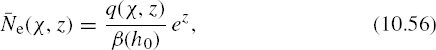
This is the desired scaling law. It says that a curve of q versus z for a zenith angle χ = 0 is really all we need. The value of q for any value of z and χ can be obtained from the χ = 0 curve at a z value equal to the true z reduced by ln sec χ, multiplied by cos χ. Similar scaling laws can be obtained for electron densities under the previous assumptions of recombination (N_e) and attachment . They are, respectively,

and

10.4 STRUCTURE OF THE IONOSPHERE

The upper part of Figure 10.6 depicts the nomenclature used in describing the atmosphere, including the ionosphere. The electron density sketch is not meant to represent typical conditions but has been drawn to allow representation of all possible “layers”. A more typical plot of electron density versus height is shown in the lower part of Figure 10.6, generated from the International Reference Ionosphere (IRI) for the location of Columbus, OH, on 07/01/2007 (12:00 PM).

FIGURE 10.6 The upper plot depicts standard atmospheric nomenclature versus altitude. (Source: T. E. Van Zandt, “The Formation of the Ionosphere,” Lecture 4 in NBS Course in Radio Propagation: Ionospheric Propagation, Central Radio Propagation Laboratory, National Bureau of Standards, U.S. Department of Commerce, Boulder, CO, 1961.) The lower plots are an example of the electron density distribution versus height generated by the International Reference Ionosphere for Columbus, OH, on 07/01/2007 (local noon). Left shows a larger range of altitudes while right shows more clearly the E region maximum near 110 km, the F₁ region from about 120 to 180 km, and the F₂ region above 180 km. The electron number densities (N_e) shown in these plots are in units of cm⁻³.

TABLE 10.1 Typical Ionospheric Regions (or Layers)

Note the two distinct curves for day- and nighttime electron densities: solar ionization during the day produces larger electron densities that gradually recombine at night through processes that vary with altitude. The particular molecular species that become ionized are indicated on the plot as well, with O₂ and N₂ molecules more prevalent at lower altitudes, and oxygen atoms at higher altitudes. Standard terminology usually defines three layers in the ionosphere, denoted by the letters D, E, and F with increasing altitude. The typical altitudes for these regions are indicated in the figure. The F and (rarely) E regions can also be subdivided into F₁ and F₂, and (rarely) E₁ and E₂ layers, with the lower subscript numbers referring to lower altitudes. Note the disappearance of the D layer at night. Table 10.1 summarizes information on ionospheric regions and layers. We will find in Chapter 11 that the D region primarily causes absorption and not reflection for MF and higher frequencies, so its absence at night allows MF frequencies to reach the E layer and be reflected. The F₁ and F₂ regions also combine into a single F region at night, and all layers have a reduced electron density since solar flux is no longer available to maintain the ionization process. Peak electron densities of about N_e = 10⁶ particles/cm³ occur in the F₂ layer. The N_e profile can have a secondary local maximum at about 100 km in the E region. In the D layer below 60 km, N_e drops precipitously to densities below N_e = 10³ particles/cm³.

In practice, it is found that the E and F₁ regions behave in a manner predicted rather well by equation (10.51). That equation, which specifies a recombination-type Chapman layer, is therefore of great importance. This is not true of equation (10.57), which gives the electron density of attachment-type Chapman layers: no extended ionospheric regions follow this law. Attachment may nevertheless be an important component of the ionospheric chemistry, especially in the D region. Ionization at higher altitudes than the F₁ layer is strongly influenced by the Earth's magnetic field and by mixing in the upper atmosphere, and is very complex. It is the F₂ region, however, that is of the greatest importance for HF communications, as we shall see in Chapter 11.

In addition to the day and night variations, ionospheric properties also vary with latitude, season, and solar cycles. Due to difficulties in the theoretical modeling of ionospheric properties, empirical methods are very important in predicting ionospheric propagation. A global network of ground-based ionospheric observation stations, which produce ionograms as described in Chapter 11, exists to allow for forecasting the expected behaviors (bottom-side sounders). Figure 10.7 illustrates the locations of many such ground stations.

This ground-based network can be augmented by a variety of space-based data from satellites (topside sounders). As the name indicates, bottom-side sounders refer to those suited for gathering ionospheric data below the F₂ peak, while topside sounders are suited for gathering data above it. Ionospheric properties can be further monitored using dual-frequency signals received from networks of GPS (or other global navigation satellite systems) receivers or from low-Earth orbit satellites using radio occultation techniques, as discussed in Chapter 11.

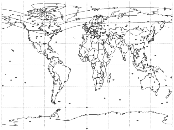
FIGURE 10.7 Sample locations of ionospheric observation stations. (Source: UK Solar System Data Centre, Science and Technology Facilities Council.)

One important source of ionospheric data is the International Reference Ionosphere (IRI) [5,6], an international project sponsored by the Committee on Space Research (COSPAR) and the International Union of Radio Science (URSI). This is a continuously updated empirical model of the ionosphere, based on a worldwide network of Earth-based and satellite-based ionospheric observation facilities. For a given geographical location, this model provides monthly averages of ionospheric parameters in the 50–2000 km height region. IRI information is currently distributed by NASA Goddard Space Flight Center and is freely available online.

Another useful ionospheric model is the NeQuick ionospheric electron density model [7], developed by the Abdus Salam International Centre for Theoretical Physics in Italy and by the University of Graz in Austria. Both models have been adopted by ITU-R Recommendation P.531, which deals with trans-ionospheric propagation [8].

10.5 VARIABILITY OF THE IONOSPHERE

From the Chapman theory, it is clear that geographic location, day of the year, and local time of day strongly affect the ionization of the E and F₁ regions through the Sun's zenith angle. It turns out that these parameters also strongly affect the F₂ region, although it is not a Chapman layer. The ionosphere is also subject to less predictable variations. These are due, in part, to atmospheric motions, and in part to variations in the emissions from the Sun. The atmosphere at ionospheric heights is not stationary. It exhibits currents and tides, somewhat analogous to those in the ocean though of course not stemming from the same causes. Though exhibiting a consistent pattern, these motions also vary. A propagation phenomenon that appears to be related to these motions is called “spread-F” [9]. When spread-F is active, F region reflections come from a great many altitudes instead of a single layer, and these altitudes depend rather randomly on the frequency of the signal. This makes broadband communications difficult.

Another propagation effect that appears to be at least partially related to atmospheric circulation is “sporadic E”, denoted by E_s. This manifests itself as a thin layer at the altitude of the normal E region, that is, near 100 km height, with an enhanced electron density comparable to that in the F region. As a result, signals intended for long-range communication via the F layer are reflected before they reach that layer, thus interfering with long-range communications. On the other hand, communication using E_s is enabled at shorter ranges, but cannot be depended upon because E_s occurs only sporadically. Radio amateurs sometimes exploit this method of communication.

Since solar flux is the cause of ionization in the ionosphere, variations in solar flux can have strong effects on atmospheric ionization and ionospheric propagation. Only a very brief introduction to these effects can be given here. The reader is referred to the literature [10] for a more detailed discussion. Ionization is primarily produced by the ultraviolet and X-ray portions of the solar flux, but particles ejected from the Sun also cause ionization, especially during periods of high solar activity. Although the amount of visible radiation from the Sun changes little from day to day, ultraviolet and X-ray radiation may change appreciably, resulting in variability in ionospheric propagation. Periods of high solar activity have been found to correlate well with the appearance of “sunspots” on the Sun's surface. These are dark regions that are of lower temperature than the surrounding surface. The average number of sunspots has been found to follow an 11-year cycle. Figure 10.8 illustrates the averaged sunspot number observed from 1940 to 2008 and also shows how this number correlates with the total averaged observed solar radiowave flux measured at f = 2.8 GHz (corresponding to λ = 10.7 cm), a widely used index of solar activity. Note that daily sunspot numbers can vary significantly from the averaged values. Sometimes no sunspots or flares are visible over a period of several weeks or months. Typically, the average annual 10.7 cm solar flux varies between about 70 s.f.u. (when no sunspots are present) and 250 s.f.u. The sunspot number is commonly used in empirical formulas for ionospheric propagation.

Solar events such as flares and coronal mass ejections are also correlated with the sunspot number. Figure 10.9 is an image of the Sun's surface with such features. In these events, large numbers of particles are emitted from the Sun's surface and spread throughout space to reach the planets. During such solar bursts, the measured solar flux density can reach much higher values.

The Earth's magnetic field, with a magnitude between about 3 × 10⁻⁵ and 5 × 10⁻⁵ T, is essentially that of a dipole. The Earth's magnetic field interacts with these charged particles from the Sun (“solar wind”) to redirect them eventually to higher latitude regions, as illustrated in three dimensions in Figure 10.10. Thus, solar activity most seriously impacts ionospheric propagation at higher latitudes, but can still cause serious outages for all latitudes during large “solar storms”. Large quantities of solar particles can also cause damage to satellites and disrupt satellite communications, and the currents produced by the motion of these particles can produce large magnetic fields that can in some cases disrupt power and electronic systems as well. Figure 10.11 depicts the structure of the outer ionosphere (magnetosphere), which is strongly influenced by the Earth magnetic field. At high altitudes, the Earth's magnetic field is strongly distorted by the solar wind.

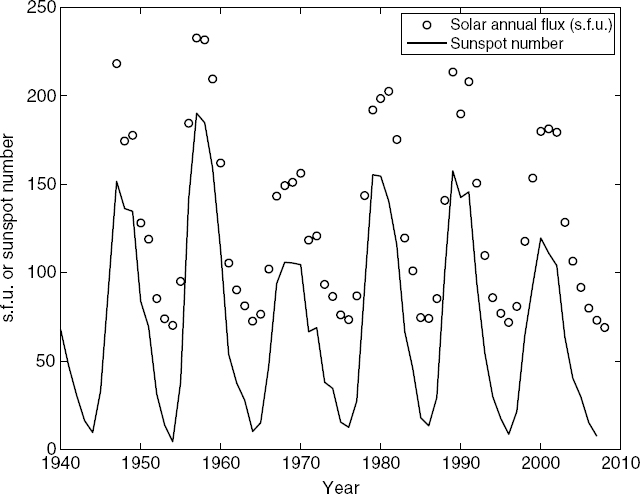
FIGURE 10.8 Time series of observed annual sunspot numbers and average annual 10.7 cm solar fluxes in solar flux units, where 1 s.f.u. = 10⁻²² W/(m² Hz).

FIGURE 10.9 Solar emission at the hydrogen alpha line (656 nm). The dark areas are sunspots. (Source: Big Bear Solar Observatory/New Jersey Institute of Technology. Printed with permission.)

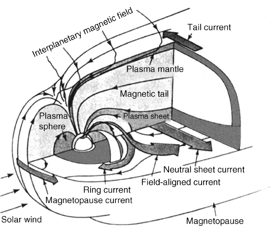
FIGURE 10.10 Illustration of the solar wind interaction with Earth's magnetic field. (Reprinted by permission from “Magnetospheric Currents,” by Thomas A. Potemra, Johns Hopkins APL Technical Digest, vol. 4, no. 4, pp. 278 (1983). Copyright Johns Hopkins University Applied Physics Laboratory.)

Streams of protons and electrons ejected from solar flares and prominences cause an increase in the solar wind. When these charged particles impact the Earth's magnetic field, they may cause a shock wave that propagates through the magnetic field, causing substantial changes and increases. Such events are called “geomagnetic storms” or “magnetic storms”. They often last for several days. When they cause major ionospheric disturbances, these are called “ionospheric storms.” Their effect on communication can be profound, but is very complicated. The mid-latitude D layer may be disturbed for more than a week. The F₂ layer electron density may increase during one phase of the storm and decrease during another. Detailed discussion of magnetic and ionospheric storms is beyond the scope of this book; the reader is referred to the literature [10].

FIGURE 10.11 Diagram of the interaction of the solar wind with the Earth magnetic field. The Sun diameter and the solar-terrestrial distance are not to the same scale as the magnetic field. (Adapted from Hunsucker, R. D., and J. K. Hargreaves, The High-Latitude Ionosphere and its Effects on Radio Propagation, p. xix, Copyright Cambridge University Press, 2003, after “Synoptic Data for Solar-Terrestrial Environment,” The Royal Society, September 1992. Reprinted with permission.)

Many of the charged particles emitted by the Sun may become trapped in the Earth's magnetic field and enter the ionosphere near the magnetic poles. This may cause an increased electron density in the D region that (as discussed in Chapter 11) can cause absorption of radio waves. When severe, this effect is called “polar cap absorption,” or PCA. PCA events may last for several days and may, at times, extend as far south as 40° latitude. Trans-polar ionospheric radio propagation becomes impossible during such events.

In addition to particle emissions, solar flares also emit strong ultraviolet and X-ray radiation. The daytime regions then show an increased electron density in the D and E regions lasting from a few minutes to a few hours with greatest intensity near the equator, where the Sun is nearly overhead. These occurrences are called “sudden ionospheric disturbances” or SIDs. The result is enhanced communication at VLF frequencies and fading, sometimes to the point of complete blackout, at HF. The reasons for these propagation effects will become apparent in Chapter 11.

Due to the important effects that solar activity has on ionospheric and trans-ionospheric propagation, several sources are available for solar activity monitoring, analysis, and forecasting, including the Space Weather Prediction Center at NOAA and the Solar Data Analysis Center at NASA.

REFERENCES

1. Rishbeth, H., “Basic physics of the ionosphere,” in Propagation of Radiowaves, second edition (L. Barclay, ed.), The Institution of Electrical Engineers, London, 2003.

2. Chapman, S., “The absorption and dissociative or ionizing effect of monochromatic radiation in an atmosphere on a rotating earth,” Proc. Phys. Soc., vol. 43, pp. 26–45, 1931.

3. Davies, K., Ionospheric Radio Propagation, National Bureau of Standards Monograph 80, U.S. Department of Commerce, 1965.

4. U.S. Standard Atmosphere, National Oceanic and Atmospheric Administration, Washington, DC 1976.

5. Reinisch B., and D. Bilitza, “Karl Rawer's life and the history of IRI,” Adv. Space Res., vol. 34, no. 9, pp. 1845–1950, 2004.

6. Bilitza D., and B. Reinisch, “International Reference Ionosphere 2007: improvements and new parameters,” Adv. Space Res., vol. 42, no. 4, pp. 599–609, 2007.

7. Hochegger, G., B. Nava, S.M. Radicella, and R. Leitinger, “A family of ionospheric models for different uses,” Phys. Chem. Earth, vol. 25, no. 4, pp. 307–310, 2000.

8. ITU-R Recommendation P.531-9, “Ionospheric propagation data and prediction methods required for the design of satellite services,” International Telecommunication Union, 2007.

9. Fritts D. C., et al., “Overview and summary of the Spread F experiment (SpreadFEx),” Ann. Geophys., vol. 27, pp. 2141-2151, 2009.

10. Hargreaves, J. K., The Solar-Terrestrial Environment: An Introduction to Geospace—The Science of the Terrestrial Upper Atmosphere, Ionosphere, and Magnetosphere, Cambridge University Press, Cambridge, 1992.