2

CHARACTERIZATION OF PROPAGATION MEDIA

2.1 INTRODUCTION

It is assumed that the reader has some familiarity with electromagnetic field theory and has encountered plane waves before. Nevertheless, a brief review here seems appropriate because introductory treatments, particularly for engineers, often steer quickly toward the simplest dielectric and magnetic materials. This simplifies the equations and allows an early introduction to waveguides, antennas, and other applications. Propagation media are not necessarily simple, however, and departure from the simple model can strongly impact signal propagation.

2.2 MAXWELL'S EQUATIONS, BOUNDARY CONDITIONS, AND CONTINUITY

The starting point for electromagnetic theory [1–5] is the set of four equations named after James Clerk Maxwell:

In these equations, the overbars denote vectors, t represents time, and the usual notation of vector calculus is used. denotes the magnetic field intensity (A/m), the magnetic flux density or induction (T), the electric field intensity (V/m), the electric flux density or induction (C/m²), ρ the volume density of free charge (C/m³), and the current flow density due to free charges (A/m²).

From these equations some auxiliary relations can be deduced. Among these are the boundary conditions, which hold at the interface of any two regions of space:

Here denotes a unit vector normal to the interface and pointing out of region 1 into region 2 (see Figure 2.1), the subscripts indicate the regions in which the fields are to be evaluated at the boundary, denotes the surface current density, and ρ_S denotes surface charge density on the boundary between the regions. These boundary conditions are very useful when problems involving several materials are considered: Maxwell's equations can then be solved in each homogeneous region and the resulting solutions matched by applying the proper boundary conditions across the interfaces. This usefulness should not obscure the fact that the above boundary conditions add no real information to the Maxwell's equations: by assuming finite amplitude fields, equation (2.5) can be deduced from (2.1), (2.6) from (2.2), and so on. A similarly useful, but also dependent set of equations are the charge continuity equations

FIGURE 2.1 Unit vector at boundary of two regions.

Equation (2.9) results when the divergence of both sides of equation (2.1) is taken; the left-hand side can then be shown to be zero by a vector identity, and by application of equation (2.3) to the right-hand side, equation (2.9) can be obtained. Equation (2.10) can be obtained from equation (2.9) by considering current flow parallel to a boundary surface in a boundary region of vanishingly small thickness. The continuity equations are very useful because they express an important physical concept that a net outflow of current from a region depletes the free charge within that region (charge conservation); in short, that current is the flow of charge. Again, the importance of that concept should not obscure the fact that the continuity equations follow from Maxwell's equations.

2.3 CONSTITUTIVE RELATIONS

Maxwell's equations by themselves are not sufficient to specify a problem. From the mathematical point of view, the Helmholtz theorem states that it is necessary to specify both the divergence and curl of a vector to determine its departure from a constant vector. Maxwell's equations deal with two electric vectors, and , but specify only the curl of one and the divergence of the other. Without a relationship between the two, there is insufficient information about either. The same is true for the magnetic field vectors and . From a physical point of view, Maxwell's equations by themselves must be incomplete because they take no account of the material medium in which they are considered. Experimentally, one finds that the material has a very pronounced effect on the fields. In fact, practical problems are often specified by giving (a) the material properties and (b) the field values at the boundary of the region of interest.

The equations that, mathematically, link the various field vectors and, physically, account for the effects of a material medium are called constitutive relations. For particularly simple materials, the link is very convenient and direct:

where ∈ is the permittivity and μ the permeability of the material. Equations (2.11) and (2.12) are, however, based on a host of assumptions that are often not satisfied in propagation media. It is therefore worthwhile to go back to a more basic set of relationships to examine the nature of the constitutive equations.

2.4 DIELECTRIC BEHAVIOR OF MATERIALS: MATERIAL POLARIZATION

According to the atomic theory, matter is composed of atoms consisting of positively charged nuclei and orbiting electrons. The atoms combine to form molecules; in liquids and solids, these may, in turn, be arranged into more complex structures. The separation between each orbiting electron and the corresponding positive nuclear charge causes these charges to constitute an electric dipole (an electric dipole is an equal amount of positive and negative charge separated by a small distance). Thermal motions cause a constant reorientation of these dipoles, and under many conditions the orientation of the dipoles is completely random; the average dipole moment per unit volume is then zero. This average dipole moment per unit volume is called the polarization vector , where the average is to be taken over a volume surrounding the point (x, y, z) small enough to be associated with a point as far as field calculations are concerned, but large enough to contain many molecules, or other ordered structures (such as crystals). No specific coordinate system is implied, and we will write instead of to emphasize this point. In the presence of an externally applied electric field (and even without such a field in the case of ferroelectric materials), some order is injected into the randomness of the dipole orientation and in that case the polarization vector, , which represents the average dipole moment per unit volume, assumes nonzero values. The electric flux density is then related to the actually existing electric field intensity by the relation

where the first term on the right-hand side represents the flux corresponding to the same electric field intensity in free space (vacuum, with permittivity ∈₀ = 8.854 × 10⁻¹² F/m), and the second term represents the contribution of the polarization, that is, the effect of the material. Of course, the electric field due to a given set of sources (charges) in the presence of the dielectric is different from what it would be in free space. Equation (2.13) is the generalization from which equation (2.11) can be derived, but only for very simple materials. Two words of caution may be appropriate at this point. First, the electric field intensity in equation (2.13) is the actual macroscopic field that exists in the material, not the applied field that would exist in the absence of the material. This is unfortunate because the actual field is not always easy to calculate. Second, the polarization of a material, which is under discussion here, should not be confused with the polarization of a wave, which will be discussed later. It is unfortunate that the same word is used for two different concepts, and we need to be careful to distinguish between material polarization and wave polarization in contexts where confusion might arise.

Equation (2.13), while more general than equation (2.11), is not as effective in providing, together with Maxwell's equations, a complete set of equations for the description of electromagnetic phenomena. The reason is that we have added not only an equation but also an additional vector, . We must bring in now the relation between and , which depends on the material. For particular materials the relationship can be quite simple, but for others it can be very complicated. Let us look briefly and qualitatively at the complicating properties.

2.5 MATERIAL PROPERTIES

Nonlinearity When the applied field strength is sufficiently low, as is generally true in typical propagation problems, the three components of the polarization vector depend in some linear fashion on the three components of the electric field intensity . This characterizes linear media. Since linear differential equations are much easier to solve than nonlinear ones, this is a great simplification. However, if the fields are strong enough, the approximation breaks down. For example, linear optical propagation theory is not a valid theory for a high-powered focused laser propagating in air at normal pressures, because such a beam will produce significant ionization and hence nonlinear effects.

Anisotropy Most media have no directional properties of their own. In such a medium, each component of depends only on the corresponding component of , and the dependence is the same for all components. This greatly simplifies the relationship, although it does not guarantee that and have the same direction at all instants of time. (For example, in a dispersive medium (see below) if the direction of changes, the vector cannot follow that direction change instantly.) Media that have no directional properties of their own are called isotropic; those that do are called anisotropic. The ionosphere is an example of an anisotropic medium since the Earth's magnetic field gives some directionality to the motions of charges in it. Therefore, in the ionosphere, equation (2.11) is invalid (except in a very approximate sense) and equation (2.13) will need to be used. All other media considered in this text are isotropic.

Dispersion The material polarization is the result of a statistical alignment or orientation of the charge dipoles in a medium, counteracted in part by the constant disordering influence of thermal motion. This alignment cannot occur instantaneously, and neither can the disordering after the applied field is removed. For many materials, the ordering process is much faster than the disordering process, and disordering can be characterized approximately by an exponential function. The time constant of this function is then called the relaxation time of the polarization. When the applied signal varies slowly with respect to the ordering and disordering processes, the polarization appears to follow the applied field almost instantaneously. In that case, to find the polarization at a given time, we need to know only the instantaneous applied field at that same time. On the other hand, if the signal varies significantly within the time required for ordering and disordering to take place, the polarization effects lag behind the applied field that causes them. Then we need to know the prior time history of the applied field to find the polarization at any given time. In this case, the rate of variation of the signal becomes important, hence different frequencies will produce different polarization responses. A medium whose response depends on the frequency is called dispersive, otherwise it is called nondispersive. From the foregoing discussion it should be apparent that most materials exhibit nondispersive properties up to some frequency regime characteristic of the polarization process involved and hence the particular material. They will act dispersively at frequencies close to that regime. At sufficiently high frequencies (i.e., those much higher than the reciprocal of all the characteristic times of the ordering–disordering process), the polarization charges will be unable to follow the field variations at all, and the material will exhibit the dielectric properties of free space.

Inhomogeneity and Time Dependence The dielectric properties of a medium may be the same at every point within the medium or they may vary from place to place. In the first case, the medium is called homogeneous; in the second, inhomogeneous. The properties may also be invariant with time or time-dependent. In natural propagation media, inhomogeneities are often associated with time variation. For example, tropospheric inhomogeneities, which make possible the tropospheric scatter mechanism, drift with winds and change in size and shape with time.

Fortunately, not all the complicating properties discussed above need to be considered simultaneously. For most problems, it is only necessary to consider one or two of them, but even then the resulting solutions of Maxwell's equations become complicated. The relationship between the electric flux density and the electric field intensity for some relatively simple media of practical relevance for propagation problems will be considered in the next several sections.

2.5.1 Simple Media

The Simplest Medium Consider first the simplest possible dielectric media, namely, those that are isotropic, linear, homogeneous, time-invariant, and nondispersive. The last property is a restriction on the rate of change of the applied signal as well as on the material properties, as discussed previously. For such a medium, the relationship between and can be written as

The constant χ is called the electric susceptibility of the medium. Clearly, equation (2.14) is linear. Furthermore, each component of depends only on the corresponding component of and all have the same proportionality constant, satisfying the isotropic assumption. At any time, the polarization depends only on the field intensity at that same moment satisfying the nondispersive assumption. Since χ is independent of position or time, the medium is also homogeneous and time-invariant. This is the simplest relationship between and that a material can exhibit. Use of equation (2.14) in equation (2.13) gives

where

and

The constant ∈_r is called the relative dielectric constant or the relative permittivity.

Simple Inhomogeneous and Time-Varying Media The word “simple” will be used to describe a medium that has properties identical to the simplest medium just discussed, with the exception of those specifically mentioned in the name. Thus, “simple inhomogeneous and time-varying media” are isotropic, linear, and dispersionless, by definition. Allowing inhomogeneity and time variation has, indeed, a very simple effect on the constitutive relations, which become

so

The “simplicity” ceases at this point, however, because solutions of Maxwell's equations in conjunction with (2.19) are generally much more difficult than when ∈ is a constant.

Simple Dispersive Media As mentioned before, a medium acts dispersively when the characteristic relaxation times are comparable to the rate of change of the impressed electric field. Under these conditions, the polarization is unable to follow the field instantaneously.

The polarization vector arises from an average displacement of charges from their statistically neutral positions. Each charge individually obeys an equation of motion with respect to the electric field intensity. If one assumes that all forces except those due to the field are local (on a macroscopic scale), these equations are ordinary differential equations; then the relationship between the polarization and the electric field intensity is also an ordinary differential equation with time as the independent variable. Assuming the material is isotropic, we can consider each of the field components separately. For example, we have for the x components

where is a differential operator involving differentiation with respect to t only. Since the material is to be simple except for dispersion, we have ruled out nonlinear or time-varying constitutive effects. As a result, we can assume that the operator is linear with constant coefficients. The solution for P_x(t) can be written as a superposition integral

where f_I(t) is the impulse response of the medium. Since the “simple” dispersive medium under discussion is assumed isotropic, similar equations may be written for the y and z components, so a more general equation is

The limits in the above integral imply causality: the electric field for −∞ < t′ <t influences the behavior of at time t, while the electric field for t′ > t does not. In other words, only the past history of the electric field determines the polarization at any instant of time.

The above considerations have been mostly heuristic. Moreover, a classical model has been assumed, whereas one might argue that in the discussion of microscopic phenomena, a quantum model would have been more accurate. Actually, when the problem is formulated quantum mechanically, one finds that summing over all allowed quantized orientations is equivalent, as far as the final results are concerned, to the classical model integration over a random orientation of orbits.

In many cases, the polarization function f_I(t) can be approximated for t > 0 by a sum of the form

where the time constants τ_i are the relaxation times of the individual polarization processes. Since f_I(t − t′) characterizes the polarization at time t due to an electric field impulse at t′, and since random thermal motion operates to disorder the polarized molecules, f_I(t − t′) approaches zero for t t′. If the electric field is static, or if the electric field is so slowly varying that remains essentially constant over the time interval over which f_I(t − t′) is much different from zero, then may be taken out of the integral to yield

This leads to the electrostatic or quasi-static representation

where the last equality results from letting t − t′ = ζ.

The dielectric constant for the electrostatic or quasi-static case then becomes

This representation is valid for all materials that are polarized entirely by electronic and atomic alignments up to the submillimeter wave region; however, for materials that exhibit molecular (Debye) or interfacial polarization effects, equation (2.22) must be used for radio waves.

So far we have considered polarization as related to an arbitrary time-varying electric field. The assumption of sinusoidal (time-harmonic) time dependence greatly simplifies the analysis, and this assumption will be very useful in much of the material to be covered in this book. If we express a sinusoidal field in equation (2.22) by the usual phasor representation

where is the radian frequency of the sinusoidal field, and the underbar denotes a complex number, one gets from equation (2.22)

Again letting t − t′ = ζ gives

Letting

one gets

where

The last equation defines the complex susceptibility (ω).

It can be shown easily that equations (2.32) and (2.13) lead to a complex dielectric constant, or complex permittivity,

which can be related to the fields by

where

is implied. It is also easy to show that the complex susceptibility and complex dielectric constant approach the quasi-static values as ω approaches zero.

The appearance of equation (2.34) is deceptively similar to that of equation (2.15),

that applies to the quasi-static case (and hence to the simplest media, since a simple dispersive medium reduces to that when the quasi-static assumption is satisfied). However, they are really quite different in meaning. In equation (2.15), ∈ is a real constant relating the arbitrarily time-varying vectors and . In contrast, ∈(ω) in equation (2.34) is a complex function of ω that relates the phasor representations of and , for sinusoidal time variations.

The imaginary part of ∈(ω) can be shown to result in a loss of energy in the material. This phenomenon occurs because lags , and it is called dielectric hysteresis loss. The most general behavior of the complex dielectric constant of a material is shown in Figure 2.2. In this figure, the legends refer to four different polarization mechanisms corresponding to progressively longer relaxation times. At the lowest frequencies, all are effective and the complex dielectric constant is essentially real and large. As the frequency ω is raised to a value such that the period T = 2π/ω is on the order of the relaxation time τ of the interfacial polarization process, the dipoles corresponding to that process can no longer follow and the dielectric constant due to that process begins to disappear. In this region, the lagging dipole moments cause an increase in dielectric hysteresis loss that shows up as a hump in the imaginary part of ∈. The same behavior is observed for the other polarization mechanisms. Not all materials exhibit all the polarization mechanisms: the dispersion curves for water, which exhibits molecular polarization, and carbon tetrachloride, which has only atomic and electronic polarization, are shown in Figures 2.3. One can notice that there is a correlation between variations in the real part of the permittivity ∈′ and the value of the imaginary part of the permittivity ∈″. Indeed, ∈′ and ∈″ are related by the so-called Kramers–Kronig relations. The details of Figures 2.2 and 2.3 are not important to our discussion here. The important concepts to remember are that the dielectric constant can vary considerably with frequency, and so can the dielectric loss.

FIGURE 2.2 Schematic representation of complex dielectric constant variation.

At this point, let us summarize the important points about the dispersive characteristics of materials otherwise simple. Simple relations of the type

are not valid unless the applied electric field is slowly varying compared to the ordering–disordering processes responsible for polarization, a condition we have called quasi-static. The more general relation takes the form

FIGURE 2.3 Dielectric behavior at 25°C (a) distilled water and (b) carbon tetrachloride.

and susceptibility and dielectric constant cannot be defined for arbitrary time variation. When the excitation is sinusoidal, however, equation (2.22) can be converted to a relation between the phasors that characterize and , namely, equation (2.31), and hence equation (2.34) follows. The complex susceptibility and complex dielectric constant that appear in these equations are functions of frequency, and their imaginary part corresponds to a dielectric hysteresis loss.

A distinction should also be made here between the dispersive properties of a dielectric material, which have been discussed here, and the dispersive properties of an entire signal path of which the material may be only a part. Consider, for example, a slab of the “simplest material”, which in itself has no dispersion, and let a wave be normally incident upon it. The surrounding medium is free space. It will be found that there is no reflection if the frequency is chosen so that the thickness of the slab is a precise multiple of half-wavelengths, but at other frequencies there will be reflections. Clearly, the path is dispersive, since it does not treat all frequencies alike, even though the material in the slab is not a dispersive material.

Simple Anisotropic Media An anisotropic material exhibits certain preferential polarization directions. As a result, the polarization does not necessarily align itself with the electric field. Thus, it is no longer true that the x component of responds only to the x component of and so forth, although such simple relations may still hold in special coordinate systems. In general, we must write

which can be abbreviated symbolically as

The elements χ_ij of the susceptibility matrix [χ] are not all independent, and the matrix can often be simplified considerably by taking advantage of the symmetries that occur when coordinate axes are chosen to coincide with symmetry axes of the material. These details need not concern us here; for the moment we wish to stress only that the simple relation of equation (2.14) must be replaced by the matrix relation (2.37) in the case of anisotropic materials. The corresponding relationships between and follow from equation (2.13),

which may be written as

where

in which [I] represents the identity matrix,

Simple Nonlinear Media In nonlinear media, the polarization is no longer linearly related to the electric field intensity. In an otherwise simple nonlinear medium, the most general relationship is

The first of these equations states that the directions of and are same, the â's denoting unit vectors of the respective field directions. The second equation leaves the relationship between their magnitudes quite general. Often, it is possible to expand the magnitude function f_N in a Taylor series, to obtain

and to neglect higher order terms. The electric field strength that must be exceeded before a given material becomes noticeably nonlinear is a property of the material and varies greatly from one medium to another. For the media prevalent in radiowave propagation, the required field strengths are usually quite high, and it is unusual to consider nonlinear effects. An exception is the propagation of very high powered waves in the ionosphere, in which case the nonlinearity can produce an intermodulation of signals, the so-called “Luxembourg effect”. Another exception is the parametric generation of coherent light in a nonlinear propagation path. In general, nonlinear phenomena are likely to become more important in optical propagation because of the very high local field strengths that can be achieved with lasers. Nonlinear effects are not considered further in this book.

More Complicated Media Any number of the properties seen above—nonlinearity, anisotropy, dispersion, inhomogeneity, time variability—can, of course, sometimes coexist in a propagation medium. In many cases, the extension from the simple media described above is conceptually straightforward, but the solution of Maxwell's equations becomes increasingly difficult in more complicated media. For example, the ionosphere must be treated in some calculations as an anisotropic, dispersive, and inhomogeneous medium. From the discussion of simple dispersive media, we know that we should not expect to derive real susceptibilities or real dielectric constants, valid for arbitrary time dependence, but should look for complex quantities relating the phasors corresponding to and or and . From the discussion of simple anisotropic media, we seek not single constants but a matrix to relate the components. From the discussion of simple inhomogeneous media, we expect the matrix elements to be functions of position. Indeed, relationships of the form

turn out to be appropriate for the ionosphere, where

Time variations of the form of equation (2.27) are understood, and the [χ] and [∈] matrices differ from those in equations (2.37) and (2.39) in that each element is complex and a function of position and frequency.

There are some cases, however, where the treatment of complicated media is difficult even at a conceptual level. These arise primarily when nonlinearity occurs in conjunction with dispersion or anisotropy. Linearity played an important role in the discussion of the simple dispersive and simple anisotropic medium, but there is no simple way to generalize these treatments to the nonlinear case. We note that there is great current interest in the production of engineered “metamaterials” to achieve greater control over constitutive relations for fabricating new electromagnetic devices.

2.6 MAGNETIC AND CONDUCTIVE BEHAVIOR OF MATERIALS

Just as the dielectric behavior of materials can be very simple or very complicated, so can their magnetic and conductive behavior. For propagation problems, it is seldom necessary to consider materials that exhibit strong magnetic effects. For all the propagation mechanisms considered in this book, the simple, free-space relation

is valid with sufficient accuracy, where μ₀ = 4π × 10⁻⁷ H/m is the permeability of free space.

Conductive behavior does occur in propagation problems, for example in the ionosphere and in the ground. The same complicating characteristics (nonlinearity, anisotropy, etc.) that came up in connection with dielectrics occur in regard to conductivity as well. The analogy is so direct that it would be repetitious to examine conductive behavior in great detail. For example, in direct analogy with equation (2.14), the simplest conductive behavior is characterized by

where is the current density and σ (S/m or mho/m) is the conductivity of the material.

For a simple anisotropic conduction process, one has in analogy with equation (2.39)

where

The other analogies should be obvious.

2.6.1 Equivalence of Ohmic and Polarization Losses

Consider a medium in which conduction by free charges can take place; the medium also exhibits simple dispersive polarization. Because of the dispersive nature of the polarization, it is easiest to deal with the phasor representations of the fields. Letting

and similarly for and , one gets for equation (2.1),

and by equations (2.34) and (2.50)

If one separates out the real and imaginary parts of the dielectric constant,

and rearranges the terms slightly, the result is

The σ term in this last equation represents conduction current due to free charges and results in ohmic loss. The term represents lagging polarization, producing an effective current in phase with the conduction current. It is responsible for the polarization hysteresis loss. The effects of these two losses on a signal propagating through a medium are same; indeed, it is not easy to design an experiment for measuring them separately. At a first glance, from equation (2.57) it might appear that the frequency dependence of the polarization term would make it easy to separate the two, but this is not so since in the dispersive material σ and ∈″ themselves are frequency dependent. In any case, from the propagation point of view there is no need to separate the two effects, and generally they are lumped together.

For this purpose, two representations are commonly employed. The first, commonly used to specify the ground properties at MF (e.g., the U.S. AM broadcast band), is based upon lumping the two terms into an effective conductivity,

Defining the relative dielectric constant

and a loss factor

Ampere's law becomes

The quantity (∈_r − jx) appears frequently in calculations. A handy formula for computing x is

where σ_e is measured in mho/m and f in MHz. The subscript “e” on σ_e is often omitted; whenever a real dielectric constant and conductivity are specified for a lossy dielectric, such as ground, it is safe to assume that the effective conductivity is meant.

A second convention, used especially at microwave frequencies, is based upon representing the material as though polarization accounted for all the losses. In this case, an effective imaginary dielectric constant is introduced as

and a loss tangent as

so Ampere's law becomes

The term “loss tangent” is derived from representing the dielectric constant as a complex number

as in Figure 2.4. Under this convention, too, it is usual to omit the subscript denoting “effective”; whenever the dielectric behavior is specified by ∈′ and ∈″ or tan δ, it is safe to assume that conductivity effects are also included.

It is sometimes necessary to convert between the two representations. By equating the right-hand sides of equations (2.61) and (2.65), one finds

Figure 2.5 provides a plot of dielectric constant and conductivity values for various soils and ocean water, from ITU-R Recommendation 527-3 [6]. A map of the ground conductivity of the continental United States (in millimhos per meter) from ITU-R Recommendation 832-2 “World Atlas of Ground Conductivities” [7] is shown in Figure 2.6. It was compiled for use in the U.S. AM broadcast band, 540–1600 kHz. The real part of the relative dielectric constant ∈_r also varies with soil type, but not over as wide a range.

FIGURE 2.4 Loss tangent diagram.

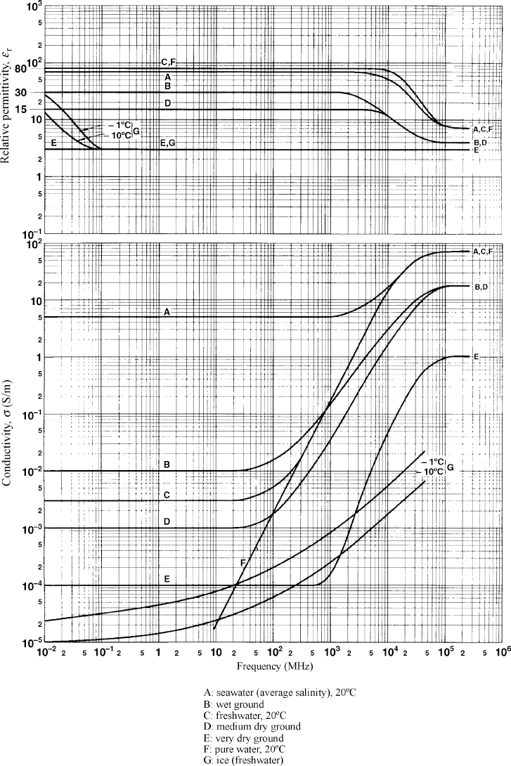
FIGURE 2.5 Dielectric constant and conductivity values for several natural materials versus frequency. (Source: ITU-R Recommendation 527-3, used with permission). The convention of (2.58) and (2.59) is implied.

FIGURE 2.6 Ground conductivity (millimhos per meter) in the United States. (Source: ITUR Recommendation 832-2, used with permission). The convention of (2.58) is implied.

REFERENCES

1. Stratton, J. A., Electromagnetic Theory, Wiley–IEEE Press, 2007.

2. Kong, J. A., Electromagnetic Wave Theory, EMW Publishing, 2008.

3. Harrington, R. F., Time-Harmonic Electromagnetic Fields, McGraw-Hill, 1961.

4. Chew, W. C., Waves and Fields in Inhomogeneous Media, IEEE Press, 1999.

5. Landau, L. D., L. P. Pitaevskii, and E. M. Lifshitz, Electrodynamics of Continuous Media, second edition, Butterworth-Heinemann, 1984.

6. ITU-R Recommendation P.527-3, “Electrical characteristics of the surface of the Earth,” International Telecommunication Union, 1992.

7. ITU-R Recommendation P.832-2, “World Atlas of Ground Conductivities,” International Telecommunication Union, 1999.