7

TERRAIN REFLECTION AND DIFFRACTION

7.1 INTRODUCTION

In many applications, line-of-sight communications are influenced by reflections from the surface of the Earth. Transmitting and receiving paths near the surface of the Earth will experience reflections from the ground if sufficient antenna directivity is not available to avoid ground illumination. Examples include VHF and UHF broadcast systems where receivers (such as radio and television antennas) are located near the ground surface, preventing its influence from being removed even with large transmitting antenna heights.

In this chapter, the theory of direct plus reflected wave propagation is presented, along with a graphical method for predicting propagation effects in the presence of irregular terrain. This chapter provides a first discussion of “multipath” interference for the simple case of a single multipath (reflection from the ground surface). Multipath propagation effects are further examined from an empirical and statistical point of view in Chapter 8. In addition, a rule of thumb for siting antennas in point-to-point links to avoid obstruction of the line of sight by terrain is presented. The latter is “site specific” in that the focus is on situations where the terrain elevation is known as a function of distance from the transmitter and the receiver. Empirical models for propagation loss in cases where the terrain is not specified (as for a mobile communication system) are dealt with in Chapter 8. Because the obstruction considered here is the Earth's surface itself, the discussion applies mainly to nonurban environments; the influence of buildings, vehicles, and other such “clutter” objects is not considered.

7.2 PROPAGATION OVER A PLANE EARTH

For terrain that is relatively smooth on a wavelength scale, the surface of the Earth may be approximated as a dielectric plane at sufficiently short distances where Earth curvature effects are negligible. In this situation, a transmitting antenna with finite directivity illuminates both the receiving antenna and a portion of the ground surface, so that the receiver receives a direct and a specularly reflected signal, as discussed in Chapter 6. Figure 7.1 illustrates the geometry of this situation, from which the following geometrical relationships can be derived:

where ψ₁ and ψ₂ refer to the declination angles along the direct and reflected paths R₁ and , respectively. Note that the reflected wave can be interpreted as arising from an “image” of the true source that is located a distance h₁ below the Earth's surface. The reflected wave contributed by the image source is computed as if the image source were in free space, except that the field is multiplied by the reflection coefficient encountered on the true reflected wave path.

Throughout the following, we will assume that the receiver is in the far field of both the true and image sources and that the horizontal distance d between the two antennas is much larger than either of the antenna heights.

FIGURE 7.1 Geometry for reflection problem.

7.2.1 Field Received Along Path R₁: The Direct Ray

From equation (5.2), assuming impedance and polarization matching and no atmospheric attenuation, the power density of the direct ray, if it existed alone, would be

where P_T is the power transmitted and G_T is the transmitter gain in the direction of the receiving antenna. From this and

where η is the characteristic impedance of free space and peak values are used for the field amplitude, we can obtain

so

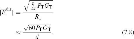
where the latter equation substitutes η ≈ 120π ohms. In equation (7.8), if is to be in volts/meter, P_T must be in watts and d in meters. In the literature, equation (7.8) is often written as

where

and

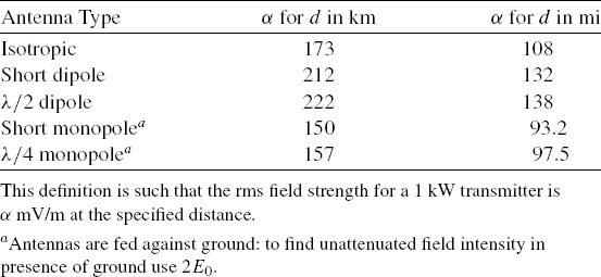
E₀ is called the “unattenuated field intensity at unit distance” and is usually specified in mV/m at 1 km with the understanding that the distance d is then specified in km. From equation (7.10), E₀ depends only on the transmitted power (usually measured in kW) and α, which in turn depends only on the transmitter antenna gain G_T. Using the standard units (mV/m at 1 km for E₀ and kW for P_T), values of α can be tabulated; examples for common antennas are given in Table 7.1. Values using mV/m at 1 mile units for E₀ are also provided.

TABLE 7.1 Values for α so That E₀ in mV/m at Specified Distance with P_T in kW

7.2.2 Field Received Along Path R₂: The Reflected Ray

The magnitude of the reflected ray can be calculated similarly except for the reflection process. The plane wave reflection coefficients from Chapter 6 may be used to obtain

where R₂ ≈ d has been used in the denominator, and it has also been assumed that the antenna gain is identical along the direct and reflect ray paths so that E₀ is the same for both. Γ is to be taken as either Γ_|| or Γ_⊥ depending on the polarization utilized; for ground-to-ground station propagation problems, both reflection coefficients are near −1 due to the small declination angles involved.

7.2.3 Total Field

The total field is obtained by adding the direct and reflected fields in the proper phase relationship,

where is the phase constant in free space. Though correct, this relationship is not in a useful form since k₀R₁ and k₀R₂ are generally many thousands or millions of radians and Γ is often near −1,¹ therefore great precision would have to be used in evaluating the exponentials. Instead, use

to obtain

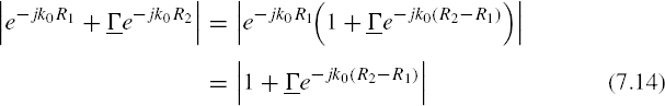
From the geometry,

and use of the binomial theorem for x >> y gives

Similarly,

so that

a generally important and useful relationship for antennas located much further from one another than their heights above the ground.

Use of this in equation (7.15) gives

This is the relationship that normally should be used to calculate the field. If the heights are small, the reflection coefficient approaches −1 and the exponential may be replaced by the first two terms of its Maclaurin's series expansion, 1 − j2k₀h₁h₂/d, to give

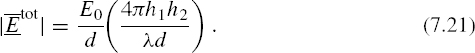
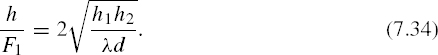
The factor in parenthesis is dimensionless, and any consistent units may be used in it. Equation (7.21) is applicable only for cases where 2k₀h₁h₂/d is less than approximately 0.5; this condition can be rewritten as

with h₁ and h₂ in meters. When applicable, equation (7.21) shows that the received field decays as one over the distance squared, as opposed to the one over distance decay in free space. This more rapid loss of field intensity is caused by destructive interference between the direct and reflected rays.

Equation (7.20) provides our first specific example of “multipath” in that the total received field consists of contributions from waves that have different phases due to their differing path lengths. Since the total field amplitude is proportional to the sum of two numbers, 1 and Γe^{−j2k₀h₁h₂/d}, the constructive or destructive interference of these terms depends on their relative phases. In situations where Γ ≈ −1, the two terms have identical amplitudes, and the total field amplitude can vary from zero to twice that of the direct ray.

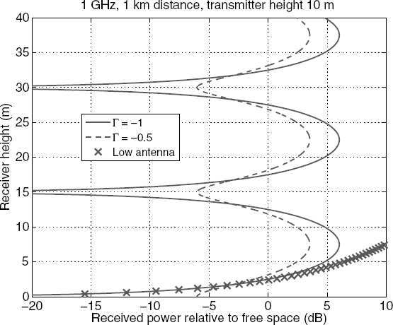
FIGURE 7.2 Height-gain curve example: received power relative to free space in dB as the receiver height is varied: 1 GHz, 1 km distance between antennas, and transmitter height 10 m. Results using Γ = −1, Γ = −0.5, and equation (7.21) are compared.

7.2.4 Height-Gain Curves

A quantity of interest in many propagation applications is a “height-gain curve”: this is a plot of the received power as either the receiver or the transmitter height is varied at a fixed separation. It is common to scale such plots by the power that would have been received if the direct ray alone were present, in this case the power associated with E₀/d. The quantity is thus the “received power relative to the power that would be received in free space,” typically presented in decibels. Figure 7.2 plots this quantity on the horizontal axis versus the receiving antenna height on the vertical axis (a common practice with height-gain curves) for a 1 GHz transmitter frequency, a 1 km separation between the antennas, and a 10 m transmitter height. Curves are included for Γ = −1, Γ = −0.5, and the simplified form in equation (7.21). The results show an oscillation of the received power as a function of receiver height due to the changing phase difference between the direct and reflected rays as the receiver height varies. For Γ = −1, the nulls in the oscillation approach minus infinity decibels since zero field strength can occur in this case, while the maxima are at 6 dB since this represents a doubled field strength. The oscillation is smaller for Γ = −0.5 since complete constructive or destructive interference does not occur in this case. Finally, the linear increase in field amplitudes (quadratic increase in power) with receiver height predicted by equation (7.21) holds only for portions of the height-gain curve significantly below the first maximum. It is of course desirable in establishing point-to-point links to avoid destructive multipath interference; this issue will be discussed further later in the chapter.

FIGURE 7.3 Received power relative to free space in dB as a function of distance: 1 GHz, transmitter and receiver heights of 10 m. Results using Γ = −1, Γ = −0.5, and equation (7.21) are compared.

Similar effects can be observed in the received power versus range for fixed transmitter and receiver heights (Figure 7.3). Since the phase difference varies inversely with the distance, more rapid oscillations are observed at shorter ranges that eventually resolve into a slow decay as the fourth power of distance when equation (7.21) is applicable. It would be more likely in practice to consider height-gain curves at a fixed distance (as in Figure 7.2) when considering sites for point-to-point systems, while an examination of propagation losses versus range (as in Figure 7.3) would be more appropriate for airborne communications or radar applications.

7.3 FRESNEL ZONES

The discussion of the previous section has considered the direct and specularly reflected rays for propagation over a planar surface. For nonplanar surfaces, it is also of interest to consider the impact of reflections from other surface points. Signals arriving through these reflected rays would be delayed compared to the direct ray. To be delayed by n × 180°, the path via reflection must exceed the direct path length by nλ/2, where λ is the wavelength.

The set of points at which reflection would produce an excess path length of precisely nλ/2 is called the nth Fresnel zone. From analytic geometry, it is known that in a plane this collection is an ellipse; in three-dimensional space, it is an ellipsoid of revolution with the direct ray as its axis. The diameter of the ellipsoid increases with increasing n, as sketched in Figure 7.4. While reflections can occur anywhere around the path, most good reflecting surfaces are horizontal, and it is therefore usually sufficient to consider only the vertical plane containing the direct ray.

A signal arriving via reflection from the first Fresnel zone suffers a 180° phase shift at the reflection point (since Γ_⊥ or Γ_|| ≈ −1 for grazing incidence) and another 180° phase shift by virtue of its λ/2 excess path. It will therefore reinforce the direct ray and produce a maximum. A signal arriving via reflection from the second Fresnel zone suffers a 180° phase shift at the reflection point and a 360° phase shift due to excess path; it will therefore cancel the direct ray. In similar manner, all odd Fresnel zone reflections produce maxima and all even Fresnel zone reflections produce minima. A convenient formula for calculating the radius of the nth Fresnel zone at a distance d₁ from one end of the path is

FIGURE 7.4 Fresnel ellipsoids.

where F_n is the radius of the nth Fresnel zone in m for a path of length d at a distance d₁ from one end of the path, d₂ from the other end, all in km, at a frequency given by f in GHz. This formula can be derived as follows:

Let AB be the direct path and ACB the path via the reflection point C as shown in Figure 7.5. The condition that will locate C on the nth Fresnel zone is

FIGURE 7.5 Triangle for calculation of Fresnel zones.

where λ is the wavelength and the other dimensions are as defined in Figure 7.5. Using the right triangle relations gives

The distance AB is on the order tens of km while F_n will turn out to be on the order of tens of meters; therefore, except right near the end points A or B, we can expand the square roots by the binomial theorem and retain only the first two terms since :

Therefore,

Using d = d₁ + d₂, we get

where F_n, λ, d₁, d₂, and d are all in the same units. Use of λ = c/f and conversion of units gives equation (7.23). Note that the Fresnel zone radii scale directly with and with , and are therefore larger at lower frequencies.

Figure 7.6 is a plot of the Fresnel zone radii at 3.95 GHz versus distance along a 20 km path and shows an increase from zero at the transmitting and receiving locations to a maximum at the middle of the path.

In practice, complete cancelation and reinforcement (Γ_⊥ or Γ_|| = −1) occur only for very smooth surfaces such as lakes, tennis courts, paved roads, and so on. For rough surfaces (i.e., surfaces whose roughness is an appreciable part of a wavelength), the effective reflection coefficient amplitude varies between zero and −1.

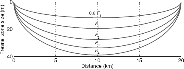
FIGURE 7.6 Variation in 3.95 GHz Fresnel zone radii along a 20 km path.

7.3.1 Propagation Over a Plane Earth Revisited in Terms of Fresnel Zones

Propagation over a plane Earth provides an interesting example for using Fresnel zones to interpret reflections, since there is only a single reflection point from the terrain and the location of this reflection point is known. Referring to Figure 7.1, the reflection point on the planar surface is located at the distance d₁ = d_r, where a line drawn from the image source to the receiver intersects the ground surface (height zero), that is,

or

The direct ray can be represented by a line whose height above the ground surface is

which for d₁ = d_r yields a reflection point clearance h of

It is of interest to compare the height of the direct ray above the reflection point with the Fresnel zone radii at the location of the reflection point. The latter are

Combining equations (7.32) and (7.33), we obtain

When h/F₁ is unity, constructive interference will occur; when , destructive interference will occur, and so on. It can also be shown that the value of h/F₁ in equation (7.34) is the minimum value of h/F₁ along the path.

Furthermore, it is easy to show that

The latter is the phase difference used in combining the direct and reflected rays in equation (7.20). The received power relative to free space can thus be rewritten as

which is a form that can also be used to predict the received power in the presence of a single reflection point on a nonplanar terrain profile, regardless of its location. In this formula, both the path clearance h and the first Fresnel zone radius F₁, as well as Γ, are the values at the location of the reflection point.

One point of interest in height-gain curves is the minimum receiver height for which the received power is equal to that that would be received in free space. This condition implies that

If Γ is approximated as −1, the above equation can be solved using e^−ja = cos a − j sin a to yield

Thus, a received power equal to that received in free space is achieved when the path clears the reflection point by 0.577 times the first Fresnel zone radius at the reflection point.

7.4 EARTH CURVATURE AND PATH PROFILE CONSTRUCTION

A path profile is a sketch showing a signal path and the intervening terrain, with the vertical scale greatly magnified compared to the horizontal. In the actual signal path, both the Earth surface and the ray path are curved due to atmospheric refraction. In most engineering tasks (e.g., locating suitable transmitting and receiving antenna heights for a specific point-to-point microwave link) only the height of the ray above the terrain is of importance. It is therefore often convenient to assume a linear refractive index variation with height and to use the straight ray, modified Earth radius method (Section 6.6) to draw rays as straight lines and scale the Earth radius by the multiplier κ. Alternatively, the flat Earth, modified ray curvature method may be used. The first method is the most convenient when many antenna heights are to be considered for a given refractive index condition. The second is convenient when the effect of varying refractive index conditions is to be explored for specified antenna heights, particularly when a method has been constructed for tracing the curved rays, such as a set of templates when graphical methods are used or an equivalent computer program. To some extent, it is merely a matter of preference; either method works satisfactorily when the basic principle- that any combination that gives the same vertical separations from ray to ground all along the path is valid- is understood. The straight ray, modified Earth radius approach will be used in what follows.

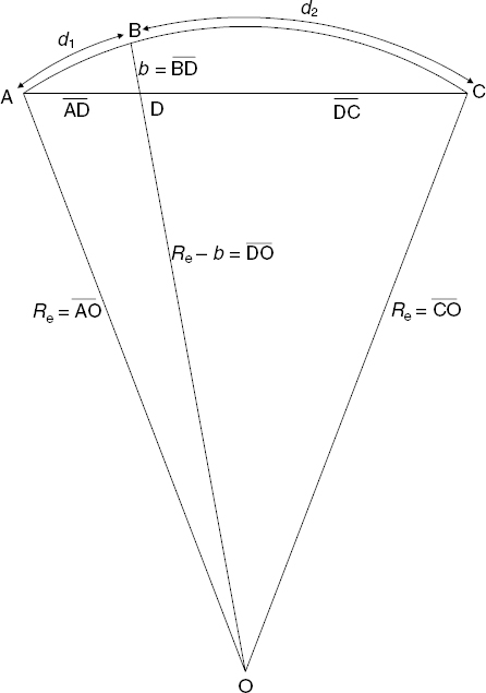
FIGURE 7.7 Calculation of Earth “bulge.”

Using this approach, the “bulging” of the Earth, that is, the vertical displacement of the spherical surface along the path, can be calculated by means of Figure 7.7. In this figure, ABC is a sector of the effective Earth surface with effective radius κa = R_e and center at O. In practice, the distance AC is on the order of tens of kilometers while R_e is several thousands of kilometers; if drawn to scale, BD (drawn perpendicular to the arc ABC at B) would also be almost precisely perpendicular to the cord AC at D. The distance BD = b is the “bulging” to be calculated; the distance DO therefore is R_e − b.

From Figure 7.7, using a theorem that relates the lengths of subsections of intersecting chords in a circle,

where

gives

and

In the above equations, b, d₁, d₂, and a are all in the same units. It is convenient to use d₁, d₂, and a in km or miles, but b in meters or feet. Using km and m,

meters. The Earth radius is approximately 6370 km (or 3960 miles), giving

meters, with the distances in km. This is a convenient equation from which the Earth “bulging” is plotted; since d₂ = d − d₁, the Earth bulge is a quadratic fit to the Earth's curvature as a function of d₁. With miles and feet as units, the corresponding relationship is

feet.

7.5 MICROWAVE LINK DESIGN

Proper point-to-point link design is governed by three considerations: (i) to minimize cost, one would prefer to space the stations far apart; (ii) if they are too far apart, the intervening Earth “bulge” will intercept the beam for some atmospheric conditions; (iii) if the intervening terrain is smooth, it will have a reflection coefficient of nearly −1. In that case, for certain antenna heights (which depend on the value of κ) the direct and ground-reflected signal will add out of phase and produce deep fades or signal loss. The aim of microwave link design is to assure proper path clearance and avoid destructive interference due to reflections; this requires consideration of the range of refractive conditions (i.e., κ values) that may occur at a specific location.

Consider two antennas within the line of sight as shown in Figure 7.8, with one antenna height (at the right-hand side B) variable. This figure represents a 30 km path. The arc near the bottom represents a convenient datum or reference height (such as 150 m AMSL (above mean sea level)) of the effective spherical surface of the Earth and is constructed by the use of equation (7.48). The terrain elevation above this level, obtained from maps or by measurement, is plotted to the same scale above the arc (i.e., added to the arc) to give the terrain profile. One end of the path appears at the left edge and the other at the right edge of the plot. At each edge a vertical scale, drawn to the same scale as the datum circle and terrain elevations, indicates possible antenna heights above the terrain.

FIGURE 7.8 Sample path profile.

When both antennas are 30 m above their respective terrains (path EF), the path is obstructed and transmission will be poor. If the antenna at B is raised from 30 m (F) to 60 m (G), the path appears to clear the obstacle. However, we should not expect a completely abrupt transition from the “obstructed” to the “clear” path condition. A quantitative understanding of this transition is needed.

We also note that as the antenna is raised, reflections become possible. If the arc CD represents a lake, the reflection EHG is highly likely (it should be noted that reflections often come from places that are not always obvious from the path profile plot because roads, large flat roofs, ballparks, flat pastures, etc. may not be apparent on these scales).

As discussed previously, a plot of the received signal power as one antenna height is varied, all other system parameters remaining fixed, is known as a height-gain curve. For the simple case of Figure 7.8 (one obstruction, one reflection point), the received signal strength relative to the strength that would be received in free space (without the surface below) might look as shown in Figure 7.9. This figure is similar to that observed for the planar Earth case (Figure 7.2) at higher receiver heights but is different at lower receiver heights due to the influence of obstructions caused by the terrain profile. On paths allowing more than one reflection, the height-gain curve is more complicated; nevertheless, the point A, where the field first reaches its free-space (Friis transmission formula) value, can often be identified with the obstruction, while minima such as B or C can be used to identify reflection points.

FIGURE 7.9 Sample plot of received power relative to free space versus receiver height: one obstruction, one reflection point.

7.5.1 Distance to the Radio Horizon

The “radio horizon” is the maximum distance by which a transmitter and receiver can be separated (Figure 7.10) and still remain within the radio line of sight, that is, the line of sight when refraction effects are included [1]. The modifier “radio” is often omitted below and in the literature. These concepts are applicable only in the VHF and higher frequency bands where groundwave and ionospheric effects are negligible.

A straight line ray between a transmitter at height h₁ and a receiver at height h₂ for path length d can be written as

FIGURE 7.10 Applicable geometry for determining the maximum radio line-of-sight distance for level terrain.

where d₁ is the distance along the Earth's surface from the transmitter. The Earth bulge is

Equating these two expressions determines the points of intersection (i.e., d₁ values) between the direct ray and the Earth bulge:

or

This equation is quadratic in d₁; the two roots of this quadratic will be imaginary when the path clears the bulge (no real intersection points) and real otherwise. When the path intersects the bulge in a single point, the quadratic has a double root at the intersection point. This is the situation that determines the radio horizon.

Applying the quadratic formula to equation (7.53) yields

To obtain a double root, the term inside the square root must be zero:

which is the quadratic equation to determine d = d_max, the maximum distance of the line of sight. Applying the quadratic formula a second time and finding the largest resulting root yields

which is the maximum distance by which antennas at heights h₁ and h₂ can be separated while remaining within each other's radio horizon. This does not necessarily imply that the link between the two will be effective! An adequate path clearance and freedom from destructive reflections are required, as will be discussed later in the Chapter. Note that d_max depends on the Earth radius multiplier, with smaller values of κ (which cause a larger Earth bulge) reducing the line-of-sight distance.

The distance to the radio horizon for a transmitter at height h₁ is obtained by setting h₂ to zero:

Using units of meters for h₁ and kilometers for d_horizon, as well as κ = 4/3, produces

Using miles and feet, we have

Thus, for example, a transmitter or receiver on an aircraft at 30,000 ft should see the radio horizon at a distance of approximately 245 miles. These results of course assume that the local terrain is sufficiently flat that only the curvature of the Earth need be considered.

7.5.2 Height-Gain Curves in the Obstructed Region

Obstruction by actual terrain may occur even for transmitters and receivers that would be within the radio line of sight if there were no obstructing obstacles. Since no simple mathematical solution is available for the diffraction of a radio wave by an arbitrary obstacle, our understanding of the effect of obstructions is derived from the solution of two canonical problems.

The first of these is the diffraction of an electromagnetic wave around a smooth conducting sphere. The geometry is shown in Figure 7.11 and the solution in Figure 7.12, curve A. Since no universal solution exists for spherical diffraction in the obstructed region, this curve was computed using the method of Chapter 9 for a 146 MHz transmitter at height 94 m and a receiver at distance 80 km whose height is varied to produce the curve illustrated. The path clearance is shown in Figure 7.11 by arrows; it is considered positive when the straight line (as represented on an equivalent Earth radius profile!) path clears the obstruction (Figure 7.11a), negative otherwise (Figure 7.11b). Although in real life h is perpendicular to the Earth surface, it appears vertical in the figure because of the very different scales in the vertical and horizontal dimensions.

FIGURE 7.11 Calculation of path clearance.

FIGURE 7.12 Received power relative to free space versus normalized path clearance: PEC sphere (146 MHz, 80 km path, 94 m transmitter height, varying receiver height), knife edge, and reduced reflection coefficient interference.

The horizontal axis of Figure 7.12 is expressed in terms of the ratio of the clearance h to the radius F₁ of the first Fresnel zone. In the unobstructed region h is measured, as usual, from the point where the reflection occurs. It can be shown that, for a smooth sphere, this point corresponds to the minimum value of h'/F₁ along each path, where h' is the distance from the path to the surface, perpendicular to the surface. This property was used in calculating Figure 7.12. In Figure 7.12 the abscissa is labeled in h/F1 (dimensionless) units, and the ordinate is the (also dimensionless) ratio of the actual field strength, , to what it would be in free space, .

Appreciable signal is present even when the path has negative clearance (e.g., EF in Figure 7.11). After the clearance becomes positive, the signal increases rapidly and attains the free-space value at h ≈ 0.6F₁, that is, when the path is cleared by approximately 0.6 times the radius of the first Fresnel zone at the location of the obstacle. Beyond this point, the curve behaves as we would expect from reflection theory. At h = F₁, the reflected ray reinforces the direct ray, causing a field strength , or 6 dB. At , the reflected ray cancels the direct ray, at , it reinforces, and so on.

The horizontal axis units in Figure 7.12 were chosen because it is found in many diffraction problems that the solution is “universal” in that it depends on the minimum value of h/F₁ encountered on the path and not independently on factors such as the path distance, antenna heights, and so on. For diffraction by a spherical surface, this is approximately true only for paths that clear the obstruction by 0.6 F₁ or more.

The second canonical problem, first solved by Arnold Sommerfeld, is that of diffraction by an infinite half-plane of zero thickness, as shown in Figure 7.13. The path clearance h is taken as positive if the direct ray clears the obstructing screen as for AB and negative if it is obstructed as for path AC. Because of the zero thickness assumption, the problem is sometimes referred to as “diffraction by a knife edge” in the literature; it is valid whenever the obstacle thickness is a small fraction of a wavelength. The solution for the knife edge problem is shown as curve B in Figure 7.12.

FIGURE 7.13 Canonical knife edge diffraction problem.

It is a curious coincidence, evident from Figure 7.12, that both the smooth sphere diffracted and the knife edge diffracted fields attain their free-space value with increasing h first when h/F₁ ≈ 0.6. This is also consistent with the planar Earth approach, where it was found in equation (7.39) that h/F₁ ≈ 0.577 provides a free-space propagation level. It is even more astonishing that this relationship generally holds true for actual propagation paths, even when these do not resemble either canonical problem. These results provide a useful “rule of thumb”: paths can be considered nonobstructed only when all obstacles are cleared by approximately 0.6 times the first Fresnel zone radius at the obstacle locations.

For obstructed paths, a variety of models have been described in the literature to predict the path loss; some models, such as in ITU-R Recommendation P.526-10 [2], also attempt to include the influence of multiple obstacles along the path. ITU-R Recommendation P.526-10 also provides an approximation to the knife edge curve in Figure 7.12 as decibels, where at the knife edge location; this approximation holds for h/F₁ < 0.55. An approximation for diffraction by a spherical Earth is also provided. In addition, ITU-R Recommendation P. 530-12 [3] uses the formula −10 + 20h/F₁ decibels as a general approximation for the received power relative to free space for h/F₁ < −0.25. However, it has been found that a wide variability in path loss can occur depending on the specific nature of the terrain profile, so producing accurate quantitative predictions through simple analytical means is difficult. Numerical approaches can provide some improvements, as will be discussed later in the chapter. For the moment, we will limit ourselves to classifying whether paths are obstructed or not. The knife edge prediction is also often used as an indicator of the maximum received power that is likely to occur.

7.5.3 Height-Gain Curves in the Reflection Region

When all obstructions are cleared, some minor signal variations due to the diffraction may still exist, but these are usually of little significance (see Figure 7.12 curve B for h/F₁ > 0.6). Instead, path behavior when all obstructions are cleared by at least 0.6F₁ is governed by reflections if any are allowed by the terrain. We have previously discussed (Section 7.3.1) the fact that such effects can be modeled for a single reflection point using

for the received power relative to free space, where h/F₁ is to be taken at the reflection point. Referring to Figure 7.12, curve A was for diffraction by a smooth conducting sphere. When h/F₁ > 0.6, the path is no longer obstructed, and curve A is predicted well by equation (7.60) with Γ = −1. For a rough surface, smaller amplitudes of Γ are applicable; curve C shows the result for Γ = −0.5. As stated previously, it is difficult in general to predict potential reflection points along a path profile without extensive knowledge of the terrain properties that is sometimes not available. In some situations, an analysis of multiple height-gain curves can be utilized to determine the location of reflection points.

For antennas in the reflection region that are separated by an appreciable fraction (30% or more) of the maximum line-of-sight distance, a modified direct plus reflected wave formulation is available that includes the effects of Earth curvature [1]. Two primary effects are important in this modified formulation: the determination of the reflection point location on a smooth curved Earth and a modification of the reflection coefficient Γ to include a “spherical divergence factor” that models the spreading of the reflected wave's energy by the Earth's curvature. Equation (7.60) remains applicable once these factors are included. This approach assumes that the Earth is a smooth sphere along the path of interest, a situation that is encountered infrequently for overland paths.

7.6 PATH LOSS ANALYSIS EXAMPLES

When a microwave path is to be used heavily (thus justifying high capital investment) and requires high reliability, the path may be tested by erecting temporary antenna towers and obtaining numerous height-gain curves with smaller, and hence more easily handled, antennas than will be used in the final installation. From these, all obstructions and reflective regions are identified. The performance of the path is then calculated for various antenna configurations and κ values, and the final configuration is chosen to maximize reliability for the range of κ values to be expected in that location.

Given a terrain profile, it is possible to make a preliminary prediction of the minimum transmitter or receiver height required in order to avoid obstruction for specified refractive conditions. Figure 7.14 illustrates a 36 km terrain profile to be used in an illustration of this procedure. Consider a 600 MHz transmitter located at the left side of the profile, at a height of 20 m above the local terrain. To avoid obstruction, a line drawn from this transmitter to a receiver at the right side of the profile must clear all terrain points by the Earth bulge plus 60% of the first Fresnel zone radius. Figure 7.15 plots the original terrain profile (solid curve) as well as the terrain profile plus the Earth bulge (using κ = 4/3) and 0.6F₁ (dashed). The minimum receiver height for which a free-space propagation level is predicted can now be determined by finding a line from the transmitter that intersects the dashed curve in only a single location. The line illustrated shows that the required receiver height is around 200 m above the local terrain.

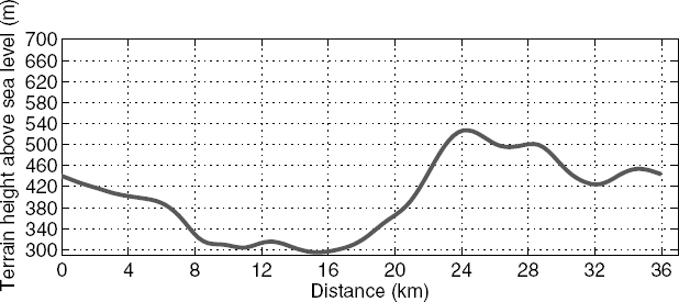
FIGURE 7.14 An example 36 km terrain profile to be used at 600 MHz with a transmitter at height 20 m.

If the location of a reflection point is known a priori, a similar process can be used to determine the location of maxima and minima in the height-gain curve. For a reflection point located at distance 24 km, the line tangent to the dotted curve in Figure 7.15 determines the receiver height near 280 m that causes destructive interference because the dotted curve is the terrain height plus the Earth bulge plus the second Fresnel zone radius.

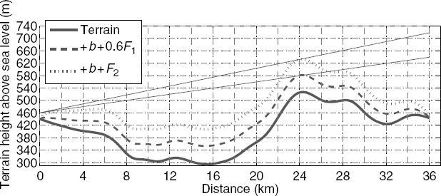
FIGURE 7.15 Determination of the minimum receiver height to achieve a nonobstructed path, and prediction of a receiver height experiencing destructive interference (assuming the hill at distance 24 km is the primary reflection point).

FIGURE 7.16 Paths giving free-space transmission for determination of obstructions.

For actual paths with hills and trees, the points of obstruction are not always obvious. The fact that the field reaches its free-space value, as antenna heights are increased, when the path passes 0.6F₁ above the obstruction point can often be used to identify the obstruction. In Figure 7.16, a group of propagation paths is shown that were found to give path loss equal to that of free space, that is, the path loss predicted by the Friis transmission formula. It is apparent that some paths are obstructed by the terrain at 16 km from the left end; however, paths that are low at the left end and high on the right end are obstructed at approximately 4 km distance. It would seem that the hill near 4 km is not high enough to cause an obstruction, but the particular cause of an obstruction or reflection may not be evident from the path profile, especially if it has been constructed from a topographic map instead of a careful survey. Buildings, forested areas, farm ponds, driveways, etc. are often not shown on such maps.

The location of the reflection points by similar means is also possible. At heights where the path is not obstructed, the curves will exhibit maxima due to odd Fresnel zone reflections and minima due to even Fresnel zone reflections (Figure 7.9, points B and C). The minima, being sharper, are better suited for locating reflection points. In practice, reflections may be possible over a region, in which case the precise reflection point will be determined by the path geometry, shifting to the left for paths inclined upward to the right, and vice versa. This makes the true crossings less distinct and more easily confused with any extraneous crossings. Also, the crossings multiply when several reflection regions exist.

A final example is presented in Figures 7.17–7.19 that compares a prediction of the free-space crossing height with measured data collected at 167 MHz by MIT Lincoln Laboratory researchers [4]. The 15.2 km terrain profile for this case is illustrated in Figure 7.17; the transmitter was located at 18.3 m above the local terrain at the left-hand side of the profile. Received power was measured as a function of receiver height at 15.2 km distance. Figure 7.17 also includes the terrain profile elevated by b + 0.6F₁ in order to determine receiver heights corresponding to the first free-space crossing. Lines are drawn to varying receiver heights until a receiver height is found that results in only a single intersection with the elevated terrain profile; the resulting ray and receiver height determination is shown in the figure. Note in this case that this ray almost intersects the elevated profile in two locations.

FIGURE 7.17 Beiseker N15 terrain profile for which propagation measurements at 167 MHz were performed by MIT Lincoln Laboratory [4]. Transmitter is located 18.3 m above local terrain at left of the profile. Dashed curve is terrain profile elevated by b + 0.6F₁ (κ = 4/3).

Figure 7.18 compares measured data with the predicted receiver height that obtains a free-space propagation level (marked by an “x”). For this example, the basic rule utilized appears to provide a good indication of the free-space crossing point, although the measured data cross the free-space power level at a slightly lower receiver height.

The height-gain curve in Figure 7.18 also shows significant multipath interference; the graphical methods we have learned can also be utilized to attempt to determine the location of the associated reflection point on the terrain. Given local minima in the measured height-gain curve at receiver heights 71.6 and 113 m, respectively, Figure 7.19 uses the graphical method to assess whether any intersections with the terrain + b + F₂ and the terrain + b + F₄ occur for these receiver heights at a common terrain location. It is found that a common intersection occurs near 13.2 km distance; the circles in Figure 7.18 mark the predicted minima locations in the height-gain curve, as well as predicted minima for clearance by F₆ and F₈. A reasonable agreement with the measured minima locations is obtained although some small differences remain. Note that the predicted received powers for these minima are assigned arbitrarily, as no knowledge of the local reflection coefficient is available.

FIGURE 7.18 Comparison of measured height-gain curve and graphical method predictions. Free-space crossing predicted using the rules of this chapter is shown, along with predictions of minima based on determination of two terrain reflection points. Results computed by a numerical method are also included.

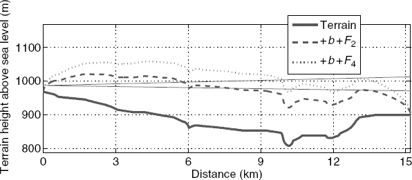
FIGURE 7.19 Determination of reflection point location, using knowledge of two receiver heights (71.6 and 113 m) observing minima in the height-gain curve of Figure 7.18. Common point of intersection is determined for rays to these receiver heights with the terrain elevated by b + F₂ and b + F₄, respectively.

It is interesting that even the first minimum here occurs at a power level that is around 1.5 dB larger than that received in free space, while a much stronger minimum occurs near receiver height 490 m. This suggests that more than one reflection may be present. An examination similar to that in Figure 7.19 was used to determine that the minimum near receiver height 490 m apparently results from an additional reflection point that is located at range 0.5 km from the transmitter. Figure 7.18 includes the predicted minimum location for this reflection point, marked with a diamond.

Figure 7.18 also includes the predictions of a numerical method that is found to provide a reasonable match to the measurements; such methods are discussed further in the next section. The path of Figure 7.17 was chosen here, in part, because both measurements and numerical results were available for comparison. It is, in some respects, unusual: the receiver was on a helicopter, enabling the continuous variation of receiver height to greater than 600 m, the results for only one transmitter height were examined, two distinguishable reflection points were present, and diffraction effects produced received power levels more than 6 dB greater than those in free space for some antenna heights.

7.7 NUMERICAL METHODS FOR PATH LOSS ANALYSIS

The ever increasing power of computers is now making numerical predictions of propagation over terrain possible. Instead of the simplified direct plus reflected and canonical diffraction analytical models studied earlier in the chapter, computers can be applied to solve Maxwell's equations with a specified irregular boundary surface (the terrain profile under investigation) and have been shown to yield reasonably accurate predictions when compared with measurements. Of course, the accuracy with which terrain and atmospheric refractivity profiles are known limits the numerical approach, but numerical methods can avoid many of the approximations in the solution of Maxwell's equations used by the analytical approaches, thereby obtaining a more accurate prediction.

Standard numerical techniques for electromagnetics, such as the method of moments, have been applied to propagation predictions, as in Ref. [4]. However, the large size of propagation problems on a wavelength scale often limits these studies because it is usually required in such methods to sample the electric field along the terrain profile at a rate of at least 10 points per electromagnetic wavelength. A more efficient numerical approach can be obtained by making a parabolic approximation to the wave equation that assumes that signals propagate nearly horizontally, which is reasonable for long-range propagation predictions between Earth stations. The parabolic equation (PE) method is also able to model variations in the atmospheric refractivity profile and can thus be used to study coupling effects between ducts and terrain irregularities. The reader is referred to the literature for additional information on such approaches; the “Advanced Refractive Effects Prediction System” (AREPS) produced by the Atmospheric Propagation Branch of the Space and Naval Warfare (SPAWAR) command (mentioned in Chapter 6) also includes a parabolic equation-based code.

The numerical results illustrated in Figure 7.18 were produced using a method of moments algorithm and required substantial computational time to be realized. Figure 7.20 compares these method of moments results (labeled “MOM”) with computations of a parabolic equation code (labeled “PE”); the curves are nearly indistinguishable in this example, indicating the generally high accuracy of the PE method for propagation problems. The terrain profiles used in these comparisons were obtained from a government mapping agency and contained terrain profile heights recorded at 30 m spacings. While the PE method utilized this profile directly, a linear interpolation between terrain profile points was used to obtain the much finer resolved surface required by the MOM approach. It was also assumed in both MOM and PE computations that the surface was perfectly conducting and that an effective Earth radius multiplier of κ = 4/3 was applicable.

FIGURE 7.20 Comparison of height-gain curves predicted by the method of moments and a parabolic equation code for the Beiseker N15 example of Figure 7.17.

7.8 CONCLUSION

The methods presented in this chapter have provided insight into the basic physical processes of multipath interference and diffraction by terrain. The path profile analysis rules we have utilized are intended for “point-to-point” applications for which terrain profiles are known, as opposed to “point-to-area” (i.e., broadcast) services or mobile systems. ITU-R Recommendation P.530-12 [3] provides additional information for these applications, including a discussion of diversity methods for overcoming destructive interference. The terrain profile information necessary for the application of these methods is available from several government agencies, including the U.S. Geological Survey; ITU-R Recommendation P.1058 [5] provides additional information on topographic data sets.

Our analyses have focused on a deterministic prediction of path loss properties given a specified value for κ; statistical information on κ can then be utilized to investigate statistics of the path analysis. Generally, it is the worst-case performance that is of interest. In addition, many mechanisms beyond reflections from terrain can cause multipath interference, including contributions from nearby objects (e.g., vehicles, buildings, etc.) Chapter 8 discusses example empirical path loss models for such situations and also introduces basic statistical fading models for predicting propagation losses.

REFERENCES

1. Fishback, William T. “Methods for calculating field strength with standard refraction,” in Kerr, Donald E. (ed.), Propagation of Short Radio Waves, McGraw-Hill, New York, 1951, pp. 112–140.

2. ITU-R Recommendation P. 526–10, “Propagation by diffraction,” International Telecommunication Union, 2007.

3. ITU-R Recommendation P. 530–12, “Propagation data and prediction methods required for the design of terrestrial line-of-sight systems,” International Telecommunication Union, 2007.

4. Johnson, J. T., R. T. Shin, J. Eidson, L. Tsang, and J. A. Kong, “A method of moments model for VHF propagation,” IEEE Trans. Antennas Propag., vol. 45, pp. 115-125, 1997.

5. ITU-R Recommendation P. 1058–2, “Digital topographic databases for propagation studies,” International Telecommunication Union, 1999.