4

ANTENNA AND NOISE CONCEPTS

4.1 INTRODUCTION

The function of a communication link is to transmit information from one location to another. If wireless radiowave propagation is to be used, the signal must be radiated from the transmitter site by a transmitting antenna. It then propagates toward the receiver site where a receiving antenna captures the signal and delivers it to a receiver system. As a result, it is difficult to specify the propagation process without reference to the antennas that transmit and receive the signal. The ability of a signal to be properly received at the receiver will depend not only on the power carried by the incoming electromagnetic wave, but also on the sensitivity of the receiver and the presence or absence of other (interfering) signals. Consideration of noise effects is therefore very important in the design of any communication system. The aim of this chapter is to develop the basic antenna concepts necessary for a discussion of propagation effects in wireless communication systems and to introduce standard methods for describing noise in communication systems so that prediction of signal-to-noise ratios (SNR) for realistic systems becomes feasible.

4.2 ANTENNA CONCEPTS

The field radiated from an antenna is always more complicated near the antenna than at a large distance from it. If one considers free-space propagation at distances sufficiently far from the transmitting antenna, the field appears to be a spherical wave emanating from a point (the antenna location). Under these conditions, the observation point is said to be in the far-field or Fraunhofer region of the transmitter antenna. Three conditions must be satisfied for this to be the case

where D is the largest dimension of the transmitting antenna, d the largest dimension of the receiving antenna, r the distance between the two, and λ is the wavelength of operation.¹ In communication systems, the receiving antenna is almost always in the far field of the transmitter antenna. Therefore, we will consider only far-field properties in this chapter.

4.3 BASIC PARAMETERS OF ANTENNAS

There are many ways of specifying antenna performance [1,2], and perhaps not all antenna experts would agree as to which ones are the most basic. For the purpose of this discussion, let us consider impedance, directionality, and efficiency as the most basic. Some other useful parameters that can be derived from these three will also be discussed.

The impedance of an antenna at a given frequency is defined to be the impedance it presents to a generator connected to its terminals. It can be measured by connecting the antenna to the source via an impedance bridge or a slotted line, just as other load impedances are measured. Simple in principle, such measurements can nevertheless be tricky in practice. Care must be taken that the environment, including the measurement apparatus, does not reflect energy, which the antenna has radiated, back into it. Therefore, such measurements must be performed outdoors or in an anechoic chamber; that is, one that has walls made of absorbing material. Another precaution is to make sure that the antenna is not in the field of any signal that it can receive, especially if the measurement requires obtaining a null. For example, when the impedance of a broadcasting antenna is measured with an impedance bridge, a good balance cannot be obtained when a signal from another station on the same channel is present.

The antenna impedance is, in general, composed of a resistive component (real part) and a reactive component (imaginary part),

The resistance indicates the time averaged power P delivered to the antenna when a sinusoidal current is applied to the terminals:

where is the peak current amplitude. Part of the input power is radiated by the antenna P_r, and part is dissipated as heat in the antenna structure (ohmic losses) P_l, so

Although the focus of the current discussion is on the antenna impedance, note that the time-averaged radiated power P_r can be obtained as an integral of the real part of the complex Poynting vector over a closed surface A surrounding the antenna

if the radiated fields and are known on the surface A.

In terms of P_l and P_r, the loss resistance of the antenna is defined as

and the radiation resistance as

Note that the factor 1/2 in equations (4.3) and (4.5) and the factors of 2 in equations (4.6) and (4.7) are a consequence of the use of peak as opposed to rms value phasors.

It is then found from equations (4.3) and (4.4) that

The radiation efficiency of an antenna at a given frequency is a second basic quantity. It is defined as the ratio of the total power radiated by the antenna to the total power delivered to its terminals:

From (4.4)–(4.8) follow the relations

The concept of radiation efficiency is simple, but its measurement is again by no means an easy matter. One method consists of measuring the radiated power density at a sufficient distance in all directions for which it is significant and integrating this to get the total radiated power P_r. The input power P is measured at the same time, and radiation efficiency is calculated from equation (4.9). In another approach, the antenna impedance is first measured with the antenna radiating into space. Next the antenna is surrounded at a sufficient distance with a conducting shell, and its impedance is remeasured. Assuming the antenna current is unaffected by the shell, and also assuming the losses in the shell are much smaller than those in the antenna, the losses will be the same for both measurements, and the resistive part of the impedance measured in the second case will be R_l while that measured in the first case is R_A. The radiation efficiency can then be computed from equation (4.10).

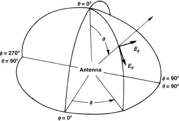
FIGURE 4.1 Antenna coordinate system.

A third basic property of an antenna system is its directional performance at a given frequency. To specify this, a spherical coordinate system with the antenna at its center can be employed, as shown in Figure 4.1. At the given frequency, the relative field strength of the θ component amplitude and phase in a given direction can be given by a phasor ; similarly, the relative φ component can be specified by a phasor . The total electric field at a distance R in the far field is then given by the complex vector function

where the term e^−jkR/R captures the range dependence of the field and describes a “spherical wave” behavior. This dependence on range is true in the far field of any antenna, with different antennas producing different and . Unlike plane waves, fields radiated from an antenna decrease in amplitude as the reciprocal of the distance from the antenna. However, for large R, small changes in R do not cause significant amplitude variations and the field can be approximated as a plane wave in many applications.

In practice, it is more usual to measure the “relative power patterns” P_θ(θ, φ) and P_φ(θ, φ) for θ and φ polarizations, respectively, expressed as

FIGURE 4.2 Directional pattern measurement.

where is an arbitrary normalization constant. Unless one of these power patterns is zero, this is not enough information to give the antenna response to arbitrary polarization. The missing information is the phase relationship between the and phasor functions in a given direction, which can be obtained by measuring the power pattern of a judiciously chosen third polarization.

Relative field strength and power patterns can be measured by rotating the test antenna while a signal is being transmitted between it and another sufficiently distant antenna, as shown in Figure 4.2. The transmission path must be long enough to ensure that, if the test antenna is used as a transmitter, the field produced by it will be represented with sufficient accuracy by a plane wave over the receiving antenna aperture. In practice, transmission may be in either direction; that is, the test antenna can equally well be at the receiving end. Sometimes it is not practical to have sufficiently long links to carry out such measurements. If a measurement is done using a shorter link, lenses or reflectors can sometimes be used to generate a planar wavefront at the receiver antenna location. Such antenna pattern measurement ranges are called compact ranges. Care must be taken to ensure that the measured signal from the transmitter antenna reaches the receiver antenna solely via the direct transmission path, with no significant reflections from the ground or other structures (such as supporting structures) reaching the receiver antenna. Obviously, rotating an antenna structure is practical only when the antenna is reasonably small. One way of overcoming this difficulty for large antennas (meant to operate at relatively low frequencies) is based on the concept that the antenna patterns depend not on the absolute size of the antenna, but instead on the size measured in wavelengths— in other words, on the electrical size of the antenna. Thus, it is possible to obtain the patterns by measuring a scale model of the desired antenna. For example, the antenna may be scaled down in size by a factor of 20, provided the wavelength is also scaled down by a factor of 20, that is, provided the frequency used for measuring the model is 20 times the frequency at which the full-scale antenna is intended to operate. It is assumed in such an approach that the dielectric properties of all the antenna materials do not vary significantly between the original and scaled frequencies.

In a typical measurement, the patterns will be only relative values, but in theoretical treatments, it is sometimes useful to normalize the patterns. A particularly convenient normalization is the directional gain of an antenna D(θ, φ), defined as the ratio of the power density radiated in the direction (θ, φ) to the power density at the same distance that would be radiated by an isotropic antenna² with the same polarization and radiation efficiency, and with the same input power. If a receiving system is available that is calibrated absolutely, the directional gain may be determined as

where the tilde denotes an absolute measurement (in W/m²) and R is the measurement distance. Alternatively, D(θ, φ) can be expressed from uncalibrated relative power measurements by

given the relative power patterns P_θ(θ, φ) and P_φ(θ, φ). It is then necessary to measure P_θ(θ, φ) and P_φ(θ, φ) for all directions (θ, φ) into which significant power is radiated. It is also commonplace to report the directional gain for only a given polarization. For example, for vertical polarization only the first term in the numerator of equations (4.14) or (4.15) would be used.

The gain of an antenna in a given direction is the product of directional gain and efficiency

By the use of equation (4.14), this can be shown to be equivalent to

which at a specified distance R determines the power density radiated in a given direction relative to the input power. This is a very important measure of antenna performance.

Some examples will illustrate these concepts. Consider a vertically polarized (θ polarized) isotropic antenna; for such an antenna, we should have P_θ = C₁ and P_φ = 0, where C₁ is some arbitrary constant. From equation (4.15), one then finds D(θ, φ) = 1, or 0 dB. Consider now a small dipole with uniform current distribution (Hertzian dipole). For such a dipole, the radiated power density is distributed in space according to P_θ = C₂ sin² θ, P_φ = 0, where C₂ is again an arbitrary constant (depending on the current strength and the distance) and θ is the polar angle measured from the dipole axis. Use of these P_θ and P_φ in equation (4.15) gives D(θ, φ) = 1.5 sin² θ.

The directivity of an antenna is defined to be the directional gain in the direction that maximizes it; that is, it is the maximum directional gain for a given antenna. It is typically denoted by D(without any arguments since it is a number). For the isotropic vertically polarized antenna, D = 1, or 0 dB; for the Hertzian dipole, D = 1.5, or 1.8 dB.

The gain of an antenna can also be specified as G without any argument. In this case, it refers to the gain G(θ, φ) in the direction (θ, φ) that maximizes it. For a 100% efficient vertically polarized isotropic antenna, equation (4.16) shows that G = 1, or 0 dB, while for a perfectly efficient Hertzian dipole, it shows G = 1.5, or 1.8 dB. This means that for a given input power and distance a Hertzian dipole produces 1.5 times the power density that would be produced by an isotropic antenna of the same efficiency in the direction of maximum gain. It should be apparent that gain is a very important measure of antenna performance.

4.3.1 Receiving Antennas

Our discussion so far has focused on the use of antennas as transmitters. It is also important to understand the reception of electromagnetic waves by antennas. It is possible to develop this subject through use of the “reciprocity theorem” of electromagnetics. However, a more direct approach is utilized here by considering the case of a short wire receiving antenna and generalizing the equations that result to other antenna types.

In the early days of radio, the prototypical transmitting antenna was a metal mast fed against the Earth, which was sometimes made more conductive by a buried screen of wires. A wire screen was sometimes also inserted at the top of the mast (called the “top hat”) to give the vertical current along the mast (which was the main contributor to the radiation) a place to flow. The current would enter the top hat, gradually dropping to zero at its outer edges. In this fashion, the vertical current amplitude was relatively constant over the length of the vertical mast. A sketch of such an antenna is shown in Figure 4.3a. A uniform current dipole that would radiate (by the image theorem) an identical field in the region above ground is shown in Figure 4.3b. At the receiver in the plane θ = 90°, the field of such a dipole is given by

where h is the total length of the dipole and η₀ is the free-space impedance (≈ 377 Ω). The expression for the field of any arbitrary antenna in the far field (equation (4.11)) shows that this can be written in a form that is an analog to equation (4.18) as

where I is the input current. The complex vector defined by this equation is a characteristic property of the antenna and is called the complex vector effective height. For antennas radiating only one polarization, its magnitude is sometimes simply called the effective height. The term effective length and symbol are used interchangeably with effective height and , respectively.

FIGURE 4.3 Origin of the “effective length” concept. (a) Typical low-frequency transmitting antenna. (b) Equivalent uniform current dipole.

The performance of a receiving antenna is fully characterized by its transmitting properties provided it does not include nonreciprocal devices or materials, which are unusual. Assuming that an incoming field is arriving from the direction (θ, φ), the power delivered by an antenna to a load Z_R connected to its terminals is given by the equivalent circuit as shown in Figure 4.4, where the Thevenin voltage is given by

where Z_A represents the antenna impedance (i.e., the same impedance that the antenna would have as a transmitting antenna) and Z_R is the receiver input impedance. Thus, for an antenna that is responsive to only the same single polarization, for example, a dipole, the Thevenin generator voltage in Figure 4.4 is simply given by

FIGURE 4.4 Equivalent circuit model for receiving antenna.

Since we use peak value phasors, the time-averaged power delivered to the receiver can be calculated from the equivalent circuit in Figure 4.4 as

where the θ and φ arguments have been omitted for brevity.

At frequencies below about 30 MHz, long straight wires are commonly used as antennas, and h_e, the magnitude of , turns out to be on the order of the physical length of the wire, but always somewhat less. This interpretation in terms of an effective length is quite general, but it is of course physically more appealing for straight wires. As a result, it is used mostly in the frequency ranges where straight wires happen to be useful antennas.

At microwaves, straight wires are seldom used, and it is much more common to employ, for example, horns or reflector antennas. Such antennas are characterized by an aperture (a characteristic area) rather than a length. For this reason, it is useful to obtain a relationship between the effective height and antenna parameters, such as gain, in the microwave range.

To begin the process of deriving such a relationship, it is useful to express as the product of a magnitude (real and positive) factor and a complex unit vector

where the magnitude factor is defined as

and the unit vector by

Similarly, the electric field vector can be written as

From equation (4.19), we can obtain the far-field power density expression from the peak value phasor field for any antenna as

This flux density can also be calculated from input considerations. The power input to the antenna is given by equation (4.3), so that for an isotropic antenna the flux density at distance r would be . Hence, for an arbitrary antenna we have from (4.14)

Equating equations (4.28) and (4.27) yields

which is the relationship we are looking for. Its use, together with equations (4.24) and (4.26), in equation (4.22) results in

The first factor in the above expression is the flux density S of the wave arriving from direction (θ, φ). The second factor has the dimension of area. The remaining three factors are dimensionless. In particular, the factor involving the unit vectors depends only on the antenna polarization and the polarization of the arriving wave and represents the polarization mismatch factor, typically denoted as p. The polarization mismatch factor has a maximum value of unity when the antenna polarization is ideal for the impinging wave. It is not difficult to show (with proper attention to the relationship of the coordinate systems of the transmitting and receiving antennas) that the optimum receiving antenna polarization is the same as the transmitting antenna polarization. Thus a wave launched with a right circular polarized antenna should be received with a right circular polarized antenna. The last factor is the impedance mismatch factor, denoted as q. The impedance mismatch factor has a maximum value of unity when . Equation (4.30) can therefore be written in the form

where the maximum effective aperture or area A_em is given by

with polarization mismatch factor

and impedance mismatch factor

The product of the last four factors in equations (4.30) and (4.31) is sometimes called the receiving aperture or area. Since the maximum of the last three factors is unity, the receiving aperture cannot exceed A_em and hence the nomenclature maximum effective aperture for that quantity. The effective aperture A_e is the product

For aperture-type antennas, the maximum effective aperture is usually close to, but somewhat less than, the physical area projected on a plane perpendicular to the propagation direction. This is generally not true for other antenna types. For example, a half-wavelength (0.5λ) dipole has a directivity of 1.64, which corresponds to a maximum effective aperture of 0.13λ². Thus, it effectively absorbs power as though it had a width of (0.13λ²)/(0.5λ) or 0.26λ, even though the diameter of such a dipole is usually very much smaller.

The concepts of effective length, gain, and effective aperture will be especially useful in connecting propagation with the transmitter at one end and the receiver at the other, thus allowing propagation calculations to be used as one step in the overall process of estimating the performance of communication or radar systems in which wireless propagation is involved. Only an introductory treatment of antennas and their properties has been provided here; the reader is referred to many books on antennas, for example, references [1, 2], for additional information.

4.4 NOISE CONSIDERATIONS

The performance of systems that deal with information, such as communication links and radars, depends greatly on the signal-to-noise-ratio (SNR) at the receiver. Part of the noise originates from within the receiver system itself; this type of noise is called internal noise. All other noise (e.g., undesired interfering signals and static) is called external noise.

4.4.1 Internal Noise

All electronic devices produce small randomly varying electrical signals due to the thermal motions associated with their constituent atoms. These fluctuations, although they are small, are important when the signal is small. The receiver also receives noise generated by the antenna resistance R_A or by the internal resistance of a signal generator connected to its input. The standard equation for the thermal noise power emitted from a resistor at absolute temperature T in bandwidth B (in Hz) is given by

where N_i is the emitted noise power and k_B = 1.38 × 10⁻²³ J/K is Boltzmann's constant. Although equation (4.36) holds for a resistor at absolute temperature T, it is often used to define an equivalent “noise temperature” for any source of noise power N_i by T = N_i/(k_BB). Thus the noise input from the antenna or signal source can be specified either as a noise power or as an equivalent noise temperature.

A receiver contains many electronic parts, and the use of (4.36) for each component is not feasible. Instead, a more easily measured quantity denoted as the noise factor is used generally to quantify amplifier performance with regard to noise. The noise factor (also known as the noise figure) of an amplifier is defined by

where S_i and N_i are the available signal and noise input powers applied at the amplifier input and S₀ and N₀ are the available signal and noise output powers that result. The “available” implies that both the source and the load of the receiver or amplifier are terminated in a matched load, and this will be assumed throughout the remainder of this section. Standard noise factor measurements are made at a temperature T₀ = 290K, corresponding to N_i = k_BT₀B (W). This temperature is chosen as an approximation to the usual operating conditions; the standard noise factor would not be appropriate for a cryogenic receiver. Note that S_i/N_i is not the actual input SNR if there is a mismatch at the receiver input. Also, note that the noise figure is ≥ 1, with unity representing an idealized receiver that adds no noise, because the output SNR cannot exceed the input SNR.

If an “available power gain” is defined as

then the noise figure can be written as

The output noise consists of the amplified input noise plus some additional noise N_N added by the receiver components, therefore

It is sometimes useful to refer the additional noise to the input, resulting in a quantity known as the excess noise N_e ≡ N_N/G_A. Equation (4.40) then becomes

Recalling N_i = k_BT₀B under standard conditions and rearranging (4.41) gives

where F is the standard noise factor and N_e is the excess noise contributed by the receiver when referred to the input. In receivers containing several amplifier stages, most of the internal noise comes from the first stage, since noise generated by this stage will be amplified by the full gain of the receiver, while noise generated by later stages is subject to less amplification. Thus, a low-noise amplifier is most often found as the first stage in a receiving system.

In microwave systems both the input and the output of amplifiers are usually matched, so that G = G_A (the true power gain) and S₀/N₀ is the true SNR at the output. Then

which is applicable when the input noise N_i is the standard k_BT₀B.

An equivalent circuit that models noise generated by the receiver or amplifier as being applied at the input, according to equation (4.43), is shown in Figure 4.5. In this figure N_e represents the excess noise, generated within the receiver or amplifier and referred to the input, while N_i represents the noise contribution from the signal source.

One method of measuring internal receiver noise directly is to orient a receiving antenna so that very low input signal and noise power are received (e.g., by directing the antenna toward a quiet part of the sky if this is possible and the antenna has sufficient directivity). The resulting noise power at the output comes from the receiver and the antenna. The antenna loss noise can be neglected if the antenna is highly efficient; then the output noise can be divided by the gain to calculate the excess noise referred to the input. From Figure 4.5, we have

FIGURE 4.5 Equivalent circuit for noise contributions.

which allows the calculation of signal-to-noise ratio at the output of a receiver given the input signal (S_i) and noise (N_i) powers, as well as the standard receiver noise figure F.

4.4.2 External Noise

A somewhat loose distinction needs to be made here between external noise and interference. In a sense, they are alike in being unwanted signals that have deleterious effects on system performance. If the unwanted signal is man-made and has characteristics not too unlike that of the desired signal, it is likely to be termed interference; otherwise, it is termed noise. Here, our focus is on noise received by the antenna from external sources.

The fundamental measure of external noise is the noise brightness of the source, B_s(f, Ω), measured in watts per square meter per steradian per hertz. The direction at which the source is seen in the receiving coordinate system will be denoted by Ω, and dΩ is the increment of solid angle, dΩ = sin θ dθ dφ. The noise brightness is a property of the source and does not depend on the distance from which it is viewed.

The analogy to vision may be useful here.³ Concentrate on a single pixel, that is, the smallest solid picture element that can be resolved. The radiant flux density responsible for that pixel seems to come from a single direction, but actually it corresponds to the integration of brightness over the acceptance angle of the eye. A change in the distance between source and receiver does not change the observed brightness, but it does change the received flux density because the angle subtended by the source changes with distance.

Similarly, the received external noise power at the output of a receiver is given by an integration over the view angle and frequency:

In this equation, H denotes the (unitless) receiver system transfer function and T_p the physical temperature of the antenna in degrees Kelvin. As before, A_em is the maximum effective aperture of the antenna, q is the antenna impedance mismatch factor, p is the polarization mismatch factor, υ is the radiation efficiency of the antenna, and k_B is Boltzmann's constant. The term involving T_p gives the noise power due to antenna losses. It should be omitted if the antenna noise is included in the internal noise N_i. Its contribution is often small for well-designed antennas.

When the relationships between the antenna parameters are used,

the result is

Often, all the quantities in equation (4.47), with the exception of H(f), do not vary appreciably over the receiver passband. The integration with respect to frequency can then be replaced with multiplication by a noise bandwidth B, defined as

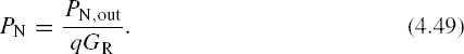
where G_R is the nominal receiver gain, typically taken as the average value of |H(f)|² over the passband. Also, it is usual to specify the maximum available noise as referred to the input,

The result is

This simplification will be used hereafter, with the understanding that it is not applicable when the noise brightness of the source has a substantial frequency dependence within the receiver passband. The reader should be able to derive the corresponding expressions including frequency integration without difficulty.

4.4.2.1 Source Brightness Temperatures Often the source brightness is specified, not directly, but in terms of an equivalent brightness temperature, the temperature that a blackbody would need to have in order to radiate with the same brightness as the actual source in the antenna polarization. A “blackbody” is an idealized source that perfectly absorbs all incident radiation and reemits this radiation as thermal noise. For blackbody radiation, the brightness at frequency f is related to the physical temperature T by Planck's law

where h is Planck's constant. For reasonably warm sources, the exponent in this equation is small and the first two terms of a Maclaurin series expansion of the exponential suffice. Also, for blackbody radiation the polarization is random so that only half of the radiation is emitted with the antenna polarization, and therefore p = 1/2. When these considerations are used, the result is

which gives

For blackbody radiation, the “brightness temperature” is the physical temperature of the source. The concept is extended to other radiation sources by defining a brightness temperature by equation (4.52). The maximum noise power available at the antenna terminals, P_N, may also be represented as an equivalent antenna temperature T_A

or as an equivalent standard receiver noise factor F_ext

where T₀ = 290K is the standard reference temperature. Thus, equation (4.53) can be written as

When the source brightness is constant over the entire antenna beam, T_B in equation (4.56) can be taken out of the integral, and the with use of

it follows that

In this case, the antenna noise temperature is the weighted average of the source brightness temperature and the physical antenna temperature. It should be remembered that the three temperatures in this equation come from very different concepts. T_p is the physical temperature of the antenna. T_B is the brightness temperature of the source; for blackbody radiation, it relates directly to Planck's law, and for other radiation indirectly so. T_A is the temperature at which a resistor matching the receiver input would give the same noise output as that actually obtained. Three distinct concepts of temperature are involved here!

If the source subtends such a small angle at the receiver that it cannot be resolved, G(Ω) and p(Ω) can be held constant in the integration with respect to Ω in equation (4.50). The integration of brightness over view angle gives the flux density arriving from that range of view angles; thus, for an unresolved source in the direction Ω₀

FIGURE 4.6 Typical values for equivalent external noise figure (F_a) and antenna temperature, t_a, from 0.1 Hz to 10 kHz. (Source: ITU-R Recommendation P.372-9 [3], used with permission.)

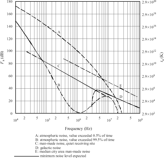
FIGURE 4.7 Typical values for equivalent external noise figure (F_a) and antenna temperature, t_a, from 10 kHz to 100 MHz. (Source: ITU-R Recommendation P.372-9 [3], used with permission.)

where S_N is the noise flux density (W/m²) arriving from the source. The result of using this equality in equation (4.50) is

An rms noise field strength E_N can be defined by

where η₀ is the free-space impedance, resulting in

with P_N the maximum available external noise power at the input when the antenna and receiver are impedance matched (q = 1). Comparing this result with equation (4.30) shows that the system treats noise that arrives as a plane wave from a single direction just as a signal smeared over the receiver bandwidth. This is what might well be expected!

FIGURE 4.8 Typical values for equivalent external noise figure (F_a) and antenna temperature, t_a, from 100 MHz to 100 GHz. (Source: ITU-R Recommendation P.372-9 [3], used with permission.)

Figures 4.6–4.8 plot typical external noise levels from 0.1 Hz to 10 kHz, 10 kHz to 100 MHz, and 100 MHz to 100 GHz, respectively, versus frequency. These plots are in terms of an “equivalent external noise figure” F_a = 10 log₁₀ (T_A/T₀) (left-hand side axis labels) and also in terms of T_A (right-hand side axis labels). For lower frequencies, the atmospheric noise in Figure 4.6, sometimes also called “atmosferics” or simply “sferics,” is the noise radiated by lightning, which may be propagated ionospherically over long distances. At a single location, especially in the temperate climate zone, lightning may seem to be a moderately rare phenomenon; on a worldwide basis, however, lightning occurs almost continuously. The static heard between stations on the AM broadcast band in the United States (540–1700 kHz) is due to sferics. Sferics are usually the dominant noise source below about 10 MHz. Figures 4.6–4.8 illustrate the relative importance of various noise sources as a function of frequency and show a transition from lightning, galactic, and man-made noise at lower frequencies to “sky” and “solar” contributions at higher frequencies.

FIGURE 4.9 Typical values for the atmospheric brightness temperature at various elevation angles, 1–350 GHz. (Source: ITU-R Recommendation P.372-9 [3], used with permission.)

Figure 4.9 shows the sky brightness temperature due to emission from the gases that absorb in the microwave region, namely, water vapor and oxygen. We will see in Chapter 5 that the frequency bands of high naturally emitted thermal noise correspond to frequency bands of high absorption by atmospheric gases. The multiple curves in the figure are for various elevation angles at which the sky is viewed. These curves depend on meteorological factors, including vertical profiles of atmospheric temperature and water vapor, as will be discussed for Chapter 5 with regard to the total attenuation through the atmosphere. The fact that the radio noise emitted by the atmosphere depends on meteorology enables “remote sensing” of atmospheric properties by measuring emitted noise; sensors of this type are called “microwave radiometers.”

Additional information on external noise values and their variations with geographic location and season is provided in ITU-R Recommendation P.372 [3].

REFERENCES

1. Kraus, J. D., and R. J. Marhefka, Antennas for All Applications, third edition, McGraw-Hill, 2001.

2. Stutzman W. L., and G. A. Thiele, Antenna Theory and Design, second edition, Wiley, 1997.

3. ITU-R Recommendation P.372-9, “Radio noise,” International Telecommunication Union, 2007.