3

PLANE WAVES

3.1 INTRODUCTION

Maxwell's equations (equations (2.1)–(2.4)) are very elegant and concise, but elegance should not be confused with simplicity. There is nothing simple about four coupled vector partial differential equations! Nor should we expect simplicity since these equations are to describe all propagation modes in all possible media. The complexity of the mathematics reflects the complexity of the physical phenomena it serves to describe.

Since the general case is too complex to solve analytically, one is forced to make simplifying assumptions to find some simpler analytical solutions. Plane waves turn out to be the simplest solutions of Maxwell's equations [1–4]. Despite their analytical simplicity, plane waves find physical applications in a wide range of scenarios. More complex solutions are generally required to describe electromagnetic fields in the vicinity of sources, or close to material discontinuities and/or inhomogeneities in the propagation medium. Far from such regions, plane waves are in general a very good description for the local electromagnetic field behavior. Furthermore, in more complex cases, the total solution can often be represented as the superposition of a set of plane waves with varying amplitudes and propagation directions, in a manner analogous to a Fourier (or spectral) decomposition. Therefore, plane wave solutions are worthy of special attention.

3.2 D'ALEMBERT'S SOLUTION

To simplify the derivations below, we consider a charge-free and nonconducting medium of the simplest kind discussed in Chapter 2, that is, isotropic, linear, dispersionless, homogeneous, and time invariant. Maxwell's equations then reduce to

If one takes the curl of both sides of the first equation, makes use of the fact that ∈ is a constant for a “simplest” material, that time and space are independent variables so that order of differentiation is immaterial, and finally substitutes from equation (3.2), one gets

Noting that μ is constant (for the same reasons as those applied to ∈), there results

Similarly, if one takes the curl of equation (3.2) and uses equation (3.1) as the auxiliary relation, one obtains

Equations (3.6) and (3.7) are known as the vector Helmholtz (or wave) equations. Their advantage over Maxwell's equations is that their independent variables appear uncoupled, equation (3.7) involving only the electric field and equation (3.6) only the magnetic field. By use of the vector identity

and equations (3.3) and (3.4), one obtains the vector wave equations

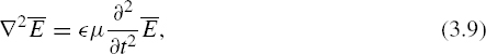
where the symbol ∇² operating on a vector denotes the Laplacian operator applied to each Cartesian component; for example, equation (3.9) stands for

Again, we must distinguish between elegance and simplicity: equation (3.9) is elegantly concise, but its equivalent equation (3.11) shows that it is far from simple. Nor should this surprise us. We have assumed the medium to be a simple one locally, but at any distance there might be obstacles or inhomogeneities, and nothing whatever has been said about sources, so that the field may be quite a complicated one.

To simplify equation (3.11) so that a solution may be obtained, let us assume that all derivatives with respect to y and z vanish. Physically, this is equivalent to requiring the problem to be invariant along those directions. Taking the three components of equation (3.11) separately, we now have three relatively simple equations

It can be shown now that equation (3.12) does not lead to a useful solution. Equation (3.3) and the assumption we have made that all derivatives with respect to y and z vanish require

Using the fact that derivatives with respect to y and z vanish in equation (3.1) results in

and hence E_x is constant in time (a static or DC field). Since information is carried only by signal variations, this field plays no part in the information transmission process. Therefore, we will neglect it, while keeping in mind that static fields may always exist superimposed on the signals we are treating.

Equations (3.13) and (3.14) are of the form

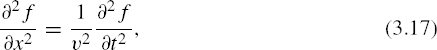
which was first shown by d'Alembert to admit solutions of the form

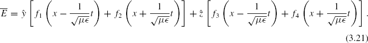
where f₁ and f₂ are arbitrary twice-differentiable functions. Accordingly, we find

Here, the f_n, n = 1, 2, 3, 4 are arbitrary twice-differentiable functions. The time variation of the source will determine the particular functions that are appropriate to a given problem. In vector form,

Taking the curl of both sides of this equation and recalling that only x derivatives are nonvanishing, we get

where the prime denotes a derivative with respect to the argument. Now we can apply equation (3.2) to get

Noting that

and that the constant C represents a static or DC field, which can be neglected as before, we have

with the argument of each f_n in (3.27) the same as in (3.21).

3.3 PURE TRAVELING WAVES

The arguments of the f_n functions appearing in equations (3.19)–(3.25) are of two kinds. The functions f₁ and f₃ always appear with the argument , while f₂ and f₄ always appear with argument . Let us assume for the moment that f₂ and f₄ are zero and that f₁ at t = 0 has the space dependence as shown in Figure 3.1a. From this we infer that f₁(u), where , has the form of Figure 3.1b. Hence, we can find the space dependence of f₁ at any other time; the dependence at time is shown in Figure 3.1c. We see that the form of the wave has not changed at all, being determined entirely by the shape of f₁. What has happened is that between t = 0 and the wave has traveled 2 units in the x direction. Thus, f₁ represents a wave traveling, without change of form or amplitude, in the x direction. Its velocity, called the wave velocity, is . The same is true of f₃. Any wave for which f₂ = 0 = f₄ is a pure traveling wave in the +x direction. Similarly, f₂ and f₄, which have the argument , can be shown to represent a wave traveling without change of amplitude or shape in the −x direction; thus, any wave for which f₁ = f₃ = 0 represents a pure traveling wave in the −x direction. From equations (3.21) and (3.25), it follows that for either set of traveling waves the relations

FIGURE 3.1 (a) Space dependence of f₁ at t = 0. (b) Dependence of f₁ on u as found from (a). (c) Space dependence of f₁ at t = 2/υ, as found from (b).

are obeyed, where the wave impedance η (also known as the characteristic impedance or the intrinsic impedance of the medium) is given by

FIGURE 3.2 Space relationship for TEM wave vectors; denotes the propagation direction.

and is the unit vector in the propagation direction; that is, for f₁ and f₃, and for f₂ and f₄. Equations (3.26) and (3.27) are by far the easiest way for finding one of the fields (electric or magnetic) of a pure traveling wave when the other is known, and they will be used so often that it is worthwhile to know them by rote. They show that , , and are three mutually perpendicular vectors. Such waves are called transverse electromagnetic (TEM) waves because both the electric and magnetic vectors are transverse to the direction of propagation, as shown in Figure 3.2. They are also referred to as plane waves because the and fields do not vary in any plane perpendicular to the direction of propagation.

3.4 INFORMATION TRANSMISSION

D'Alembert's solution is of fundamental importance to the concept of transmitting information by electromagnetic waves. It guarantees that, to the extent that a medium satisfies the approximation of a nonconducting “simplest” medium, a plane wave propagating in this medium with a waveform impressed upon it will emerge at the receiver unaltered in shape, with the information intact. The process of shaping the waveform at the transmitter according to the information to be transmitted is called modulation and that of recovering the information from the wave at the receiver is called demodulation or detection.

The conditions that were stipulated for the medium, that it be nonconducting and otherwise simple, were necessary, as can be shown by substituting equations (3.21) and (3.25) into Maxwell's equations: when these conditions are not satisfied it is found that they are no longer solutions. Thus, departure from the ideal properties causes the signal to be distorted during propagation; the greater the departure from the ideal and the longer the path, the greater the distortion. The concept of bandwidth comes in handy here. In general, media that are nearly ideal have wide bandwidth, while those that depart greatly from the “simplest” case have narrow bandwidths. The troposphere departs from an ideal medium primarily by having only slight inhomogeneities; its bandwidth for most propagation processes is many megahertz. The ionosphere is a plasma that has a very strongly dispersive as well as anisotropic and conductive character; its bandwidth for most propagation modes is on the order of only a fraction of a kilohertz to a few kilohertz.

In principle, it is not necessary for a medium to be nondistorting to propagate information satisfactorily, as long as the signal information can be reconstructed at the receiver. In practice, of course, such reconstruction can be difficult if the distortion is strong. For certain digital signals, distortion in the medium can cause intersymbol interference (ISI), necessitating the use of channel equalizers, for example. For digital signal transmission, the reliability of data transmission can be improved by adding redundant data in the signal by means of forward error correcting codes. One complicating factor is that for natural media such as the troposphere and ionosphere, the medium properties vary in time and are generally not predictable in sufficient detail for a deterministic model to apply. In this case, probabilistic (stochastic) models need to be assumed for the propagation medium (channel), as we will see later in this chapter. In a practical sense, the close relation between the simplicity of the medium and the simplicity of systems for information transmission is valid and a good concept for system designers to have in mind.

3.5 SINUSOIDAL TIME DEPENDENCE IN AN IDEAL MEDIUM

Sinusoidal (time-harmonic) time dependence is of special importance in the treatment of propagation problems for many reasons. First, it is the limiting case of a narrowband signal, so the behavior of such signals is often adequately characterized by that of the (sinusoid) carrier. Second, for linear media the general case may be obtained by Fourier analysis as a superposition of sinusoids. Third, time-harmonic waves simplify cases involving complicated media. In the ideal medium (nonconducting, isotropic, homogeneous, linear, and time invariant) discussed above, sinusoidal time dependence emerges from d'Alembert's solution as a special case. For example, for the y component of the electric field intensity of a pure traveling wave in the +x direction, we have from equation (3.21)

If this is to represent a time-harmonic function, we can also require

This can only be satisfied if f₁ is an exponential function

where k is chosen so that

for then we have

This last set of equations shows that the choice of f₁ as in equation (3.31) combines both the traveling waveform of equation (3.29) as required by d'Alembert's solution and the time-exponential form of equation (3.30) required for a time-harmonic signal. Thus, for a monochromatic plane wave traveling in the +x direction, we obtain the phasor representation

and for a similar plane wave propagating in the −x direction

Note that both time and space enter these equations through complex exponentials, since equation (3.30) is implied. A consequence of the symmetrical way in which time and space coordinates enter into these equations is the fact that in an ideal medium a time-harmonic plane wave is also harmonic in space. The separation between equal phase points in time is called a period. That separation in space is called a wavelength. Both will be discussed in more detail later in connection with more general media. It should also be pointed out that the ideal medium considered so far in this chapter must be lossless. This is true because a nonmagnetic medium can have only two loss mechanisms: Joule heating by conducting currents and dielectric hysteresis. The former was ruled out by specifying a nonconducting medium, and the latter by specifying a nondispersive one. It is the lossless nature of the medium that allows the wave to continue unattenuated, as required by d'Alembert's solution, since it is giving up no energy to the medium.

The assumption of a lossless medium is sometimes justified, at other times it is not, depending on the frequency range and the environment considered. For example, below about 3 GHz the troposphere exhibits very low losses, and above several hundred MHz ionospheric effects become very small. Thus, the assumption of a lossless medium would be a good one for a signal at 2 GHz directively propagating to a satellite. The same would be true at 10 GHz in clear weather, but in this frequency range the polarization hysteresis of water has a significant effect, so losses cannot be neglected during heavy rainfalls.

At first sight, the condition that the fields vary only in the x direction, that is, that the plane wave travel in the ±x direction, might seem to be overrestrictive. After all, there is no physical reason why plane waves could not be excited to travel in other directions. The more general case can, of course, be obtained from equations (3.34) and (3.35) by rotating the coordinate system. The general expressions for a sinusoidal traveling wave progressing in the direction of an arbitrary unit vector are found to be

where is a constant complex vector perpendicular to , such that

and is the wave impedance of the medium. The cosines appearing in equation (3.38) are the direction cosines of the propagation direction, illustrated in Figure 3.3, and denotes the position vector . The vector is defined as , where as discussed previously. For a pure propagating wave, the vector is purely real, so the amplitude and the phase of the plane wave are constant along planar surfaces where is constant. We will later learn that nonuniform plane waves having a similar form, but where the vector has some complex-valued components, are also possible.

By manipulating Maxwell's equations, it is also possible to develop descriptions of the power flow in electromagnetic fields. The basic quantity that describes the time-averaged power density (watts per unit area) carried by a plane wave is the time-averaged Poynting vector, given by

FIGURE 3.3 Direction angles for the propagation vector .

where the star denotes complex conjugation and the last equality is valid only for uniform plane waves in lossless media. The amplitude of indicates the power density (W/m²) carried by a propagating field, and the direction of indicates the direction of power flow, which for a plane wave in a simple medium coincides with the direction of propagation .

In equation (3.41), the amplitude of the complex vectors and is equal to the peak amplitude of the respective time-domain fields and ; see, for example, equation (2.27). Sometimes, the amplitude of a complex vector is chosen instead to be equal to the root mean square (rms) amplitude of the respective time-harmonic field. Because the peak amplitude is times the rms value for a time-harmonic field, equation (2.27) would be replaced by

and the 1/2 factor in equation (3.41) is not present. Instead, we have

The reader should be aware that, in general, equations that relate power quantities to complex vectors will differ by a 1/2 factor depending on whether the rms or the peak amplitude convention is used to represent the complex vectors. The peak amplitude is used throughout this text.

The following examples are presented to help the reader build skills in identifying properties of uniform plane waves. Our goal is first to assess whether the example is an acceptable plane wave, and then to identify the plane wave's direction of propagation and its frequency. All examples are assumed to be propagating in free space (μ = μ₀, ∈ = ∈₀, σ = 0).

• : By examining the exponent, we can see that this is a plane wave propagating in the direction since here . The electric field direction is perpendicular to the direction of propagation, so this is an acceptable plane wave. The frequency of the plane wave can be determined from , so that when y is measured in meters, .
• : By examining the exponent, this is a plane wave propagating in the – direction. Here, the magnetic field direction is parallel to the direction of propagation, which is not allowed since we must have . The example is erroneous.
• : By examining the exponent, we have

  

  so this plane wave propagates in the direction. The electric field direction is perpendicular to the direction of propagation; therefore this is a plane wave. The frequency is .

• : By examining the exponent, we find that

  

  and . Now check to find that this is indeed zero, so that the electric field direction is perpendicular to the direction of propagation, as required for a plane wave. Finally, the frequency is 300 MHz.

3.6 PLANE WAVES IN LOSSY AND DISPERSIVE MEDIA

The plane wave solutions obtained so far are applicable only to media that are “simplest” in the sense of Chapter 2 (linear, isotropic, dispersionless, homogeneous, and time invariant) and also nonconducting. As mentioned above, this is not a satisfactory description when loss is an important consideration, for example, the satellite communications example at 10 GHz in heavy rain. We now wish to obtain solutions that are valid in the presence of conduction and dispersion. We shall restrict ourselves to the time-harmonic regime. The medium is still restricted to be simple except for conduction and dispersion, and therefore it is linear, so that the general case can be obtained via Fourier analysis as a superposition of sinusoidal waves.

Using again phasor representation for sinusoidal quantities, for example,

Maxwell's curl equations (equations (2.1) and (2.2)) may be rewritten as

where σ_e is the effective conductivity (see equation (2.58)) and ∈ is the real part of the complex permittivity , so that σ and ∈ are functions of ω. If we take the divergence of both sides of equation (3.45) and recall that in a homogeneous medium σ and ∈ do not vary in space, we get

and similarly from equation (3.46) follows

It is possible to separate the variables by taking the curl of one of the curl equations, say equation (3.45), and substituting from the other in the result, obtaining

Again, one can use the vector identity of equation (3.8) to arrive at the analog of the vector wave equation for the monochromatic case

To obtain a simple solution, we again assume no variation in the y and z directions and end up with the three equations

From equation (3.48) and the vanishing of the y and z derivatives follows

and using this in the left half of equation (3.51) yields

indicating that the wave is transverse magnetic (TM).

Solutions of equations (3.52) and (3.53) are of the form , where M is a complex constant and

so we obtain for the phasor representation of the magnetic field

The corresponding electric field follows from equation (3.45)

A word needs to be said about k in these equations, since only enters into the original equation (3.50). From this definition, it can be seen that lies always in the fourth quadrant of the complex plane. Hence, one of its square roots lies in the second quadrant and the other in the fourth. We choose for k the root in the fourth quadrant, that is,

where k_R and k_I are both positive. Note that k_R in this section plays the same role as the purely real k for lossless media and becomes identical to it when σ_e = 0.

With this definition of k in mind, it is clear that the factor e^jkx in equations (3.59) and (3.60) represents an increase in amplitude and phase as x increases, whereas the factor e^−jkx represents a decrease in amplitude and phase with increasing x. The former is appropriate to a wave traveling in the −x direction while the latter belongs to a +x directed wave. Thus, we have for the phasor representation of a monochromatic pure plane wave traveling in the x direction

and for a similar wave traveling in the negative x direction

where is a generalized wave impedance

that reduces to the η of the last section when σ_e = 0. Indeed, it can be verified easily that the fields in equations (3.60)–(3.63) reduce to those of equations (3.34)–(3.37) when the medium is lossless.

Note here that the real part of the wavenumber, k_R, determines the phase variation (as will be discussed further in the next section) while the imaginary part of the wavenumber, k_I, gives rise to an exponential attenuation of the field amplitude. It is common to define the “skin depth” or “penetration depth” of an electromagnetic wave in a lossy medium as 1/k_I, since this is the distance within which the field amplitude is reduced by the factor e⁻¹. Generally, it is found that lower frequency fields penetrate further into lossy media, and therefore are preferred, for example, for underwater communications or deep subsurface sensing applications. It is also common to describe the signal attenuation properties of a lossy medium in terms of “decibels of power loss per meter.” By computing the Poynting vector for a plane wave in a lossy medium by the first equality of equation (3.41), we can find that the decibels of power loss in 1 m is given by 10 log₁₀ e^−2k_I = 8.68k_I.

Analogously to equations (3.38) and (3.39), we can generalize equations (3.60)–(3.63) to an arbitrary propagation direction

where again is a constant complex vector perpendicular to , so Figure 3.2 is again applicable at any instant of time. However, as discussed previously, such purely propagating waves are not the only possibility. Note that all three Cartesian components of the vector are in phase in equation (3.65). It can be shown by returning to the most general form of the wave equation in three dimensions, equation (3.50), that actually all that is required of the vector is that it satisfy

allowing more types of waves to exist than those contained in equation (3.65) alone. These nonuniform waves will be studied in more detail in Chapter 6. A uniform plane wave is one for which all components of the vector have the same phase, so the propagation direction is constant and the field vectors do not vary in directions transverse to the propagation direction.

3.7 PHASE AND GROUP VELOCITY

The waves of equations (3.65) and (3.66) are uniform plane waves. They are not truly harmonic in space, however, since in traveling a distance d the wave attenuates by a factor e^−k_Id, so it is continuously decreasing in amplitude. Neglecting this amplitude attenuation, one has a sinusoid in space for which the phase can be identified.

The period T of the wave is the smallest displacement in time required for the wave to repeat itself; for a sinusoid this requires 2π radians of phase, so

Similarly, we can define the wavelength as the smallest displacement in space required for a wave to repeat itself, or in the present case where the wave is attenuated, for the phase to repeat itself. In direct analogy to the period, we find the wavelength λ to be related to the phase constant by

A concept linking the spatial and temporal domains is the phase velocity, υ_p, which is the velocity at which an hypothetical observer would have to move in the propagation direction to remain at a point of constant phase. The time function corresponding to equation (3.61) can be written as

where the subscripts R and I denote the real and imaginary parts of P and R. Note in this expression that the wave phase propagates in time, but the envelope of the wave amplitude e^−k_Ix does not, but is a fixed function of space. Also, we see that points that have the same phase are characterized by a constant factor (ωt − k_Rx). The phase velocity is found from this dependence as

From this and equations (3.69) and (3.71), it follows that

Another, more vague but still useful, concept is that of group velocity. This is the speed with which the information content of the wave may be considered to travel, provided the medium is not too dispersive or the bandwidth is not too great. A perfect sinusoid in time cannot convey information; it must start, stop, or at least change in phase or amplitude to convey a message. To discuss the signal velocity, we must therefore consider a varying sinusoidal signal, that is, a modulated wave. For the sake of simplicity and definiteness, consider an amplitude-modulated wave progressing in the +x direction and having only a y component of the electric field. The field propagates in a medium that is lossless, but dispersive, for the frequencies of interest. In the plane x = 0, let this component be given by

In this equation, and in the remainder of this section, we shall employ parenthesis exclusively to denote function arguments and braces exclusively to denote multiplication factors to avoid any ambiguities. In equation (3.75), the bracketed term is the amplitude variation or envelope, which carries the information. By use of a trigonometric identity for the product of two cosines, this equation may be rewritten as

Here, we see the total signal displayed as the sum of three sinusoids: the carrier, ω_c, the upper sideband at angular frequency ω_c + ω_m, and the lower sideband at ω_c − ω_m. Since each of these is a pure sinusoid, we can use the plane wave concepts developed above to predict the wave in space away from the x = 0 plane,

We return this to the form of an envelope modulating a carrier by using the trigonometric identity

which yields

This expression involves k_R evaluated not only at ω_c but also at the sideband frequencies. To obtain some commonality, use the Taylor's series expansions

to obtain the first-order approximations

With these we can write

This expression is of the same form as equation (3.75) that gives the field at x = 0, but the carrier has been shifted in phase by k_R(ω_c)x that corresponds to a phase velocity of ω_c/k_R (not much of a surprise here), while the envelope has been shifted in time by . The group velocity results from the time shift of the envelope:

This is the actual velocity of (information carrying) signal propagation. At this point, it seems wise to check under what conditions the assumptions of equations (3.82) and (3.83) are satisfied. If k_R is linear in ω, that is, if all terms of power two or greater in equations (3.80) and (3.81) vanish, then the assumptions are valid for arbitrary ω_m. Going back to equations (3.56) and (3.59), one finds that this requires σ_e = 0 and ∈ independent of ω: in other words, a nonconducting and dispersionless medium. This brings us back to an ideal medium in which d'Alembert's solution is applicable. In such a medium, even wideband (large ω_m) signals travel undistorted, and their group velocity and phase velocity turn out to be the same and equal to the wave velocity defined before for such media. If the medium is not ideal, the group velocity can still be calculated with good accuracy from equation (3.85), but it would depend on frequency and not be equal to the phase velocity, which, by the way, would also depend on frequency. This frequency dispersion (the fact that each component of the signal propagates with a different phase velocity) causes the waveform to be gradually distorted as it propagates in the medium.

Now look at this from a physical point of view. Consider, for example, a pulse that becomes stretched as it propagates, as shown in Figure 3.4. The velocity of the top of the leading edge would be computed as approximately 2.5/t₁ and that of the top of the trailing edge would be computed as approximately 1.5/t₁. Clearly, there is no single group velocity that can describe the motion of the entire pulse. When the approximations implicit in equations (3.82) and (3.83) break down, the wave suffers distortion, and any statements about the velocity of information travel must be made with caution and sophistication.

FIGURE 3.4 (a) Rectangular pulse envelope at t = 0. (b) Same pulse envelope at t = t₁.

3.8 WAVE POLARIZATION

For sinusoidal time dependence, we have found that the electric field of a wave traveling in the positive x direction is given in phasor form as

where A and B are complex constants and k is the complex propagation constant defined in equation (3.56). We wish to determine how the electric field behaves as a function of time at a given distance x. To do this, return from the phasor domain to the time domain by

Letting

where a, b, A, and B are all real, and using equation (3.59), we get

FIGURE 3.5 Polarization examples.

Setting

and

this simplifies to

These are the equations of an ellipse (or degenerate ellipse, that is, a circle or a straight line) in parametric form with u = ωt − k_Rx as the parameter. Therefore, in the most general case the vector will, during each period, trace out an ellipse in the yz plane (perpendicular to the propagation direction) as shown in Figure 3.5a. This is known as elliptical polarization.

When a = b ± nπ (n an integer), that is, when A and B have the same or opposite phase angle (including the case when they are both real numbers), the ellipse degenerates into a straight line as shown in Figure 3.5b. This special case is known as linear polarization. Linear polarization also occurs if either A = 0 or B = 0. For example, and , both representing linearly polarized waves.

When A = B and b = a ± π/2, the ellipse degenerates into a circle. This is known as circular polarization. If b − a = −π/2, the rotation as time progresses will be clockwise as we look toward the propagation direction (+x axis). This is termed right-circular (or right-hand circular) polarization. If b − a = +π/2, the rotation will be counterclockwise as we look toward the propagation direction. This is termed left-circular (or left-hand circular) polarization. For example, represents a right-circular wave and represents a left-circular wave. Note that represents a right-circular wave since the direction of propagation (−x axis) has been reversed.

These concepts are important because propagation mechanisms may discriminate between waves of differing polarizations. For example, the surface of the Earth produces different effects on vertical and on horizontal linear polarization. The ionosphere may, under some conditions, attenuate waves with one sense of circular polarization more strongly than the other.

The polarization state of a wave can be specified in several ways. A useful measure is the polarization ratio R defined by

In particular, if R is a real number, we have a linearly polarized wave; if R = ±j, we have a circularly polarized wave.

A wave with a certain polarization can also be decomposed into two waves with a different polarization type. For example, it is obvious that an elliptically polarized wave such as is a superposition of two linearly polarized waves, . Likewise, an elliptically (and, hence, a linear) polarized wave can be decomposed into two circular polarized waves since

with

Such polarization decompositions can be important in treating propagation through anisotropic media, as will be shown in Chapter 11.

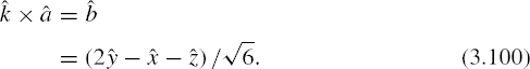
The basic polarization categories presented here for a wave propagating in the direction are also applicable for waves propagating in other directions. Consider the example

Here, we have a plane wave propagating in the direction, and it is easy to show that , so that the field is indeed perpendicular to the direction of propagation.

To classify the polarization of this plane wave, we need to resolve into two components perpendicular to each other and to :

Once the complex amplitudes and are determined, the polarization can be classified in a manner similar to that for the plane wave propagating only in the direction.

Choosing and is arbitrary, so to begin, any can be chosen that is perpendicular to . Here, we choose . Now can be determined, since we must have

Now

so that the two polarizations components have the same amplitude and are out of phase 90°: this is circular polarization.

The handedness of the circular polarization can be classified by plotting the field vector at a fixed point in space as time elapses. This implies returning to the time domain

with the second equation at a convenient location in space, namely, the origin. We see that at time zero, the field vector is pointing in the − direction, and then as time elapses the field traces out a circle in the direction at first of the − direction. Noting that , this is a left-hand circular polarization because one's right hand thumb points opposite the direction of propagation when the right hand fingers are circulated in the direction of the field vector rotation.

REFERENCES

1. Harrington, R. F., Time-Harmonic Electromagnetic Fields, McGraw-Hill, 1961.

2. Budden, K. G., The Propagation of Radio Waves, Cambridge University Press, 1985.

3. Chew, W. C., Waves and Fields in Inhomogeneous Media, IEEE Press, 1999.

4. Kong, J. A., Electromagnetic Wave Theory, EMW Publishing, 2008.