12

OTHER PROPAGATION MECHANISMS AND APPLICATIONS

12.1 INTRODUCTION

This chapter presents overviews of two of the more “unusual” propagation mechanisms (tropospheric and meteor scatter) mentioned briefly in Chapter 1, along with a discussion of propagation effects for two applications: tropospheric delays in satellite navigation systems and propagation effects on radar systems. While the material is presented only at an introductory level, it is intended to enable the reader to understand the basic aspects of these topics; sources of further information are also provided.

12.2 TROPOSPHERIC SCATTER

12.2.1 Introduction

At VHF and higher frequencies, the ionosphere is not a viable communications medium. In these frequency bands, the mode of signal transmission is characterized by three propagation mechanisms, depending on the distance, as sketched in Figure 12.1. For LOS conditions, the direct transmission mode of Chapter 5 is applicable, possibly with the addition of reflections from the ground, as discussed in Chapter 6. Beyond the radio horizon, diffraction (Chapter 7) takes over. The attenuation rate of the diffracted signal depends on the nature of the diffracting obstacle and is higher for relatively smooth ground than for a knife-edge-like mountain range. Even in the diffraction range of distances, another signal is present due to scatter from turbulent irregularities in the lower troposphere. At relatively short ranges, diffraction is dominant. Beyond some distance, which depends on both the diffracting obstacle and the tropospheric turbulence, the scattered signal becomes dominant and can be used for communication. Tropospheric scatter links can operate over long distances: as far as 1000 km for narrowband signals and up to 200–300 km for wider band signals [1]. However, signal fading on tropospheric scatter links is usually severe, and high-power transmitters, high-gain antennas, sensitive receivers, and often some form of diversity are needed to overcome fading problems. Limits on antenna sizes put the minimum practical frequency for “troposcatter” systems at around 200 MHz, while increasing losses with frequency and rain attenuation put an upper limit at approximately 5 GHz.

FIGURE 12.1 Typical plot of path attenuation versus distance d.

Since tropospheric scatter propagation depends on scattering from variations in the atmospheric refractivity, theoretical prediction of expected losses requires a very detailed knowledge of the local atmospheric structure. Obtaining such information is exceedingly difficult, given the wide variations in atmospheric properties that occur in time, location, and altitude. As a result, theoretical methods are of limited use in tropospheric scatter predictions. Measurements form the basis of the only available prediction models, which are empirical. Even their application to situations for which the measurements were not performed is of limited accuracy. To reduce uncertainties in empirical predictions, models are usually provided for the annual median loss along a tropospheric path, with additional information available on the fading rates to be expected.

The typical geometry of a tropospheric scatter link is illustrated in Figure 12.2. Stations beyond the line of sight direct their antennas near the horizon. The region that contains both the transmitting and receiving antenna beams, centered around the point C in the figure, is called the common volume. Atmospheric scatter that gives rise to the received signal results from this common volume. Measurements have shown that antennas should be directed 0.2–0.6 beamwidths above the horizon for optimal results due to the fact that the atmospheric irregularities that cause the scattering decrease with altitude. For simplicity, these antenna pointing angles are not shown in Figure 12.2, and they are not considered in the empirical model of Section 12.2.2 below.

FIGURE 12.2 Geometry of a tropospheric scatter link.

It is clear that fading should be expected on a tropospheric scatter link since the scattered signals originate from a large number of sources within the common volume, and the position of these scatterers changes in time as the atmosphere varies. It is also clear that the tropospheric scatter mechanism is dispersive since the phase shift obtained in scattering from individual atmospheric irregularities will vary with frequency. Thus tropospheric links are always narrowband, and transmissible bandwidths decrease from around 10 MHz at short ranges to less than 1 MHz at long ranges, due to the increased number of scatterers inside the common volume. High transmitted powers, sensitive receivers, large antennas, and diversity techniques allow these fades to be tolerated, however, and reliable links can be created. The antenna-to-medium coupling loss term L_coup, discussed in Chapter 5, also becomes significant because the received fields are not plane waves since they are due to contributions from many scatterers spread over a substantial field of view, not due to a distant point source. This loss places a limit on the increase in link performance that can be obtained by increasing antenna gains.

As with ionospheric communication systems, the relative importance of troposcatter for long-distance communications has diminished since the advent of satellite systems. Nevertheless, troposcatter systems are still used for some long-distance terrestrial links where it is not feasible or cost-effective to employ many repeater stations between the transmitter and receiver, such as in links over the ocean to distant offshore oil platforms or islands. Fixed and, more recently, mobile troposcatter systems are also of importance in military applications, either to augment existing satellite systems or to provide a back up mode of operation.

12.2.2 Empirical Model for the Median Path Loss

ITU-R Recommendation P.617-1 [2] provides an empirical estimate of the annual median path loss for troposcatter links. This estimate is based on data from 200 MHz to 4 GHz, and it is written in decibels as

where f is the frequency in MHz, d is the path length in kilometers, and θ is the scatter angle indicated in Figure 12.2, expressed in milliradians (mrad). The antenna-to-medium coupling loss L_coup is given by

where G_T and G_R are the transmitter and receiver antenna gains in dBi. The term N(H, h) also depends on the scatter angle and is given by

where H = 2.5 × 10⁻⁴ θd and h = 1.25 × 10⁻⁷ θ²R_e, with θ and d expressed in mrad and km, respectively, and where R_e = κa is the effective Earth radius for median refractive conditions, as discussed in Chapter 6, expressed in km. The meteorological structure parameter M depends on the local climate and varies between about 20 and 40 dB. The atmospheric structure parameter γ also depends on the climate and assumes values in the range 0.3 ± 0.03 km⁻¹. A table with values for M and γ in different climates can be found in Ref. [2]. Because the median path loss increases as θ increases, the antennas in a troposcatter link are generally positioned to minimize the scatter angle and maximize the common volume. Extensions of the annual median loss predictions of equation (12.1) to losses at other probabilities of occurrence are also described in Ref. [2].

12.2.3 Fading in Troposcatter Links

The above empirical model provides an estimate for the annual median path loss. In practice, the path loss in troposcatter links shows both daily and seasonal variations. Daily variations are caused by changes in tropospheric conditions such as pressure, moisture, and temperature. Similarly, seasonal variations occur as these conditions vary according to annual cycles. These seasonal variations depend on the local climate. In temperate climates, the path loss is larger during the winter; in desert climates, the path loss is larger during the summer. Path losses in equatorial climates have little seasonal variation. Regarding daily variations, the path loss is larger in the afternoon and decreases at night and in the morning [3].

Daily and seasonal variations correspond to a slow fading of the signal in decibels that can be described statistically in terms of a Gaussian distribution, as seen in Chapter 8. The variance of the slow fading tends to decrease as the path length increases because the common volume is then attained at higher altitudes, which show less daily variability in scatter properties than at lower altitudes. For a link with d = 80 km, the slow fading standard deviation is typically about 30 dB, whereas for d = 500 km, it decreases to around 10 dB [3]. Superimposed on the slow fading are short-term variations in the signal that can reach up to 20 fades per second. This fast fading is caused by fluctuations in the number, orientation, and position of the tropospheric fluctuations in the common volume, and is described statistically by a Rayleigh distribution (Chapter 8). Because fading in troposcatter links can be severe, diversity schemes become necessary. Spatial, frequency, and angle diversity can be used individually or in combination to combat troposcatter fading. For angle diversity, multiple antenna feeds can be spaced in the vertical direction to create multiple vertically spaced common volumes.

Tropospheric scattering can be a source of interference in other communication systems. In this case, the common volume can arise even from the intersection of the sidelobes of two antennas, or the sidelobe of one antenna and the mainlobe of a second antenna.

12.3 METEOR SCATTER

Meteors enter the Earth's upper atmosphere continually at speeds ranging from 10 to 75 km/s. At a height of approximately 120 km, meteors encounter an atmospheric density large enough that heat builds up between the meteor and the atmosphere to produce an ionization trail. These trails have an average length of 15 km but can reach up to 50 km.

Most of the meteors are quite small and disintegrate very quickly in the upper atmosphere. Nevertheless, it is estimated that about 10¹² meteors enter the atmosphere every day that can produce an ionization trail sufficient to be of use in reflecting radio signals. In general, meteors suitable for this purposes have a mass greater than 1 × 10⁻⁷ g [4].

There are two mechanisms of reflection of radio signals by meteor trails. In overdense trails, that is with ionization density above 2 × 10¹⁴ electrons/m, the trail core behaves as a plasma and the incident wave is reflected from the region of the trail where the plasma frequency equals the radiowave frequency. Underdense trails, that is, those with ionization density below the above threshold, do not reach a plasma state. In this case, the incident wave excites the individual electrons that then reradiate the signal as a collection of small dipoles. The peak ionization density of a meteor trail depends on the meteor mass. Typically, only meteors with mass 1 × 10⁻³ g or greater can produce overdense trails. Because of the diffusion of the electrons into the atmosphere, overdense trails grow in volume while the density decreases, eventually becoming underdense. The relaxation time associated with this diffusion process depends on the local atmospheric density.

Because the number of underdense trails vastly exceeds the number of overdense trails, the reflected signal in meteor scatter systems is primarily caused by the former. Communication systems relying on meteor scatter are designed as if all reflections were caused by underdense trails. Because the duration of usable individual trails is typically very short, ranging from tens of milliseconds to a few seconds, communication links that rely on meteor scatter are often called meteor burst communication (MBC) systems. MBC links typically can have ranges of up to 1800 km and their useful frequency range is typically between about 20 and 120 MHz. This frequency range is limited from below by ionospheric attenuation and the need to minimize interference from ionospheric links, and from above by the fact that the received power for underdense trail scattering decreases as f⁻³. The optimal performance occurs in the 40–55 MHz frequency range [5,6].

There is a seasonal and diurnal variability in the rate of incidence of meteors that produces a variability in MBC link performance. The highest incidence of meteors occurs at dawn and the lowest at sunset.¹ The reason is that the morning side of the Earth moves forward relative to the orbital movement around the Sun, whereas the evening side moves backward; therefore, more meteors are “swept” by the Earth in the morning. Seasonal variations of similar magnitude occur with a maximum flux rate in August and a minimum in February. This seasonal variation occurs because the Earth's orbit passes through a region of denser solar orbit material in August [5,6].

As already stated, MBC systems can only transmit bursts of data while a usable meteor trail is present. To determine when this is the case, each station continually sends a “probing” signal to the other station; when this signal is received, a suitable trail is present and data transmission can proceed. A usable trail must create at least approximately a specular reflection condition for the transmitter and receiver locations. When no usable trail is present, the transmission becomes idle (“wait time”). The wait time is much greater than the burst time: for burst durations of 0.1 s, the wait time is about 17 s on average; for burst durations of 0.4 s, it is about 140 s [7]. As a result, the average data rates are very small, in the range 10–300 bps, and MBC systems are incompatible with certain applications such as voice communications. On the other hand, they are relatively inexpensive for low data rate applications and can be deployed using a decentralized, mobile infrastructure with small antennas. Because of this, MBC systems are particularly suited for remote, nonintensive data collection. In the United States, the Department of Agriculture currently operates a MBC system called SNOTEL (“snow telemetry”) with over 500 sites for collection of snow depth and other climate data in remote unattended locations. In another application, the Alaskan MBC system is utilized by five U.S. federal agencies to collect data from remote areas in Alaska.

MBC systems also have interest in some military applications because the ground footprint of the meteor scatter signals is smaller than that of satellite or skywave systems. As a result, MBC links provide a higher level of covertness and good resistance to ground-based interference and jamming. Mobile MBC systems also hold strategic interest as a “high survivability” means of long-distance data communications: in the event of a nuclear conflict, communication systems based upon centralized or fixed stations (satellites, fixed troposcatter, etc.) would be primary targets, and the fallout present in the D layer of the atmosphere would likely disrupt ionospheric skywave links.

ITU-R Recommendation P.843-1 [6] provides useful information for the design and planning of MBC systems, including the estimation of useful burst rates, choice of operation frequencies, and antenna considerations.

12.4 TROPOSPHERIC DELAY IN GLOBAL SATELLITE NAVIGATION SYSTEMS

Global navigation systems such as GPS are based on time delay measurements of signals broadcast by satellites and received by ground or aircraft users. The measured time delays are affected by variations in the refractive index n of the troposphere. Because n > 1, there is an excess time delay compared to propagation in a vacuum that can be quite significant, ranging from 6 to 80 ns (corresponding to 2–25 m range differences for GPS systems).² Errors due to these delays must be compensated if high-precision positional information is to be achieved [8]. In Chapter 11, we have examined an analogous excess delay in GPS signals caused by the ionosphere. Because the ionospheric delay is dispersive at L band, it can be compensated using dual-frequency receivers: GPS systems use a primary signal (L1) at 1575.42 MHz and a secondary signal (L2) at 1227.60 MHz. Unfortunately, this solution is of no use to compensate the tropospheric delay because the troposphere is not dispersive for frequencies below 15 GHz.

The tropospheric delay is written in terms of the refractive index n as

where c is the speed of light, and ds is the infinitesimal length along the propagation path S from the satellite to the receiver; c and ds should be in compatible units in this equation (typically m/s and m, with the delay in seconds). Because of refraction, the actual propagation path is curved and hence longer than the geometrical (straight) path length from the satellite to the receiver. The delay along the geometrical path when no tropospheric effects are present is given by

where S_s is a straight line from the satellite to the receiver. The excess delay time is Δt^e = Δt^a − Δt^s, that is,

This last equation can be rewritten as

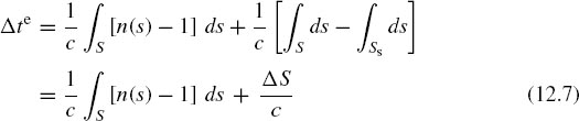
or

with the refractive index N(s) expressed in “N-units,” as seen in Chapter 6, and where ΔS is the difference in length between actual and straight paths. Sometimes, the term “tropospheric delay” is used to refer to the time delay above multiplied by the speed of light, that is, the length c Δt^e. The tropospheric delay is more pronounced for lower elevation angles (i.e., with the satellite near the horizon) than for large elevation angles (satellite near zenith) because of the longer path length through the troposphere in the former case.

It is convenient to separate two contributions to the tropospheric delay at L band: the dry delay, caused by dry gases (mostly nitrogen and oxygen), and the wet delay, caused by water vapor. The dry delay typically accounts for 90% or more of the total tropospheric delay. Because the dry atmosphere has a very uniform composition (with the exception of CO₂, which makes a negligible contribution), the dry delay can be modeled with a higher degree of predictability as a function of the local ground temperature and atmospheric pressure. In contrast, the water vapor content is highly variable in altitude, geographical location, and time, making it more difficult to model even when local ground humidity data are available.

The tropospheric delay can be written in terms of a sum of dry delay and wet delay contributions as

where ΔS_zd and ΔS_zw are the dry and wet delay, respectively, at zenith, while m_d(θ) and m_w(θ) are dry and wet “mapping functions” (obliquity factors), respectively, that model increases in the tropospheric delay as the elevation angle θ decreases. The mapping functions depend on both θ and the atmospheric profile of the refractive index, but for simplicity many approximate predictive models assume dependence only on θ.

Predictive models for the tropospheric delay can be obtained in two ways. One way is to determine the atmospheric profile from measurements and calculate the refractive index of each layer of the troposphere. Once the refractive index profile is known, the delay can be found using ray tracing. The atmospheric profile consists of measurements of temperature, pressure, and water vapor density for varying altitudes. The most sophisticated models are based on numerical weather model data [9]. This approach gives more precise results but it has two drawbacks: first, a typical user rarely has access to such measurements, and second, it is computationally intensive [10]. Another way to find the tropospheric delay is to use empirical models for the combined zenith delay due to both dry and wet components, which rely on either the seasonal average of weather parameters or actual delay measurement data at the receiver location, augmented by mapping functions to model the effect of longer propagation paths for satellites at lower elevation angles [9,10].

One of the simplest approximate models [8] is based on a fit of annual average delay data obtained using U.S. Standard Atmosphere parameters (Chapter 10) at 30°N, 45°N, 60°N latitude and ray tracing. It predicts a combined zenith delay

in meters and mapping functions of the form

so that

in units of meters for a receiver at sea level (h = 0). This approximate model gives a value of cΔt^e(0) = 2.44 m at zenith (θ = 90°) and cΔt^e(0) = 24.9 m for a 5° elevation angle. By further assuming that the refractivity varies with altitude approximately as (1 − h/h_d)⁴ with h in km and h_d = 43 km, the following approximation [8] can be obtained for the delay in meters for a receiver at altitude h:

This simplified model gives only a rough estimate of the tropospheric delay. Also, neither short-term variations affecting the wet delay component nor seasonal/geographical variations are included.

The term “tropospheric delay” is somewhat of a misnomer because about a quarter of the nonionized delay actually occurs due to atmospheric gases above the troposphere, that is, in the tropopause and stratosphere. Note that the troposphere also produces attenuation of GPS signals at L band, mainly due to oxygen absorption. However, this attenuation is generally small at GPS frequencies: no greater than 0.5 dB for satellites at low elevation angles and 0.05 dB for satellites near zenith [3].

12.5 PROPAGATION EFFECTS ON RADAR SYSTEMS

Radar (radio detection and ranging) systems attempt to determine information about remote targets by transmitting electromagnetic waves and measuring properties of the signals that are returned. Radars are routinely used for tracking of aircraft and ships; for collision avoidance, aircraft guidance, and landing-assistance systems; for determination of weather patterns, terrain altitude, and snow cover thickness; for underground exploration of minerals, gas, and oil; and in many other applications. Radar systems can be classified as either monostatic or bistatic. In monostatic radar, the transmitting and receiving antennas are colocated, whereas in bistatic radar, the transmitting and receiving antennas are in different locations.

In many applications, information about the remote region or target is sought from the power level of the returned signal, that is, the “target echo”. To quantify this process, we first consider monostatic radar and propagation in free space for simplicity. Assuming that a discrete target is present in the far field at distance R and look angle (θ, φ) from the radar, we can use equation (5.2) to write the power density (Poynting vector magnitude) of the field incident on the target as

where P_T is the total input power to the transmitter antenna and G_T is the transmitter antenna gain. The basic parameter that describes the reflectivity of the target is the radar cross section (RCS), denoted as σ_RCS. The RCS is an area such that the product S_T(R, θ, φ) σ_RCS (watts) is equal to the radiated power of an equivalent isotropic radiator at the target location that would produce the same power density S_R as observed at the radar receiver antenna. In other words,

Mathematically, the RCS of a target can also be expressed as the (far-field) limit

where is the electric field incident on the target and is the far-field scattered electric field from the target. Among the factors that may influence the RCS are the target's size, shape, and material (constitutive) properties. In general, the RCS also depends on the relative orientation of the target with respect to the direction of propagation of the incident wave, as well as on the polarization of the incident wave. Since the target is assumed to be in the far field of the radar, the RCS does not depend on the range R.

Using equation (12.15), the received power for a receiving antenna with effective aperture area A_R can be found as

Combining equations (12.14) and (12.17), and using the fact that A_R = λ²G_R/(4π), we obtain the monostatic radar equation

where G_R is the receiver antenna gain and λ is the wavelength of operation. Note that when the same antenna is used for transmitting and receiving in monostatic radar, G_T(θ, φ) = G_R(θ, φ). In contrast to the Friis transmission formula, which applies to one-way transmissions,—equation (5.5)—the received power in the radar equation decays as 1/R⁴ instead of 1/R².

Rearranging some factors, we can also rewrite equation (12.18) as

which, when expressed in decibels, becomes

where is the free-space path loss in decibels, given by

For propagation scenarios where the use of the free-space path loss is not justified, should be replaced by the appropriate path loss model L_p, that is,

Free-space propagation is often assumed in many radar analyses; it is important to recognize when this is appropriate and when it is not. It is also common to see equation (12.22) written as

where F is a factor that describes any propagation gain relative to free space (note that F can be either positive or negative).

When bistatic radar is considered, equation (12.22) is modified to

where (θ_T, φ_T), (θ_R, φ_R) are the look angles from the transmitter and receiver antennas to the target, respectively, while L_p,T and L_p,R are the path losses from the target to the transmitter and receiver antennas, respectively. Here, represents the bistatic RCS of the target, which depends on the bistatic angle (the angle between the transmitter and the receiver, as seen from the target location) and the orientation of the target.

Radar engineering is a vast and fascinating topic, and further discussion on this subject is beyond the objectives of this book. A good introduction to this topic can be found in Ref. [11].

REFERENCES

1. M. P. M. Hall, Effects of the Troposphere on Radio Communication, Peter Peregrinus Ltd., 1979.

2. ITU-R Recommendation P.617-1, “Propagation prediction techniques and data required for the design of trans-horizon radio-relay systems,” International Telecommunication Union, 1992.

3. Bothias, L., Radiowave Propagation, Section 8.1.1.3, McGraw-Hill, 1987.

4. Sugar, G. R., “Radio propagation by reflection from meteor trails,” Proc. IEEE, vol. 52, pp. 116–136, 1964.

5. Freeman, R. L., Radio System Design for Telecommunications, Chapter 13, third edition, Wiley–IEEE Press, 2007.

6. ITU-R Recommendation P.843-1, “Communication by meteor burst propagation,” International Telecommunication Union, 1997.

7. “Meteor burst communications: An ignored phenomenon?”, Cryptologic Quarterly, vol. 9, no. 3, pp. 47–63, 1990.

8. Spiker Jr., J. J., “Tropospheric effects on GPS,” in Global Positioning System: Theory and Applications, Volume 1, pp. 517–546, (Progress in Astronautics and Aeronautics vol. 163), AIAA, Washington DC, 1996.

9. Boehm, J., A. E. Niell, P. Tregoning, and H. Schuh, “Global mapping function (GMF): a new empirical mapping function based on numerical weather model data,” Geophys. Res. Lett., vol. 33, no. 7, p. L07304, 2006.

10. Hobiger, T., R. Ichikawa, Y. Koyama, and T. Kondo, “Computation of troposphere slant delays on a GPU,” IEEE Trans. Geosci. Remote Sens., vol. 47, no. 10, 2009.

11. Skolnik, M., Introduction to Radar Systems, third edition, McGraw-Hill, 2002.