CHAPTER 10

VARIABLE SELECTION AND MODEL BUILDING

10.1 INTRODUCTION

10.1.1 Model-Building Problem

In the preceding chapters we have assumed that the regressor variables included in the model are known to be important. Our focus was on techniques to ensure that the functional form of the model was correct and that the underlying assumptions were not violated. In some applications theoretical considerations or prior experience can be helpful in selecting the regressors to be used in the model.

In previous chapters, we have employed the classical approach to regression model selection, which assumes that we have a very good idea of the basic form of the model and that we know all (or nearly all) of the regressors that should be used. Our basic strategy is as follows:

1. Fit the full model (the model with all of the regressors under consideration).
2. Perform a thorough analysis of this model, including a full residual analysis. Often, we should perform a thorough analysis to investigate possible collinearity.
3. Determine if transformations of the response or of some of the regressors are necessary.
4. Use the t tests on the individual regressors to edit the model.
5. Perform a thorough analysis of the edited model, especially a residual analysis, to determine the model's adequacy.

In most practical problems, especially those involving historical data, the analyst has a rather large pool of possible candidate regressors, of which only a few are likely to be important. Finding an appropriate subset of regressors for the model is often called the variable selection problem.

Good variable selection methods are very important in the presence of multicollinearity. Frankly, the most common corrective technique for multicollinearity is variable selection. Variable selection does not guarantee elimination of multicollinearity. There are cases where two or more regressors are highly related; yet, some subset of them really does belong in the model. Our variable selection methods help to justify the presence of these highly related regressors in the final model.

Multicollinearity is not the only reason to pursue variable selection techniques. Even mild relationships that our multicollinearity diagnostics do not flag as problematic can have an impact on model selection. The use of good model selection techniques increases our confidence in the final model or models recommended.

Building a regression model that includes only a subset of the available regressors involves two conflicting objectives. (1) We would like the model to include as many regressors as possible so that the information content in these factors can influence the predicted value of y. (2) We want the model to include as few regressors as possible because the variance of the prediction increases as the number of regressors increases. Also the more regressors there are in a model, the greater the costs of data collection and model maintenance. The process of finding a model that is a compromise between these two objectives is called selecting the “best” regression equation. Unfortunately, as we will see in this chapter, there is no unique definition of “best.” Furthermore, there are several algorithms that can be used for variable selection, and these procedures frequently specify different subsets of the candidate regressors as best.

The variable selection problem is often discussed in an idealized setting. It is usually assumed that the correct functional specification of the regressors is known (e.g., 1/x₁, ln x₂) and that no outliers or influential observations are present. In practice, these assumptions are rarely met. Residual analysis, such as described in Chapter 4, is useful in revealing functional forms for regressors that might be investigated, in pointing out new candidate regressors, and for identifying defects in the data such as outliers. The effect of influential or high-leverage observations should also be determined. Investigation of model adequacy is linked to the variable selection problem. Although ideally these problems should be solved simultaneously, an iterative approach is often employed, in which (1) a particular variable selection strategy is employed and then (2) the resulting subset model is checked for correct functional specification, outliers, and influential observations. This may indicate that step 1 must be repeated. Several iterations may be required to produce an adequate model.

None of the variable selection procedures described in this chapter are guaranteed to produce the best regression equation for a given data set. In fact, there usually is not a single best equation but rather several equally good ones. Because variable selection algorithms are heavily computer dependent, the analyst is sometimes tempted to place too much reliance on the results of a particular procedure. Such temptation is to be avoided. Experience, professional judgment in the subject-matter field, and subjective considerations all enter into the variable selection problem. Variable selection procedures should be used by the analyst as methods to explore the structure of the data. Good general discussions of variable selection in regression include Cox and Snell [1974], Hocking [1972, 1976], Hocking and LaMotte [1973], Myers [1990], and Thompson [1978a, b].

10.1.2 Consequences of Model Misspecification

To provide motivation for variable selection we will briefly review the consequences of incorrect model specification. Assume that there are K candidate regressors x₁, x₂, …, x_K and n ≥ K + 1 observations on these regressors and the response y. The full model, containing all K regressors, is

or equivalently

We assume that the list of candidate regressors contains all the important variables. Note that Eq. (10.1) contains an intercept term β₀. While β₀ could also be a candidate for selection, it is typically forced into the model. We assume that all equations include an intercept term. Let r be the number of regressors that are deleted from Eq. (10.1). Then the number of variables that are retained is p = K + 1 − r. Since the intercept is included, the subset model contains p − 1 = K − r of the original regressors.

The model (10.1) may be written as

where the X matrix has been partitioned into X_p, an n × p matrix whose columns represent the intercept and the p − 1 regressors to be retained in the subset model, and X_r, an n × r matrix whose columns represent the regressors to be deleted from the full model. Let β be partitioned conformably into β_p and β_r. For the full model the least-squares estimate of β is

and an estimate of the residual variance σ² is

The components of are denoted by denotes the fitted values.

For the subset model

the least-squares estimate of β_p is

the estimate of the residual variance is

and the fitted values are ŷ_i.

The properties of the estimates from the subset model have been investigated by several authors, including Hocking [1974, 1976], Narula and Ramberg [1972], Rao [1971], Rosenberg and Levy [1972], and Walls and Weeks [1969].

The results can be summarized as follows:

1. The expected value of is

   

   where A = (X_p′X_p)⁻¹ X_p′X_r (A is sometimes called the alias matrix). Thus, is a biased estimate of β_p unless the regression coefficients corresponding to the deleted variables (β_r) are zero or the retained variables are orthogonal to the deleted variables (X_p′X_r = 0).

2. The variances of and are Var () = σ² (X_p′X_p)⁻¹ and Var () = σ² (X′X)⁻¹,

   respectively. Also the matrix Var − Var () is positive semidefinite, that is, the variances of the least-squares estimates of the parameters in the full model are greater than or equal to the variances of the corresponding parameters in the subset model. Consequently, deleting variables never increases the variances of the estimates of the remaining parameters.

3. Since is a biased estimate of β _p and is not, it is more reasonable to compare the precision of the parameter estimates from the full and subset models in terms of mean square error. Recall that if is an estimate of the parameter θ, the mean square error of is

   

   The mean square error of is

   

   If the matrix is positive semidefinite, the matrix is positive semidefinite. This means that the least-squares estimates of the parameters in the subset model have smaller mean square error than the corresponding parameter estimates from the full model when the deleted variables have regression coefficients that are smaller than the standard errors of their estimates in the full model.

4. The parameter from the full model is an unbiased estimate of σ². However, for the subset model

   

   That is, is generally biased upward as an estimate of σ².

5. Suppose we wish to predict the response at the point X′ = [X′_p, x′_r]. If we use the full model, the predicted value is , with mean x′β and prediction variance

   

   However, if the subset model is used, with mean

   

   and prediction mean square error

   

   Note that ŷ is a biased estimate of y unless x′_pAβ_r = 0, which is only true in general if X′_pX_rβ_r = 0. Furthermore, the variance of ŷ* from the full model is not less than the variance of ŷ from the subset model. In terms of mean square error we can show that

   

   provided that the matrix is positive semidefinite.

Our motivation for variable selection can be summarized as follows. By deleting variables from the model, we may improve the precision of the parameter estimates of the retained variables even though some of the deleted variables are not negligible. This is also true for the variance of a predicted response. Deleting variables potentially introduces bias into the estimates of the coefficients of retained variables and the response. However, if the deleted variables have small effects, the MSE of the biased estimates will be less than the variance of the unbiased estimates. That is, the amount of bias introduced is less than the reduction in the variance. There is danger in retaining negligible variables, that is, variables with zero coefficients or coefficients less than their corresponding standard errors from the full model. This danger is that the variances of the estimates of the parameters and the predicted response are increased.

Finally, remember from Section 1.2 that regression models are frequently built using retrospective data, that is, data that have been extracted from historical records. These data are often saturated with defects, including outliers, “wild” points, and inconsistencies resulting from changes in the organization's data collection and information-processing system over time. These data defects can have great impact on the variable selection process and lead to model misspecification. A very common problem in historical data is to find that some candidate regressors have been controlled so that they vary over a very limited range. These are often the most influential variables, and so they were tightly controlled to keep the response within acceptable limits. Yet because of the limited range of the data, the regressor may seem unimportant in the least-squares fit. This is a serious model misspecification that only the model builder's nonstatistical knowledge of the problem environment may prevent. When the range of variables thought to be important is tightly controlled, the analyst may have to collect new data specifically for the model-building effort. Designed experiments are helpful in this regard.

10.1.3 Criteria for Evaluating Subset Regression Models

Two key aspects of the variable selection problem are generating the subset models and deciding if one subset is better than another. In this section we discuss criteria for evaluating and comparing subset regression models. Section 10.2 will present computational methods for variable selection.

Coefficient of Multiple Determination A measure of the adequacy of a regression model that has been widely used is the coefficient of multiple determination, R². Let R_p² denote the coefficient of multiple determination for a subset regression model with p terms, that is, p − 1 regressors and an intercept term β₀. Computationally,

where SS_R(p) and SS_Res(p) denote the regression sum of squares and the residual sum of squares, respectively, for a p-term subset model. Note that there are values of R_p² for each value of p, one for each possible subset model of size p. Now R_p² increases as p increases and is a maximum when p = K + 1. Therefore, the analyst uses this criterion by adding regressors to the model up to the point where an additional variable is not useful in that it provides only a small increase in R_p². The general approach is illustrated in Figure 10.1, which presents a hypothetical plot of the maximum value of R_p² for each subset of size p against p. Typically one examines a display such as this and then specifies the number of regressors for the final model as the point at which the “knee” in the curve becomes apparent. Clearly this requires judgment on the part of the analyst.

Since we cannot find an “optimum” value of R² for a subset regression model, we must look for a “satisfactory” value. Aitkin [1974] has proposed one solution to this problem by providing a test by which all subset regression models that have an R² not significantly different from the R² for the full model can be identified. Let

Figure 10.1 Plot of R_p² versus p.

where

and R²_k+1 is the value of R² for the full model. Aitkin calls any subset of regressor variables producing an R² greater than R²₀ an R²-adequate (α) subset.

Generally, it is not straightforward to use R² as a criterion for choosing the number of regressors to include in the model. However, for a fixed number of variables p, R_p² can be used to compare the subset models so generated. Models having large values of R_p² are preferred.

Adjusted R² To avoid the difficulties of interpreting R², some analysts prefer to use the adjusted R² statistic, defined for a p-term equation as

The statistic does not necessarily increase as additional regressors are introduced into the model. In fact, it can be shown (Edwards [1969], Haitovski [1969], and Seber [1977]) that if s regressors are added to the model, will exceed if and only if the partial F statistic for testing the significance of the s additional regressors exceeds 1. Consequently, one criterion for selection of an optimum subset model is to choose the model that has a maximum . However, this is equivalent to another criterion that we now present.

Residual Mean Square The residual mean square for a subset regression model, for example,

may be used as a model evaluation criterion. The general behavior of MS_Res(p) as p increases is illustrated in Figure 10.2. Because SS_Res(p) always decreases as p increases, MS_Res(p) initially decreases, then stabilizes, and eventually may increase. The eventual increase in MS_Res(p) occurs when the reduction in SS_Res(p) from adding a regressor to the model is not sufficient to compensate for the loss of one degree of freedom in the denominator of Eq. (10.11). That is, adding a regressor to a p-term model will cause MS_Res(p + 1) to be greater than MS_Res(p) if the decrease in the residual sum of squares is less than MS_Res(p). Advocates of the MS_Res(p) criterion will plot MS_Res(p) versus p and base the choice of p on the following:

Figure 10.2 Plot of MS_Res (p) versus p.

1. The minimum MS_Res(p)
2. The value of p such that MS_Res(p) is approximately equal to MS_Res for the full model
3. A value of p near the point where the smallest MS_Res(p) turns upward

The subset regression model that minimizes MS_Res(p) will also maximize . To see this, note that

Thus, the criteria minimum MS_Res(p) and maximum adjusted R² are equivalent.

Mallows's C_p Statistic Mallows [1964, 1966, 1973, 1995] has proposed a criterion that is related to the mean square error of a fitted value, that is,

Note that E(y_i) is the expected response from the true regression equation and E(ŷ_i) is the expected response from the p-term subset model. Thus, is the bias at the ith data point. Consequently, the two terms on the right-hand side of Eq. (10.12) are the squared bias and variance components, respectively, of the mean square error. Let the total squared bias for a p-term equation be

and define the standardized total mean square error as

It can be shown that

and that the expected value of the residual sum of squares from a p-term equation is

Substituting for and SS_B(p) in Eq. (10.13) gives

Suppose that is a good estimate of σ². Then replacing E[SS_Res(p)] by the observed value SS_Res(p) produces an estimate of Γ_p, say

If the p-term model has negligible bias, then SS_B(p) = 0. Consequently, E[SS_Res(p)] = (n − p)σ², and

When using the C_p criterion, it can be helpful to visualize the plot of C_p as a function of p for each regression equation, such as shown in Figure 10.3. Regression equations with little bias will have values of C_p that fall near the line C_p = p (point A in Figure 10.3) while those equations with substantial bias will fall above this line (point B in Figure 10.3). Generally, small values of C_p are desirable. For example, although point C in Figure 10.3 is above the line C_p = p, it is below point A and thus represents a model with lower total error. It may be preferable to accept some bias in the equation to reduce the average error of prediction.

To calculate C_p, we need an unbiased estimate of σ². Frequently we use the residual mean square for the full equation for this purpose. However, this forces C_p = p = K + 1 for the full equation. Using MS_Res(K + 1) from the full model as an estimate of σ² assumes that the full model has negligible bias. If the full model has several regressors that do not contribute significantly to the model (zero regression coefficients), then MS_Res(K + 1) will often overestimate σ², and consequently the values of C_p will be small. If the C_p statistic is to work properly, a good estimate of σ² must be used. As an alternative to MS_Res(K + 1), we could base our estimate of σ² on pairs of points that are “near neighbors” in x space, as illustrated in Section 4.5.2.

Figure 10.3 A C_p plot.

The Akaike Information Criterion and Bayesian Analogues (BICs) Akaike proposed an information criterion, AIC, based on maximizing the expected entropy of the model. Entropy is simply a measure of the expected information, in this case the Kullback-Leibler information measure. Essentially, the AIC is a penalized log-likelihood measure. Let L be the likelihood function for a specific model. The AIC is

where p is the number of parameters in the model. In the case of ordinary least squares regression,

The key insight to the AIC is similar to R²_Adj and Mallows C_p. As we add regressors to the model, SS_Res, cannot increase. The issue becomes whether the decrease in SS_Res justifies the inclusion of the extra terms.

There are several Bayesian extensions of the AIC. Schwartz (1978) and Sawa (1978) are two of the more popular ones. Both are called BIC for Bayesian information criterion. As a result, it is important to check the fine print on the statistical software that one uses! The Schwartz criterion (BIC_Sch) is

This criterion places a greater penalty on adding regressors as the sample size increases. For ordinary least squares regression, this criterion is

R uses this criterion as its BIC. SAS uses the Sawa criterion, which involves a more complicated penalty term. This penalty term involves σ² and σ⁴, which SAS estimates by MS_Res from the full model.

The AIC and BIC criteria are gaining popularity. They are much more commonly used in the model selection procedures involving more complicated modeling situations than ordinary least squares, for example, the mixed model situation outlined in Section 5.6. These criteria are very commonly used with generalized linear models (Chapter 13).

Uses of Regression and Model Evaluation Criteria As we have seen, there are several criteria that can be used to evaluate subset regression models. The criterion that we use for model selection should certainly be related to the intended use of the model. There are several possible uses of regression, including (1) data description, (2) prediction and estimation, (3) parameter estimation, and (4) control.

If the objective is to obtain a good description of a given process or to model a complex system, a search for regression equations with small residual sums of squares is indicated. Since SS_Res is minimized by using all K candidate regressors, we usually prefer to eliminate some variables if only a small increase in SS_Res results. In general, we would like to describe the system with as few regressors as possible while simultaneously explaining the substantial portion of the variability in y.

Frequently, regression equations are used for prediction of future observations or estimation of the mean response. In general, we would like to select the regressors such that the mean square error of prediction is minimized. This usually implies that regressors with small effects should be deleted from the model. One could also use the PRESS statistic introduced in Chapter 4 to evaluate candidate equations produced by a subset generation procedure. Recall that for a p-term regression model

One then selects the subset regression model based on a small value of PRESS_p. While PRESS_p has intuitive appeal, particularly for the prediction problem, it is not a simple function of the residual sum of squares, and developing an algorithm for variable selection based on this criterion is not straightforward. This statistic is, however, potentially useful for discriminating between alternative models, as we will illustrate.

If we are interested in parameter estimation, then clearly we should consider both the bias that results from deleting variables and the variances of the estimated coefficients. When the regressors are highly multicollinear, the least-squares estimates of the individual regression coefficients may be extremely poor, as we saw in Chapter 9.

When a regression model is used for control, accurate estimates of the parameters are important. This implies that the standard errors of the regression coefficients should be small. Furthermore, since the adjustments made on the x's to control y will be proportional to the , the regression coefficients should closely represent the effects of the regressors. If the regressors are highly multicollinear, the may be very poor estimates of the effects of individual regressors.

10.2 COMPUTATIONAL TECHNIQUES FOR VARIABLE SELECTION

We have seen that it is desirable to consider regression models that employ a subset of the candidate regressor variables. To find the subset of variables to use in the final equation, it is natural to consider fitting models with various combinations of the candidate regressors. In this section we will discuss several computational techniques for generating subset regression models and illustrate criteria for evaluation of these models.

10.2.1 All Possible Regressions

This procedure requires that the analyst fit all the regression equations involving one candidate regressor, two candidate regressors, and so on. These equations are evaluated according to some suitable criterion and the “best” regression model selected. If we assume that the intercept term β₀ is included in all equations, then if there are K candidate regressors, there are 2^K total equations to be estimated and examined. For example, if K = 4, then there are 2⁴ = 16 possible equations, while if K = 10, there are 2¹⁰ = 1024 possible regression equations. Clearly the number of equations to be examined increases rapidly as the number of candidate regressors increases. Prior to the development of efficient computer codes, generating all possible regressions was impractical for problems involving more than a few regressors. The availability of high-speed computers has motivated the development of several very efficient algorithms for all possible regressions. We illustrate Minitab and SAS in this chapter. The R function leaps() in the leaps directory performs an all possible regressions methodology.

Example 10.1 The Hald Cement Data

Hald [1952]^† presents data concerning the heat evolved in calories per gram of cement (y) as a function of the amount of each of four ingredients in the mix: tricalcium aluminate (x₁), tricalcium silicate (x₂), tetracalcium alumino ferrite (x₃), and dicalcium silicate (x₄). The data are shown in Appendix Table B.21. These reflect quite serious problems with multicollinearity. The VIFs are:

x1: 38.496

x2: 254.423

x3: 46.868

x4: 282.513

We will use these data to illustrate the all-possible-regressions approach to variable selection.

TABLE 10.1 Summary of All Possible Regressions for the Hald Cement Data

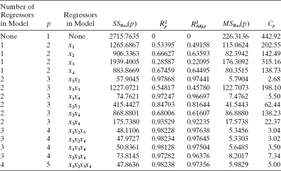
TABLE 10.2 Least-Squares Estimates for All Possible Regressions (Hald Cement Data)

Since there are K = 4 candidate regressors, there are 2⁴ = 16 possible regression equations if we always include the intercept β₀. The results of fitting these 16 equations are displayed in Table 10.1. The R_p², R²_Adj, p, MS_Res(p), and C_p statistics are also given in this table.

Table 10.2 displays the least-squares estimates of the regression coefficients. The partial nature of regression coefficients is readily apparent from examination of this table. For example, consider x₂. When the model contains only x₂, the least-squares estimate of the x₂ effect is 0.789. If x₄ is added to the model, the x₂ effect is 0.311, a reduction of over 50%. Further addition of x₃ changes the x₂ effect to −0.923. Clearly the least-squares estimate of an individual regression coefficient depends heavily on the other regressors in the model. The large changes in the regression coefficients observed in the Hald cement data are consistent with a serious problem with multicollinearity.

Figure 10.4 Plot of R_p² versus p, Example 10.1

Consider evaluating the subset models by the R_p² criterion. A plot of R_p² versus p is shown in Figure 10.4. From examining this display it is clear that after two regressors are in the model, there is little to be gained in terms of R² by introducing additional variables. Both of the two-regressor models (x₁, x₂) and (x₁, x₄) have essentially the same R² values, and in terms of this criterion, it would make little difference which model is selected as the final regression equation. It may be preferable to use (x₁, x₄) because x₄ provides the best one-regressor model. From Eq. (10.9) we find that if we take α = 0.05,

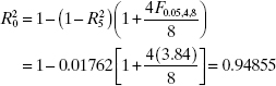
Therefore, any subset regression model for which is R² adequate (0.05); that is, its R² is not significantly different from R²_K+1. Clearly, several models in Table 10.1 satisfy this criterion, and so the choice of the final model is still not clear.

TABLE 10.3 Matrix of Simple Correlations for Hald's Data in Example 10.1

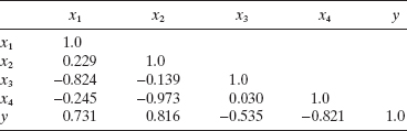
It is instructive to examine the pairwise correlations between x_i and x_j and between x_i and y. These simple correlations are shown in Table 10.3. Note that the pairs of regressors (x₁, x₃) and (x₂, x₄) are highly correlated, since

Consequently, adding further regressors when x₁ and x₂ or when x₁ and x₄ are already in the model will be of little use since the information content in the excluded regressors is essentially present in the regressors that are in the model. This correlative structure is partially responsible for the large changes in the regression coefficients noted in Table 10.2.

A plot of MS_Res(p) versus p is shown in Figure 10.5. The minimum residual mean square model is (x₁, x₂, x₄), with MS_Res (4) = 5.3303. Note that, as expected, the model that minimizes MS_Res (p) also maximizes the adjusted R². However, two of the other three-regressor models [(x₁, x₂, x₃) and (x₁, x₃, x₄)] and the two-regressor models [(x₁, x₂) and (x₁, x₄)] have comparable values of the residual mean square. If either (x₁, x₂) or (x₁, x₄) is in the model, there is little reduction in residual mean square by adding further regressors. The subset model (x₁, x₂) may be more appropriate than (x₁, x₄) because it has a smaller value of the residual mean square.

A C_p plot is shown in Figure 10.6. To illustrate the calculations, suppose we take = 5.9829 (MS_Res from the full model) and calculate C₃ for the model (x₁, x₄). From Eq. (10.15) we find that

From examination of this plot we find that there are four models that could be acceptable: (x₁, x₂), (x₁, x₂, x₃), (x₁, x₂, x₄), and (x₁, x₃, x₄). Without considering additional factors such as technical information about the regressors or the costs of data collection, it may be appropriate to choose the simplest model (x₁, x₂) as the final model because it has the smallest C_p.

This example has illustrated the computational procedure associated with model building with all possible regressions. Note that there is no clear-cut choice of the best regression equation. Very often we find that different criteria suggest different equations. For example, the minimum C_p equation is (x₁, x₂) and the minimum MS_Res equation is (x₁, x₂, x₄). All “final” candidate models should be subjected to the usual tests for adequacy, including investigation of leverage points, influence, and multicollinearity. As an illustration, Table 10.4 examines the two models (x₁, x₂) and (x₁, x₂, x₄) with respect to PRESS and their variance inflation factors (VIFs). Both models have very similar values of PRESS (roughly twice the residual sum of squares for the minimum MS_Res equation), and the R² for prediction computed from PRESS is similar for both models. However, x₂ and x₄ are highly multicollinear, as evidenced by the larger variance inflation factors in (x₁, x₂, x₄). Since both models have equivalent PRESS statistics, we would recommend the model with (x₁, x₂) based on the lack of multicollinearity in this model.

Figure 10.5 Plot of MS_Res (p) versus p, Example 10.1.

Efficient Generation of All Possible Regressions There are several algorithms potentially useful for generating all possible regressions. For example, see Furnival [1971], Furnival and Wilson [1974], Gartside [1965, 1971], Morgan and Tatar [1972], and Schatzoff, Tsao, and Fienberg [1968]. The basic idea underlying all these algorithms is to perform the calculations for the 2^K possible subset models in such a way that sequential subset models differ by only one variable. This allows very efficient numerical methods to be used in performing the calculations. These methods are usually based on either Gauss–Jordan reduction or the sweep operator (see Beaton [1964] or Seber [1977]). Some of these algorithms are available commercially. For example, the Furnival and Wilson [1974] algorithm is an option in the MlNlTAB and SAS computer programs.

Figure 10.6 The C_p plot for Example 10.1.

A sample computer output for Minitab applied to the Hald cement data is shown in Figure 10.7. This program allows the user to select the best subset regression model of each size for 1 ≤ p ≤ K + 1 and displays the C_p, R_p², and MS_Res(p) criteria. It also displays the values of the C_p, R_p², R²_Adj,p and statistics for several (but not all) models for each value of p. The program has the capability of identifying the m best (for m ≤ 5) subset regression models.

Current all-possible-regression procedures will very efficiently process up to about 30 candidate regressors with computing times that are comparable to the usual stepwise-type regression algorithms discussed in Section 10.2.2. Our experience indicates that problems with 30 or less candidate regressors can usually be solved relatively easily with an all-possible-regressions approach.

TABLE 10.4 Comparisons of Two Models for Hald's Cement Data

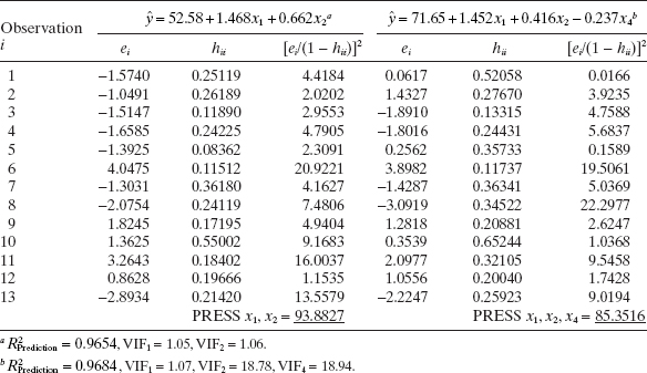
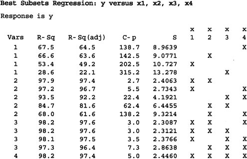
Figure 10.7 Computer output (Minitab) for Furnival and Wilson all-possible-regression algorithm.

10.2.2 Stepwise Regression Methods

Because evaluating all possible regressions can be burdensome computationally, various methods have been developed for evaluating only a small number of subset regression models by either adding or deleting regressors one at a time. These methods are generally referred to as stepwise-type procedures. They can be classified into three broad categories: (1) forward selection, (2) backward elimination, and (3) stepwise regression, which is a popular combination of procedures 1 and 2. We now briefly describe and illustrate these procedures.

Forward Selection This procedure begins with the assumption that there are no regressors in the model other than the intercept. An effort is made to find an optimal subset by inserting regressors into the model one at a time. The first regressor selected for entry into the equation is the one that has the largest simple correlation with the response variable y. Suppose that this regressor is x₁. This is also the regressor that will produce the largest value of the F statistic for testing significance of regression. This regressor is entered if the F statistic exceeds a preselected F value, say F_IN (or F-to-enter). The second regressor chosen for entry is the one that now has the largest correlation with y after adjusting for the effect of the first regressor entered (x₁) on y. We refer to these correlations as partial correlations. They are the simple correlations between the residuals from the regression and the residuals from the regressions of the other candidate regressors on x₁, say .

Suppose that at step 2 the regressor with the highest partial correlation with y is x₂. This implies that the largest partial F statistic is

If this F value exceeds F_IN, then x₂ is added to the model. In general, at each step the regressor having the highest partial correlation with y (or equivalently the largest partial F statistic given the other regressors already in the model) is added to the model if its partial F statistic exceeds the preselected entry level F_IN. The procedure terminates either when the partial F statistic at a particular step does not exceed F_IN or when the last candidate regressor is added to the model.

Some computer packages report t statistics for entering or removing variables. This is a perfectly acceptable variation of the procedures we have described, because .

We illustrate the stepwise procedure in Minitab. SAS and the R function step () in the mass directory also perform this procedure.

Example 10.2 Forward Selection—Hald Cement Data

We will apply the forward selection procedure to the Hald cement data given in Example 10.1. Figure 10.8 shows the results obtained when a particular computer program, the Minitab forward selection algorithm, was applied to these data. In this program the user specifies the cutoff value for entering variables by choosing a type I error rate α. Furthermore, Minitab uses the t statistics for decision making regarding variable selection, so the variable with the largest partial correlation with y is added to the model if |t| > t_/2,. In this example we will use α = 0.25, the default value in Minitab.

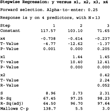
Figure 10.8 Forward selection results from Minitab for the Hald cement data.

From Table 10.3, we see that the regressor most highly correlated with y is x₄ (r_4y = −0.821), and since the t statistic associated with the model using x₄ is t = 4.77 and t_0.25/2,11 = 1.21, x₄ is added to the equation. At step 2 the regressor having the largest partial correlation with y (or the largest t statistic given that x₄ is in the model) is x₁, and since the partial F statistic for this regressor is t = 10.40, which exceeds t_0.25/2,10 = 1.22, x₁ is added to the model. In the third step, x₂ exhibits the highest partial correlation with y. The t statistic associated with this variable is 2.24, which is larger than t_0.25/2,9 = 1.23, and so x₂ is added to the model. At this point the only remaining candidate regressor is x₃, for which the t statistic does not exceed the cutoff value t_0.25/2,8 = 1.24, so the forward selection procedure terminates with

as the final model.

Backward Elimination Forward selection begins with no regressors in the model and attempts to insert variables until a suitable model is obtained. Backward elimination attempts to find a good model by working in the opposite direction. That is, we begin with a model that includes all K candidate regressors. Then the partial F statistic (or equivalently, a t statistic) is computed for each regressor as if it were the last variable to enter the model. The smallest of these partial F (or t) statistics is compared with a preselected value, F_OUT (or t_OUT), for example, and if the smallest partial F (or t), value is less than F_OUT (or t_OUT), that regressor is removed from the model. Now a regression model with K − 1 regressors is fit, the partial F (or t) statistics for this new model calculated, and the procedure repeated. The backward elimination algorithm terminates when the smallest partial F (or t) value is not less than the preselected cutoff value F_OUT (or t_OUT).

Backward elimination is often a very good variable selection procedure. It is particularly favored by analysts who like to see the effect of including all the candidate regressors, just so that nothing “obvious” will be missed.

Example 10.3 Backward Elimination—Hald Cement Data

We will illustrate backward elimination using the Hald cement data from Example 10.1. Figure 10.9 presents the results of using the Minitab version of backward elimination on those data. In this run we have selected the cutoff value by using α = 0.10, the default in Minitab. Minitab uses the t statistic for removing variables; thus, a regressor is dropped if the absolute value of its t statistic is less than t_OUT = t_0.1/2,n−p. Step 1 shows the results of fitting the full model. The smallest t value is 0.14, and it is associated with x₃. Thus, since t = 0.14 < t_OUT = t_0.10/2,8 = 1.86, x₃ is removed from the model. At step 2 in Figure 10.9, we see the results of fitting the three-variable model involving (x₁, x₂, x₄). The smallest t_statistic in this model, t = −1.37, is associated with x₄. Since |t| = 1.37 < t_OUT = t_0.20/2,9 = 1.83, x₄ is removed from the model. At step 3, we see the results of fitting the two-variable model involving (x₁, x₂). The smallest t statistic in this model is 12.41, associated with x₁, and since this exceeds t_OUT = t_0.10/2,10 = 1.81, no further regressors can be removed from the model. Therefore, backward elimination terminates, yielding the final model

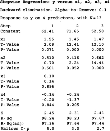
Figure 10.9 Backward selection results from Minitab for the Hald cement data.

Note that this is a different model from that found by forward selection. Furthermore, it is the model tentatively identified as best by the all-possible-regressions procedure.

Stepwise Regression The two procedures described above suggest a number of possible combinations. One of the most popular is the stepwise regression algorithm of Efroymson [1960]. Stepwise regression is a modification of forward selection in which at each step all regressors entered into the model previously are reassessed via their partial F (or t) statistics. A regressor added at an earlier step may now be redundant because of the relationships between it and regressors now in the equation. If the partial F (or t) statistic for a variable is less than F_OUT (or t_OUT), that variable is dropped from the model.

Stepwise regression requires two cutoff values, one for entering variables and one for removing them. Some analysts prefer to choose F_IN (or t_IN) = F_OUT (or t_OUT), although this is not necessary. Frequently we choose F_IN (or t_IN) > F_OUT (or t_OUT), making it relatively more difficult to add a regressor than to delete one.

Example 10.4 Stepwise Regression—Hald Cement Data

Figure 10.10 presents the results of using the Minitab stepwise regression algorithm on the Hald cement data. We have specified the α level for either adding or removing a regressor as 0.15. At step 1, the procedure begins with no variables in the model and tries to add x₄. Since the t statistic at this step exceeds t_IN = t_0.15/2,11 = 1.55, x₄ is added to the model. At step 2, x₁ is added to the model. If the t statistic value for x₄ is less than t_OUT = t_0.15/2,10 = 1.56, x₄ would be deleted. However, the t value for x₄ at step 2 is −12.62, so x₄ is retained. In step 3, the stepwise regression algorithm adds x₂ to the model. Then the t statistics for x₁ and x₄ are compared to t_OUT = t_0.15/2,9 = 1.57. Since for x₄ we find a t value of −1.37, and since |t| = 1.37 is less than t_OUT = 1.57, x₄ is deleted. Step 4 shows the results of removing x₄ from the model. At this point the only remaining candidate regressor is x₃, which cannot be added because its t value does not exceed t_IN. Therefore, stepwise regression terminates with the model

This is the same equation identified by the all-possible-regressions and backward elimination procedures.

Figure 10.10 Stepwise selection results from Minitab for the Hald cement data.

General Comments on Stepwise-Type Procedures The stepwise regression algorithms described above have been criticized on various grounds, the most common being that none of the procedures generally guarantees that the best subset regression model of any size will be identified. Furthermore, since all the stepwise-type procedures terminate with one final equation, inexperienced analysts may conclude that they have found a model that is in some sense optimal. Part of the problem is that it is likely, not that there is one best subset model, but that there are several equally good ones.

The analyst should also keep in mind that the order in which the regressors enter or leave the model does not necessarily imply an order of importance to the regressors. It is not unusual to find that a regressor inserted into the model early in the procedure becomes negligible at a subsequent step. This is evident in the Hald cement data, for which forward selection chooses x₄ as the first regressor to enter. However, when x₂ is added at a subsequent step, x₄ is no longer required because of the high intercorrelation between x₂ and x₄. This is in fact a general problem with the forward selection procedure. Once a regressor has been added, it cannot be removed at a later step.

Note that forward selection, backward elimination, and stepwise regression do not necessarily lead to the same choice of final model. The intercorrelation between the regressors affects the order of entry and removal. For example, using the Hald cement data, we found that the regressors selected by each procedure were as follows:

Some users have recommended that all the procedures be applied in the hopes of either seeing some agreement or learning something about the structure of the data that might be overlooked by using only one selection procedure. Furthermore, there is not necessarily any agreement between any of the stepwise-type procedures and all possible regressions. However, Berk [1978] has noted that forward selection tends to agree with all possible regressions for small subset sizes but not for large ones, while backward elimination tends to agree with all possible regressions for large subset sizes but not for small ones.

For these reasons stepwise-type variable selection procedures should be used with caution. Our own preference is for the stepwise regression algorithm followed by backward elimination. The backward elimination algorithm is often less adversely affected by the correlative structure of the regressors than is forward selection (see Mantel [1970]).

Stopping Rules for Stepwise Procedures Choosing the cutoff values F_IN (or t_IN) and/or F_OUT (or t_OUT) in stepwise-type procedures can be thought of as specifying a stopping rule for these algorithms. Some computer programs allow the analyst to specify these numbers directly, while others require the choice of a type 1 error rate α to generate the cutoff values. However, because the partial F (or t) value examined at each stage is the maximum of several correlated partial F (or t) variables, thinking of α as a level of significance or type 1 error rate is misleading. Several authors (e.g., Draper, Guttman, and Kanemasa [1971] and Pope and Webster [1972]) have investigated this problem, and little progress has been made toward either finding conditions under which the “advertised” level of significance on the t or F statistic is meaningful or developing the exact distribution of the F (or t)-to-enter and F (or t)-to-remove statistics.

Some users prefer to choose relatively small values of F_IN and F_OUT (or the equivalent t statistics) so that several additional regressors that would ordinarily be rejected by more conservative F values may be investigated. In the extreme we may choose F_IN and F_OUT so that all regressors are entered by forward selection or removed by backward elimination revealing one subset model of each size for p = 2, 3, …, K + 1. These subset models may then be evaluated by criteria such as C_p or MS_Res to determine the final model. We do not recommend this extreme strategy because the analyst may think that the subsets so determined are in some sense optimal when it is likely that the best subset model was overlooked. A very popular procedure is to set F_IN = F_OUT = 4, as this corresponds roughly to the upper 5% point of the F distribution. Still another possibility is to make several runs using different values for the cutoffs and observe the effect of the choice of criteria on the subsets obtained.

There have been several studies directed toward providing practical guidelines in the choice of stopping rules. Bendel and Afifi [1974] recommend α = 0.25 for forward selection. These are the defaults in Minitab. This would typically result in a numerical value of F_IN of between 1.3 and 2. Kennedy and Bancroft [1971] also suggest α = 0.25 for forward selection and recommend α = 0.10 for backward elimination. The choice of values for the cutoffs is largely a matter of the personal preference of the analyst, and considerable latitude is often taken in this area.

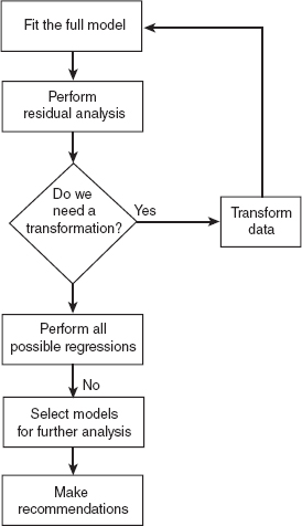
Figure 10.11 Flowchart of the model-building process.

10.3 STRATEGY FOR VARIABLE SELECTION AND MODEL BUILDING

Figure 10.11 summarizes a basic approach for variable selection and model building. The basic steps are as follows:

1. Fit the largest model possible to the data.
2. Perform a thorough analysis of this model.
3. Determine if a transformation of the response or of some of the regressors is necessary.
4. Determine if all possible regressions are feasible.
   • If all possible regressions are feasible, perform all possible regressions using such criteria as Mallow's C_p adjusted R², and the PRESS statistic to rank the best subset models.
   • If all possible regressions are not feasible, use stepwise selection techniques to generate the largest model such that all possible regressions are feasible. Perform all possible regressions as outlined above.
5. Compare and contrast the best models recommended by each criterion.
6. Perform a thorough analysis of the “best” models (usually three to five models).
7. Explore the need for further transformations.
8. Discuss with the subject-matter experts the relative advantages and disadvantages of the final set of models.

By now, we believe that the reader has a good idea of how to perform a thorough analysis of the full model. The primary reason for analyzing the full model is to get some idea of the “big picture.” Important questions include the following:

• What regressors seem important?
• Are there possible outliers?
• Is there a need to transform the response?
• Do any of the regressors need transformations?

It is crucial for the analyst to recognize that there are two basic reasons why one may need a transformation of the response:

• The analyst is using the wrong “scale” for the purpose. A prime example of this situation is gas mileage data. Most people find it easier to interpret the response as “miles per gallon”; however, the data are actually measured as “gallons per mile.” For many engineering data, the proper scale involves a log transformation.
• There are significant outliers in the data, especially with regard to the fit by the full model. Outliers represent failures by the model to explain some of the responses. In some cases, the responses themselves are the problem, for example, when they are mismeasured at the time of data collection. In other cases, it is the model itself that creates the outlier. In these cases, dropping one of the unimportant regressors can actually clear up this problem.

We recommend the use of all possible regressions to identify subset models whenever it is feasible. With current computing power, all possible regressions is typically feasible for 20–30 candidate regressors, depending on the total size of the data set. It is important to keep in mind that all possible regressions suggests the best models purely in terms of whatever criteria the analyst chooses to use. Fortunately, there are several good criteria available, especially Mallow's C_p, adjusted R², and the PRESS statistic. In general, the PRESS statistic tends to recommend smaller models than Mallow's C_p, which in turn tends to recommend smaller models than the adjusted R². The analyst needs to reflect on the differences in the models in light of each criterion used. All possible regressions inherently leads to the recommendation of several candidate models, which better allows the subject-matter expert to bring his or her knowledge to bear on the problem. Unfortunately, not all statistical software packages support the all-possible-regressions approach.

The stepwise methods are fast, easy to implement, and readily available in many software packages. Unfortunately, these methods do not recommend subset models that are necessarily best with respect to any standard criterion. Furthermore, these methods, by their very nature, recommend a single, final equation that the unsophisticated user may incorrectly conclude is in some sense optimal.

We recommend a two-stage strategy when the number of candidate regressors is too large to employ the all-possible-regressions approach initially. The first stage uses stepwise methods to “screen” the candidate regressors, eliminating those that clearly have negligible effects. We then recommend using the all-possible-regressions approach to the reduced set of candidate regressors. The analyst should always use knowledge of the problem environment and common sense in evaluating candidate regressors. When confronted with a large list of candidate regressors, it is usually profitable to invest in some serious thinking before resorting to the computer. Often, we find that we can eliminate some regressors on the basis of logic or engineering sense.

A proper application of the all-possible-regressions approach should produce several (three to five) final candidate models. At this point, it is critical to perform thorough residual and other diagnostic analyses of each of these final models. In making the final evaluation of these models, we strongly suggest that the analyst ask the following questions:

1. Are the usual diagnostic checks for model adequacy satisfactory? For example, do the residual plots indicate unexplained structure or outliers or are there one or more high leverage points that may be controlling the fit? Do these plots suggest other possible transformation of the response or of some of the regressors?
2. Which equations appear most reasonable? Do the regressors in the best model make sense in light of the problem environment? Which models make the most sense from the subject-matter theory?
3. Which models are most usable for the intended purpose? For example, a model intended for prediction that contains a regressor that is unobservable at the time the prediction needs to be made is unusable. Another example is a model that includes a regressor whose cost of collecting is prohibitive.
4. Are the regression coefficients reasonable? In particular, are the signs and magnitudes of the coefficients realistic and the standard errors relatively small?
5. Is there still a problem with multicollinearity?

If these four questions are taken seriously and the answers strictly applied, in some (perhaps many) instances there will be no final satisfactory regression equation. For example, variable selection methods do not guarantee correcting all problems with multicollinearity and influence. Often, they do; however, there are situations where highly related regressors still make significant contributions to the model even though they are related. There are certain data points that always seem to be problematic.

The analyst needs to evaluate all the trade-offs in making recommendations about the final model. Clearly, judgment and experience in the model's intended operation environment must guide the analyst as he/she makes decisions about the final recommended model.

Finally, some models that fit the data upon which they were developed very well may not predict new observations well. We recommend that the analyst assess the predictive ability of models by observing their performance on new data not used to build the model. If new data are not readily available, then the analyst should set aside some of the originally collected data (if practical) for this purpose. We discuss these issues in more detail in Chapter 11.

10.4 CASE STUDY: GORMAN AND TOMAN ASPHALT DATA USING SAS

Gorman and Toman (1966) present data concerning the rut depth of 31 asphalt pavements prepared under different conditions specified by five regressors. A sixth regressor is used as an indicator variable to separate the data into two sets of runs. The variables are as follows: y is the rut depth per million wheel passes, x₁ is the viscosity of the asphalt, x₂ is the percentage of asphalt in the surface course, x₃ is the percentage of asphalt in the base course, x₄ is the run, x₅ is the percentage of fines in the surface course, and x₆ is the percentage of voids in the surface course. It was decided to use the log of the viscosity as the regressor, instead of the actual viscosity, based upon consultation with a civil engineer familiar with this material. Viscosity is an example of a measurement that is usually more nearly linear when expressed on a log scale.

The run regressor is actually an indicator variable. In regression model building, indicator variables can often present unique challenges. In many cases the relationships between the response and the other regressors change depending on the specific level of the indicator. Readers familiar with experimental design will recognize the concept of interaction between the indicator variable and at least some of the other regressors. This interaction complicates the model-building process, the interpretation of the model, and the prediction of new (future) observations. In some cases, the variance of the response is very different at the different levels of the indicator variable, which further complicates model building and prediction.

An example helps us to see the possible complications brought about by an indicator variable. Consider a multinational wine-making firm that makes Cabernet Sauvignon in Australia, California, and France. This company wishes to model the quality of the wine as measured by its professional tasting staff according to the standard 100-point scale. Clearly, local soil and microclimate as well as the processing variables impact the taste of the wine. Some potential regressors, such as the age of the oak barrels used to age the wine, may behave similarly from region to region. Other possible regressors, such as the yeast used in the fermentation process, may behave radically differently across the regions. Consequently, there may be considerable variability in the ratings for the wines made from the three regions, and it may be quite difficult to find a single regression model that describes wine quality incorporating the indicator variables to model the three regions. This model would also be of minimal value in predicting wine quality for a Cabernet Sauvignon produced from grapes grown in Oregon. In some cases, the best thing to do is to build separate models for each level of the indicator variable.

TABLE 10.5 Gorman and Toman Asphalt Data

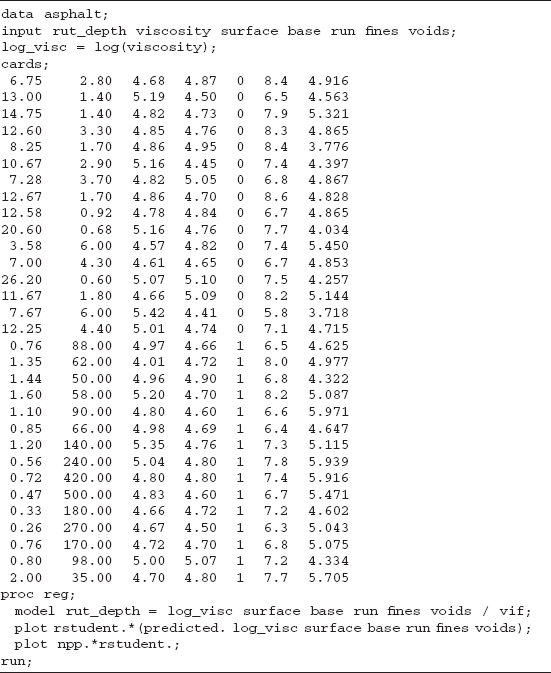
Table 10.5 gives the asphalt data. Table 10.6 gives the appropriate SAS code to perform the initial analysis of the data. Table 10.7 gives the resulting SAS output. Figures 10.12–10.19 give the residual plots from Minitab.

We note that the overall F test indicates that at least one regressor is important. The R² is 0.8060, which is good. The t tests on the individual coefficients indicate that only the log of the viscosity is important, which we will see later is misleading. The variance inflation factors indicate problems with log-visc and run. Figure 10.13 is the plot of the residuals versus the predicted values and indicates a major problem. This plot is consistant with the need for a log transformation of the response. We see a similar problem with Figure 10.14, which is the plot of the residuals versus the log of the viscosity. This plot is also interesting because it suggests that there may be two distinct models: one for the low viscosity and another for the high viscosity. This point is reemphasized in Figure 10.17, which is the residuals versus run plot. It looks like the first run (run 0) involved all the low-viscosity material while the second run (run 1) involved the high-viscosity material.

TABLE 10.6 Initial SAS Code for Untransformed Response

The plot of residuals versus run reveals a distinct difference in the variability between these two runs. We leave the exploration of this issue as an exercise. The residual plots also indicate one possible outlier.

TABLE 10.7 SAS Output for Initial Analysis of Asphalt Data

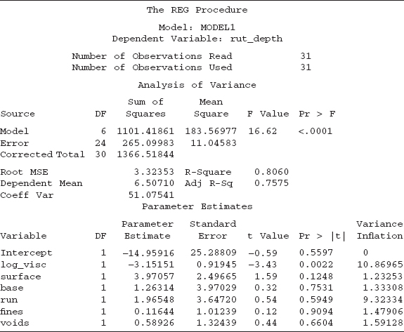
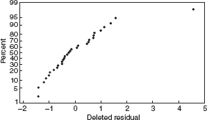
Figure 10.12 Normal probability plot of the residuals for the asphalt data.

Figure 10.13 Residuals versus the fitted values for the asphalt data.

Figure 10.14 Residuals versus the log of the viscosity for the asphalt data.

Figure 10.15 Residuals versus surface for the asphalt data.

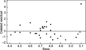
Figure 10.16 Residuals versus base for the asphalt data.

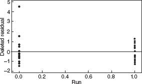
Figure 10.17 Residuals versus run for the asphalt data.

Figure 10.18 Residuals versus fines for the asphalt data.

Figure 10.19 Residuals versus voids for the asphalt data.

TABLE 10.8 SAS Code for Analyzing Transformed Response Using Full Model

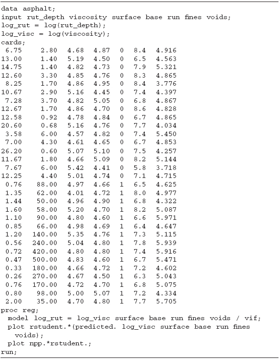
Table 10.8 gives the SAS code to generate the analysis on the log of the rut depth data. Table 10.9 gives the resulting SAS output.

Once again, the overall F test indicates that at least one regressor is important. The R² is very good. It is important to note that we cannot directly compare the R² from the untransformed response to the R² of the transformed response. However, the observed improvement in this case does support the use of the transformation. The t tests on the individual coefficients continue to suggest that the log of the viscosity is important. In addition, surface also looks important. The regressor voids appear marginal. There are no changes in the variance inflation factors because we only transformed the response, the variance inflation factors depend only on the relationships among the regressors.

TABLE 10.9 SAS Output for Transformed Response and Full Model

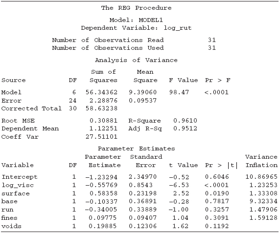
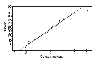
Figure 10.20 Normal probability plot of the residuals for the asphalt data after the log transformation.

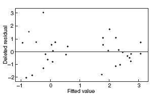
Figure 10.21 Residuals versus the fitted values for the asphalt data after the log transformation.

Figure 10.22 Residuals versus the log of the viscosity for the asphalt data after the log transformation.

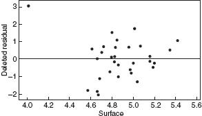
Figure 10.23 Residuals versus surface for the asphalt data after the log transformation.

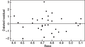
Figure 10.24 Residuals versus base for the asphalt data after the log transformation.

Figure 10.25 Residuals versus run for the asphalt data after the log transformation.

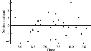
Figure 10.26 Residuals versus fines for the asphalt data after the log transformation.

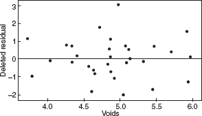
Figure 10.27 Residuals versus voids for the asphalt data after the log transformation.

Figures 10.20–10.27 give the residual plots. The plots of residual versus predicted value and residual versus individual regressor look much better, again supporting the value of the transformation. Interestingly, the normal probability plot of the residuals actually looks a little worse. On the whole, we should feel comfortable using the log of the rut depth as the response. We shall restrict all further analysis to the transformed response.

TABLE 10.10 SAS Code for All Possible Regressions of Asphalt Data

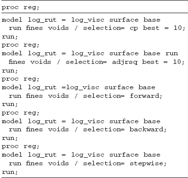
Table 10.10 gives the SAS source code for the all-possible-regressions approach. Table 10.11 gives the annotated output.

Both the stepwise and backward selection techniques suggested the variables log of viscosity, surface, and voids. The forward selection techniques suggested the variables log of viscosity, surface, voids, run, and fines. Both of these models were in the top five models in terms of the C_p statistic.

We can obtain the PRESS statistic for a specific model by the following SAS model statement:

model log_rut=log_visc surface voids/p clm cli;

Table 10.12 summarizes the C_p, adjusted R², and PRESS information for the best five models in terms of the C_p statistics. This table represents one of the very rare situations where a single model seems to dominate.

Table 10.13 gives the SAS code for analyzing the model that regresses log of rut depth against log of viscosity, surface, and voids. Table 10.14 gives the resulting SAS output. The overall F test is very strong. The R² is 0.9579, which is quite high. All three of the regressors are important. We see no problems with multicollinearity as evidenced by the variance inflation factors. The residual plots, which we do not show, all look good. Observation 18 has the largest hat diagonal, R-student, and DFFITS value, which indicates that it is influential. The DFBETAS suggest that this observation impacts the intercept and the surface regressor. On the whole, we should feel comfortable recommending this model.

TABLE 10.11 Annotated SAS Output for All Possible Regressions of Asphalt Data

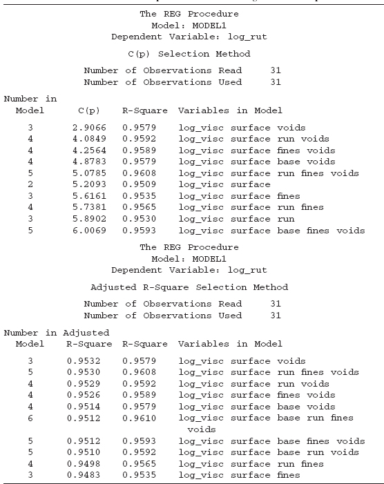
TABLE 10.12 Summary of the Best Models for Asphalt Data

TABLE 10.13 SAS Code for Recommended Model for Asphalt Data

TABLE 10.14 SAS Output for Analysis of Recommended Model

PROBLEMS

10.1 Consider the National Football League data in Table B.1.

1. Use the forward selection algorithm to select a subset regression model.
2. Use the backward elimination algorithm to select a subset regression model.
3. Use stepwise regression to select a subset regression model.
4. Comment on the final model chosen by these three procedures.

10.2 Consider the National Football League data in Table B.1. Restricting your attention to regressors x₁ (rushing yards), x₂ (passing yards), x₄ (field goal percentage), x₇ (percent rushing), x₈ (opponents' rushing yards), and x₉ (opponents' passing yards), apply the all-possible-regressions procedure. Evaluate R²_p, C_p, and MS_Res for each model. Which subset of regressors do you recommend?.

10.3 In stepwise regression, we specify that F_IN ≥ F_OUT (or t_IN ≥ t_OUT). Justify this choice of cutoff values.

10.4 Consider the solar thermal energy test data in Table B.2.

1. Use forward selection to specify a subset regression model.
2. Use backward elimination to specify a subset regression model.
3. Use stepwise regression to specify a subset regression model.
4. Apply all possible regressions to the data. Evaluate R²_p, C_p, and MS_Res for each model. Which subset model do you recommend?
5. Compare and contrast the models produced by the variable selection strategies in parts a–d.

10.5 Consider the gasoline mileage performance data in Table B.3.

1. Use the all-possible-regressions approach to find an appropriate regression model.
2. Use stepwise regression to specify a subset regression model. Does this lead to the same model found in part a?

10.6 Consider the property valuation data found in Table B.4.

1. Use the all-possible-regressions method to find the “best” set of regressors.
2. Use stepwise regression to select a subset regression model. Does this model agree with the one found in part a?

10.7 Use stepwise regression with F_IN = F_OUT = 4.0 to find the “best” set of regressor variables for the Belle Ayr liquefaction data in Table B.5. Repeat the analysis with F_IN = F_OUT = 2.0. Are there any substantial differences in the models obtained?.

10.8 Use the all-possible-regressions method to select a subset regression model for the Belle Ayr liquefaction data in Table B.5. Evaluate the subset models using the C_p criterion. Justify your choice of final model using the standard checks for model adequacy.

10.9 Analyze the tube-flow reactor data in Table B.6 using all possible regressions. Evaluate the subset models using the R²_p, C_p, and MS_Res criteria. Justify your choice of final model using the standard checks for model adequacy.

10.10 Analyze the air pollution and mortality data in Table B.15 using all possible regressions. Evaluate the subset models using the R²_p, C_p, and MS_Res criteria. Justify your choice of the final model using the standard checks for model adequacy.

1. Use the all-possible-regressions approach to find the best subset model for rut depth. Use C_p as the criterion.
2. Repeat part a using MS_Res as the criterion. Did you find the same model?
3. Use stepwise regression to find the best subset model. Did you find the same equation that you found in either part a or b above?

10.11 Consider the all-possible-regressions analysis of Hald's cement data in Example 10.1. If the objective is to develop a model to predict new observations, which equation would you recommend and why?

10.12 Consider the all-possible-regressions analysis of the National Football League data in Problem 10.2. Identify the subset regression models that are R² adequate (0.05).

10.13 Suppose that the full model is y_i = β₀ + β₁x_i1 + β₂x_i2 + ε_ii = 1, 2, …, n, where x_i1 and x_i2 have been coded so that S₁₁ = S₂₂ = 1. We will also consider fitting a subset model, say y_i = β₀ + β₁x_i1 + ε_i.

1. Let be the least-squares estimate of β₁ from the full model. Show that , where r₁₂ is the correlation between x₁ and x₂.
2. Let be the least-squares estimate of β₁ from the subset model. Show that . Is β₁ estimated more precisely from the subset model or from the full model?
3. Show that . Under what circumstances is an unbiased estimator of β₁?
4. Find the mean square error for the subset estimator . Compare with . Under what circumstances is a preferable estimator, with respect to MSE?

You may find it helpful to reread Section 10.1.2.

10.14 Table B.11 presents data on the quality of Pinot Noir wine.

1. Build an appropriate regression model for quality y using the all-possible-regressions approach. Use C_p as the model selection criterion, and incorporate the region information by using indicator variables.
2. For the best two models in terms of C_p, investigate model adequacy by using residual plots. Is there any practical basis for selecting between these models?
3. Is there any difference between the two models in part b in terms of the PRESS statistic?

10.15 Use the wine quality data in Table B.11 to construct a regression model for quality using the stepwise regression approach. Compare this model to the one you found in Problem 10.4, part a.

10.16 Rework Problem 10.14, part a, but exclude the region information.

1. Comment on the difference in the models you have found. Is there indication that the region information substantially improves the model?
2. Calculate confidence intervals as mean quality for all points in the data set using the models from part a of this problem and Problem 10.14, part a. Based on this analysis, which model would you prefer?

10.17 Table B.12 presents data on a heat treating process used to carburize gears. The thickness of the carburized layer is a critical factor in overall reliability of this component. The response variable y = PITCH is the result of a carbon analysis on the gear pitch for a cross-sectioned part. Use all possible regressions and the C_p criterion to find an appropriate regression model for these data. Investigate model adequacy using residual plots.

10.18 Reconsider the heat treating data from Table B.12. Fit a model to the PITCH response using the variables

as regressors. How does this model compare to the one you found by the all-possible-regressions approach of Problem 10.17?

10.19 Repeat Problem 10.17 using the two cross-product variables defined in Problem 10.18 as additional candidate regressors. Comment on the model that you find.

10.20 Compare the models that you have found in Problems 10.17, 10.18, and 10.19 by calculating the confidence intervals on the mean of the response PITCH for all points in the original data set. Based on a comparison of these confidence intervals, which model would you prefer? Now calculate the PRESS statistic for these models. Which model would PRESS indicate is likely to be the best for predicting new observations on PITCH?.

10.21 Table B.13 presents data on the thrust of a jet turbine engine and six candidate regressors. Use all possible regressions and the C_p criterion to find an appropriate regression model for these data. Investigate model adequacy using residual plots.

10.22 Reconsider the jet turbine engine thrust data in Table B.13. Use stepwise regression to find an appropriate regression model for these data. Investigate model adequacy using residual plots. Compare this model with the one found by the all-possible-regressions approach in Problem 10.21.

10.23 Compare the two best models that you have found in Problem 10.21 in terms of C_p by calculating the confidence intervals on the mean of the thrust response for all points in the original data set. Based on a comparison of these confidence intervals, which model would you prefer? Now calculate the PRESS statistic for these models. Which model would PRESS indicate is likely to be the best for predicting new observations on thrust?

10.24 Table B.14 presents data on the transient points of an electronic inverter. Use all possible regressions and the C_p criterion to find an appropriate regression model for these data. Investigate model adequacy using residual plots.

10.25 Reconsider the electronic inverter data in Table B.14. Use stepwise regression to find an appropriate regression model for these data. Investigate model adequacy using residual plots. Compare this model with the one found by the all-possible-regressions approach in Problem 10.24.

10.26 Compare the two best models that you have found in Problem 10.24 in terms of C_p by calculating the confidence intervals on the mean of the response for all points in the original data set. Based on a comparison of these confidence intervals, which model would you prefer? Now calculate the PRESS statistic for these models. Which model would PRESS indicate is likely to be the best for predicting new response observations?

10.27 Reconsider the electronic inverter data in Table B.14. In Problems 10.24 and 10.25, you built regression models for the data using different variable selection algorithms. Suppose that you now learn that the second observation was incorrectly recorded and should be ignored.

1. Fit a model to the modified data using all possible regressions, using C_p as the criterion. Compare this model to the model you found in Problem 10.24.
2. Use stepwise regression to find an appropriate model for the modified data. Compare this model to the one you found in Problem 10.25.
3. Calculate the confidence intervals as the mean response for all points in the modified data set. Compare these results with the confidence intervals from Problem 10.26. Discuss your findings.

10.28 Consider the electronic inverter data in Table B.14. Delete observation 2 from the original data. Electrical engineering theory suggests that we should define new variables as follows: y* = ln y, , and .

1. Find an appropriate subset regression model for these data using all possible regressions and the C_p criterion.
2. Plot the residuals versus for this model. Comment on the plots.
3. Discuss how you could compare this model to the ones built using the original response and regressors in Problem 10.27.

10.29 Consider the Gorman and Toman asphalt data analyzed in Section 10.4. Recall that run is an indicator variable.

1. Perform separate analyses of those data for run = 0 and run = 1.
2. Compare and contrast the results of the two analyses from part a.
3. Compare and contrast the results of the two analyses from part a with the results of the analysis from Section 10.4.

10.30 Table B.15 presents data on air pollution and mortality. Use the all-possible-regressions selection on the air pollution data to find appropriate models for these data. Perform a thorough analysis of the best candidate models. Compare your results with stepwise regression. Thoroughly discuss your recommendations.

10.31 Use the all-possible-regressions selection on the patient satisfaction data in Table B.17. Perform a thorough analysis of the best candidate models. Compare your results with stepwise regression. Thoroughly discuss your recommendations.

10.32 Use the all-possible-regressions selection on the fuel consumption data in Table B.18. Perform a thorough analysis of the best candidate models. Compare your results with stepwise regression. Thoroughly discuss your recommendations.

10.33 Use the all-possible-regressions selection on the wine quality of young red wines data in Table B.19. Perform a thorough analysis of the best candidate models. Compare your results with stepwise regression. Thoroughly discuss your recommendations.

10.34 Use the all-possible-regressions selection on the methanol oxidation data in Table B.20. Perform a thorough analysis of the best candidate models. Compare your results with stepwise regression. Thoroughly discuss your recommendations.