CHAPTER 1

INTRODUCTION

1.1 REGRESSION AND MODEL BUILDING

Regression analysis is a statistical technique for investigating and modeling the relationship between variables. Applications of regression are numerous and occur in almost every field, including engineering, the physical and chemical sciences, economics, management, life and biological sciences, and the social sciences. In fact, regression analysis may be the most widely used statistical technique.

As an example of a problem in which regression analysis may be helpful, suppose that an industrial engineer employed by a soft drink beverage bottler is analyzing the product delivery and service operations for vending machines. He suspects that the time required by a route deliveryman to load and service a machine is related to the number of cases of product delivered. The engineer visits 25 randomly chosen retail outlets having vending machines, and the in-outlet delivery time (in minutes) and the volume of product delivered (in cases) are observed for each. The 25 observations are plotted in Figure 1.1a. This graph is called a scatter diagram. This display clearly suggests a relationship between delivery time and delivery volume; in fact, the impression is that the data points generally, but not exactly, fall along a straight line. Figure 1.1b illustrates this straight-line relationship.

If we let y represent delivery time and x represent delivery volume, then the equation of a straight line relating these two variables is

where β₀ is the intercept and β₁ is the slope. Now the data points do not fall exactly on a straight line, so Eq. (1.1) should be modified to account for this. Let the difference between the observed value of y and the straight line (β₀ + β₁x) be an error ε. It is convenient to think of ε as a statistical error; that is, it is a random variable that accounts for the failure of the model to fit the data exactly. The error may be made up of the effects of other variables on delivery time, measurement errors, and so forth. Thus, a more plausible model for the delivery time data is

Figure 1.1 (a) Scatter diagram for delivery volume. (b) Straight-line relationship between delivery time and delivery volume.

Equation (1.2) is called a linear regression model. Customarily x is called the independent variable and y is called the dependent variable. However, this often causes confusion with the concept of statistical independence, so we refer to x as the predictor or regressor variable and y as the response variable. Because Eq. (1.2) involves only one regressor variable, it is called a simple linear regression model.

To gain some additional insight into the linear regression model, suppose that we can fix the value of the regressor variable x and observe the corresponding value of the response y. Now if x is fixed, the random component ε on the right-hand side of Eq. (1.2) determines the properties of y. Suppose that the mean and variance of ε are 0 and σ². respectively. Then the mean response at any value of the regressor variable is

Notice that this is the same relationship that we initially wrote down following inspection of the scatter diagram in Figure 1.1a. The variance of y given any value of x is

Thus, the true regression model μ_x|y = β₀ + β₁x isa line of mean values, that is, the height of the regression line at any value of x is just the expected value of y for that x. The slope, β₁ can be interpreted as the change in the mean of y for a unit change in x. Furthermore, the variability of y at a particular value of x is determined by the variance of the error component of the model, a². This implies that there is a distribution of y values at each x and that the variance of this distribution is the same at each x.

Figure 1.2 How observations are generated in linear regression.

Figure 1.3 Linear regression approximation of a complex relationship.

For example, suppose that the true regression model relating delivery time to delivery volume is μ_y|x = 3.5 + 2x, and suppose that the variance is σ² = 2. Figure 1.2 illustrates this situation. Notice that we have used a normal distribution to describe the random variation in ε. Since y is the sum of a constant β₀ + β₁x (the mean) and a normally distributed random variable, y is a normally distributed random variable. For example, if x = 10 cases, then delivery time y has a normal distribution with mean 3.5 + 2(10) = 23.5 minutes and variance 2. The variance σ² determines the amount of variability or noise in the observations y on delivery time. When σ² is small, the observed values of delivery time will fall close to the line, and when σ² is large, the observed values of delivery time may deviate considerably from the line.

In almost all applications of regression, the regression equation is only an approximation to the true functional relationship between the variables of interest. These functional relationships are often based on physical, chemical, or other engineering or scientific theory, that is, knowledge of the underlying mechanism. Consequently, these types of models are often called mechanistic models. Regression models, on the other hand, are thought of as empirical models. Figure 1.3 illustrates a situation where the true relationship between y and x is relatively complex, yet it may be approximated quite well by a linear regression equation. Sometimes the underlying mechanism is more complex, resulting in the need for a more complex approximating function, as in Figure 1.4, where a “piecewise linear” regression function is used to approximate the true relationship between y and x.

Generally regression equations are valid only over the region of the regressor variables contained in the observed data. For example, consider Figure 1.5. Suppose that data on y and x were collected in the interval x₁ ≤ x ≤ x₂. Over this interval the linear regression equation shown in Figure 1.5 is a good approximation of the true relationship. However, suppose this equation were used to predict values of y for values of the regressor variable in the region x₂ ≤ x ≤ x₃. Clearly the linear regression model is not going to perform well over this range of x because of model error or equation error.

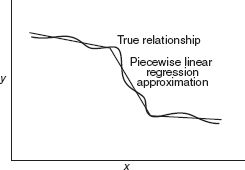
Figure 1.4 Piecewise linear approximation of a complex relationship.

Figure 1.5 The danger of extrapolation in regression.

In general, the response variable y may be related to k regressors, x₁, x₂,…, x_k, so that

This is called a multiple linear regression model because more than one regressor is involved. The adjective linear is employed to indicate that the model is linear in the parameters β₀, β₁,…,β_k, not because y isa linear function of the x's. We shall see subsequently that many models in which y is related to the x's in a nonlinear fashion can still be treated as linear regression models as long as the equation is linear in the β's.

An important objective of regression analysis is to estimate the unknown parameters in the regression model. This process is also called fitting the model to the data. We study several parameter estimation techniques in this book. One of these techmques is the method of least squares (introduced in Chapter 2). For example, the least-squares fit to the delivery time data is

where ŷ is the fitted or estimated value of delivery time corresponding to a delivery volume of x cases. This fitted equation is plotted in Figure 1.1b.

The next phase of a regression analysis is called model adequacy checking, in which the appropriateness of the model is studied and the quality of the fit ascertained. Through such analyses the usefulness of the regression model may be determined. The outcome of adequacy checking may indicate either that the model is reasonable or that the original fit must be modified. Thus, regression analysis is an iterative procedure, in which data lead to a model and a fit of the model to the data is produced. The quality of the fit is then investigated, leading either to modification of the model or the fit or to adoption of the model. This process is illustrated several times in subsequent chapters.

A regression model does not imply a cause-and-effect relationship between the variables. Even though a strong empirical relationship may exist between two or more variables, this cannot be considered evidence that the regressor variables and the response are related in a cause-and-effect manner. To establish causality, the relationship between the regressors and the response must have a basis outside the sample data—for example, the relationship may be suggested by theoretical considerations. Regression analysis can aid in confirming a cause-and-effect relationship, but it cannot be the sole basis of such a claim.

Finally it is important to remember that regression analysis is part of a broader data-analytic approach to problem solving. That is, the regression equation itself may not be the primary objective of the study. It is usually more important to gain insight and understanding concerning the system generating the data.

1.2 DATA COLLECTION

An essential aspect of regression analysis is data collection. Any regression analysis is only as good as the data on which it is based. Three basic methods for collecting data are as follows:

• A retrospective study based on historical data
• An observational study
• A designed experiment

A good data collection scheme can ensure a simplified and a generally more applicable model. A poor data collection scheme can result in serious problems for the analysis and its interpretation. The following example illustrates these three methods.

Example 1.1

Consider the acetone–butyl alcohol distillation column shown in Figure 1.6. The operating personnel are interested in the concentration of acetone in the distillate (product) stream. Factors that may influence this are the reboil temperature, the condensate temperature, and the reflux rate. For this column, operating personnel maintain and archive the following records:

• The concentration of acetone in a test sample taken every hour from the product stream
• The reboil temperature controller log, which is a plot of the reboil temperature
• The condenser temperature controller log
• The nominal reflux rate each hour

The nominal reflux rate is supposed to be constant for this process. Only infrequently does production change this rate. We now discuss how the three different data collection strategies listed above could be applied to this process.

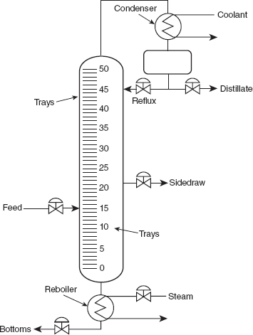
Figure 1.6 Acetone–butyl alcohol distillation column.

Retrospective Study We could pursue a retrospective study that would use either all or a sample of the historical process data over some period of time to determine the relationships among the two temperatures and the reflux rate on the acetone concentration in the product stream. In so doing, we take advantage of previously collected data and minimize the cost of the study. However, these are several problems:

1. We really cannot see the effect of reflux on the concentration since we must assume that it did not vary much over the historical period.
2. The data relating the two temperatures to the acetone concentration do not correspond directly. Constructing an approximate correspondence usually requires a great deal of effort.
3. Production controls temperatures as tightly as possible to specific target values through the use of automatic controllers. Since the two temperatures vary so little over time, we will have a great deal of difficulty seeing their real impact on the concentration.
4. Within the narrow ranges that they do vary, the condensate temperature tends to increase with the reboil temperature. As a result, we will have a great deal of difficulty separating out the individual effects of the two temperatures. This leads to the problem of collinearity or multicollinearity, which we discuss in Chapter 9.

Retrospective studies often offer limited amounts of useful information. In general, their primary disadvantages are as follows:

• Some of the relevant data often are missing.
• The reliability and quality of the data are often highly questionable.
• The nature of the data often may not allow us to address the problem at hand.
• The analyst often tries to use the data in ways they were never intended to be used.
• Logs, notebooks, and memories may not explain interesting phenomena identified by the data analysis.

Using historical data always involves the risk that, for whatever reason, some of the data were not recorded or were lost. Typically, historical data consist of information considered critical and of information that is convenient to collect. The convenient information is often collected with great care and accuracy. The essential information often is not. Consequently, historical data often suffer from transcription errors and other problems with data quality. These errors make historical data prone to outliers, or observations that are very different from the bulk of the data. A regression analysis is only as reliable as the data on which it is based.

Just because data are convenient to collect does not mean that these data are particularly useful. Often, data not considered essential for routine process monitoring and not convenient to collect do have a significant impact on the process. Historical data cannot provide this information since they were never collected. For example, the ambient temperature may impact the heat losses from our distillation column. On cold days, the column loses more heat to the environment than during very warm days. The production logs for this acetone–butyl alcohol column do not record the ambient temperature. As a result, historical data do not allow the analyst to include this factor in the analysis even though it may have some importance.

In some cases, we try to use data that were collected as surrogates for what we really needed to collect. The resulting analysis is informative only to the extent that these surrogates really reflect what they represent. For example, the nature of the inlet mixture of acetone and butyl alcohol can significantly affect the column's performance. The column was designed for the feed to be a saturated liquid (at the mixture's boiling point). The production logs record the feed temperature but do not record the specific concentrations of acetone and butyl alcohol in the feed stream. Those concentrations are too hard to obtain on a regular basis. In this case, inlet temperature is a surrogate for the nature of the inlet mixture. It is perfectly possible for the feed to be at the correct specific temperature and the inlet feed to be either a subcooled liquid or a mixture of liquid and vapor.

In some cases, the data collected most casually, and thus with the lowest quality, the least accuracy, and the least reliability, turn out to be very influential for explaining our response. This influence may be real, or it may be an artifact related to the inaccuracies in the data. Too many analyses reach invalid conclusions because they lend too much credence to data that were never meant to be used for the strict purposes of analysis.

Finally, the primary purpose of many analyses is to isolate the root causes underlying interesting phenomena. With historical data, these interesting phenomena may have occurred months or years before. Logs and notebooks often provide no significant insights into these root causes, and memories clearly begin to fade over time. Too often, analyses based on historical data identify interesting phenomena that go unexplained.

Observational Study We could use an observational study to collect data for this problem. As the name implies, an observational study simply observes the process or population. We interact or disturb the process only as much as is required to obtain relevant data. With proper planning, these studies can ensure accurate, complete, and reliable data. On the other hand, these studies often provide very limited information about specific relationships among the data.

In this example, we would set up a data collection form that would allow the production personnel to record the two temperatures and the actual reflux rate at specified times corresponding to the observed concentration of acetone in the product stream. The data collection form should provide the ability to add comments in order to record any interesting phenomena that may occur. Such a procedure would ensure accurate and reliable data collection and would take care of problems 1 and 2 above. This approach also minimizes the chances of observing an outlier related to some error in the data. Unfortunately, an observational study cannot address problems 3 and 4. As a result, observational studies can lend themselves to problems with collinearity.

Designed Experiment The best data collection strategy for this problem uses a designed experiment where we would manipulate the two temperatures and the reflux ratio, which we would call the factors, according to a well-defined strategy, called the experimental design. This strategy must ensure that we can separate out the effects on the acetone concentration related to each factor. In the process, we eliminate any collinearity problems. The specified values of the factors used in the experiment are called the levels. Typically, we use a small number of levels for each factor, such as two or three. For the distillation column example, suppose we use a “high” or +1 and a “low” or –1 level for each of the factors. We thus would use two levels for each of the three factors. A treatment combination is a specific combination of the levels of each factor. Each time we carry out a treatment combination is an experimental run or setting. The experimental design or plan consists of a series of runs.

For the distillation example, a very reasonable experimental strategy uses every possible treatment combination to form a basic experiment with eight different settings for the process. Table 1.1 presents these combinations of high and low levels.

Figure 1.7 illustrates that this design forms a cube in terms of these high and low levels. With each setting of the process conditions, we allow the column to reach equilibrium, take a sample of the product stream, and determine the acetone concentration. We then can draw specific inferences about the effect of these factors. Such an approach allows us to proactively study a population or process.

TABLE 1.1 Designed Experiment for the Distillation Column

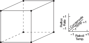
Figure 1.7 The designed experiment for the distillation column.

1.3 USES OF REGRESSION

Regression models are used for several purposes, including the following:

1. Data description
2. Parameter estimation
3. Prediction and estimation
4. Control

Engineers and scientists frequently use equations to summarize or describe a set of data. Regression analysis is helpful in developing such equations. For example, we may collect a considerable amount of delivery time and delivery volume data, and a regression model would probably be a much more convenient and useful summary of those data than a table or even a graph.

Sometimes parameter estimation problems can be solved by regression methods. For example, chemical engineers use the Michaelis–Menten equation y = β₁x/(x + β₂) + ε to describe the relationship between the velocity of reaction y and concentration x. Now in this model, β₁ is the asymptotic velocity of the reaction, that is, the maximum velocity as the concentration gets large. If a sample of observed values of velocity at different concentrations is available, then the engineer can use regression analysis to fit this model to the data, producing an estimate of the maximum velocity. We show how to fit regression models of this type in Chapter 12.

Many applications of regression involve prediction of the response variable. For example, we may wish to predict delivery time for a specified number of cases of soft drinks to be delivered. These predictions may be helpful in planning delivery activities such as routing and scheduling or in evaluating the productivity of delivery operations. The dangers of extrapolation when using a regression model for prediction because of model or equation error have been discussed previously (see Figure 1.5). However, even when the model form is correct, poor estimates of the model parameters may still cause poor prediction performance.

Regression models may be used for control purposes. For example, a chemical engineer could use regression analysis to develop a model relating the tensile strength of paper to the hardwood concentration in the pulp. This equation could then be used to control the strength to suitable values by varying the level of hardwood concentration. When a regression equation is used for control purposes, it is important that the variables be related in a causal manner. Note that a cause-and-effect relationship may not be necessary if the equation is to be used only for prediction. In this case it is only necessary that the relationships that existed in the original data used to build the regression equation are still valid. For example, the daily electricity consumption during August in Atlanta, Georgia, may be a good predictor for the maximum daily temperature in August. However, any attempt to reduce the maximum temperature by curtailing electricity consumption is clearly doomed to failure.

1.4 ROLE OF THE COMPUTER

Building a regression model is an iterative process. The model-building process is illustrated in Figure 1.8. It begins by using any theoretical knowledge of the process that is being studied and available data to specify an initial regression model. Graphical data displays are often very useful in specifying the initial model. Then the parameters of the model are estimated, typically by either least squares or maximum likelihood. These procedures are discussed extensively in the text. Then model adequacy must be evaluated. This consists of looking for potential misspecification of the model form, failure to include important variables, including unnecessary variables, or unusual/inappropriate data. If the model is inadequate, then must be made and the parameters estimated again. This process may be repeated several times until an adequate model is obtained. Finally, model validation should be carried out to ensure that the model will produce results that are acceptable in the final application.

A good regression computer program is a necessary tool in the model-building process. However, the routine application of standard regression compnter programs often does not lead to successful results. The computer is not a substitute for creative thinking about the problem. Regression analysis requires the intelligent and artful use of the computer. We must learn how to interpret what the computer is telling us and how to incorporate that information in subsequent models. Generally, regression computer programs are part of more general statistics software packages, such as Minitab, SAS, JMP, and R. We discuss and illustrate the use of these packages throughout the book. Appendix D contains details of the SAS procedures typically used in regression modeling along with basic instructions for their use. Appendix E provides a brief introduction to the R statistical software package. We present R code for doing analyses throughout the text. Without these skills, it is virtually impossible to successfully build a regression model.

Figure 1.8 Regression model-building process.