CHAPTER 3

MULTIPLE LINEAR REGRESSION

A regression model that involves more than one regressor variable is called a multiple regression model. Fitting and analyzing these models is discussed in this chapter. The results are extensions of those in Chapter 2 for simple linear regression.

3.1 MULTIPLE REGRESSION MODELS

Suppose that the yield in pounds of conversion in a chemical process depends on temperature and the catalyst concentration. A multiple regression model that might describe this relationship is

where y denotes the yield, x₁ denotes the temperature, and x₂ denotes the catalyst concentration. This is a multiple linear regression model with two regressor variables. The term linear is used because Eq. (3.1) is a linear function of the unknown parameters β₀, β₁ and β₂.

The regression model in Eq. (3.1) describes a plane in the three-dimensional space of y, x₁ and x₂. Figure 3.1a shows this regression plane for the model

where we have assumed that the expected value of the error term ε in Eq. (3.1) is zero. The parameter β₀ is the intercept of the regression plane. If the range of the data includes x₁ = x₂ = 0, then β₀ is the mean of y when x₁ = x₂ = 0. Otherwise β₀ has no physical interpretation. The parameter β₁ indicates the expected change in response(y) per unit change in x₁ when x₂ is held constant. Similarly β;₂ measures the expected change in y per unit change in x₁ when x₂ is held constant. Figure 3.1b shows a contour plot of the regression model, that is, lines of constant expected response E(y) as a function of x₁ and x₂. Notice that the contour lines in this plot are parallel straight lines.

Figure 3.1 (a) The regression plane for the model E(y) = 50 + 10x₁ + 7x₂. (b) The contour plot.

In general, the response y may be related to k regressor or predictor variables. The model

is called a mnltiple linear regression model with k regressors. The parameters β_j, j = 0, 1,…k, are called the regression coefficients. This model describes a hyperplane in the k-dimensional space of the regressor variables x_j. The parameter β_j represents the expected change in the response y per unit change in x_j when all of the remaining regressor variables x_i (i ≠ j) are held constant. For this reason the parameters β_j, j = 1,2,…,k, are often called partial regression coefficients.

Multiple linear regression models are often used as empirical models or approximating functions. That is, the true functional relationship between y and x₁, x₂,…,x_k is unknown, but over certain ranges of the regressor variables the linear regression model is an adequate approximation to the true unknown function.

Models that are more complex in structure than Eq. (3.2) may often still be analyzed by multiple linear regression techniques. For example, consider the cubic polynomial model

If we let x₁ = x, x₂ = x², and x₃ = x³, then Eq. (3.3) can be written as

which is a multiple linear regression model with three regressor variables. Polynomial models are discussed in more detail in Chapter 7.

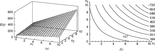
Figure 3.2 (a) Three-dimensional plot of regression model E(y) = 50 + 10x₁ + 7x₂ + 5x₁x₂. (b) The contour plot.

Models that include interaction effects may also be analyzed by multiple linear regression methods. For example, suppose that the model is

If we let x₃ = x₁x₂ and β₃ = β₁₂, then Eq. (3.5) can be written as

which is a linear regression model.

Figure 3.2a shows the three-dimensional plot of the regression model

and Figure 3.2b the corresponding two-dimensional contour plot. Notice that, although this model is a linear regression model, the shape of the surface that is generated by the model is not linear. In general, any regression model that is linear in the parameters (the β's) is a linear regression model, regardless of the shape of the surface that it generates.

Figure 3.2 provides a nice graphical interpretation of an interaction. Generally, interaction implies that the effect produced by changing one variable (x₁, say) depends on the level of the other variable (x₂). For example, Figure 3.2 shows that changing x₁ from 2 to 8 produces a much smaller change in E(y) when x₂ = 2 than when x₂ = 10. Interaction effects occur frequently in the study and analysis of real-world systems, and regression methods are one of the techniques that we can use to describe them.

As a final example, consider the second-order model with interaction

If we let x₃ = x₁², x₄ = x₂², x₅ = x₁x₂, β₃ = β₁₁, β₄ = β₂₂, and β₅ = β₁₂, then Eq. (3.7) can be written as a multiple linear regression model as follows:

Figure 3.3 (a) Three-dimensional plot of the regression model E(y) = 800 + 10x₁ + 7x₂ 8.5x₁²−5x₂² + 4x₁x₂,(b) The contour plot.

Figure 3.3 shows the three-dimensional plot and the corresponding contour plot for

These plots indicate that the expected change in y when x₁ is changed by one unit (say) is a function of both x₁ and x₂. The quadratic and interaction terms in this model produce a mound-shaped function. Depending on the values of the regression coefficients, the second-order model with interaction is capable of assuming a wide variety of shapes; thus, it is a very flexible regression model.

In most real-world problems, the values of the parameters (the regression coefficients β_i) and the error variance σ² are not known, and they must be estimated from sample data. The fitted regression equation or model is typically used in prediction of future observations of the response variable y or for estimating the mean response at particular levels of the y's.

3.2 ESTIMATION OF THE MODEL PARAMETERS

3.2.1 Least-Squares Estimation of the Regression Coefficients

The method of least squares can be used to estimate the regression coefficients in Eq. (3.2). Suppose that n > k observations are available, and let y_i denote the ith observed response and x_ij denote the rth observation or level of regressor x_j. The data will appear as in Table 3.1. We assume that the error term ε in the model has E(ε) = 0, Var(ε) = σ², and that the errors are uncorrelated.

TABLE 3.1 Data for Multiple Linear Regression

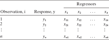
Throughout this chapter we assume that the regressor variables x₁, x₂,…, x_k are fixed (i.e., mathematical or nonrandom) variables, measured without error. However, just as was discussed in Section 2.12 for the simple linear regression model, all of our results are still valid for the case where the regressors are random variables. This is certainly important, because when regression data arise from an observational study, some or most of the regressors will be random variables. When the data result from a designed experiment, it is more likely that the x's will be fixed variables. When the x's are random variables, it is only necessary that the observations on each regressor be independent and that the distribution not depend on the regression coefficients (the β's) or on σ². When testing hypotheses or constructing CIs, we will have to assume that the conditional distribution of y given x₁, x₂,…, x_k be normal with mean β₀ + β₁x₁ + β₂x₂ + … + β_kx_k and variance σ².

We may write the sample regression model corresponding to Eq. (3.2) as

The least-squares function is

The function S must be minimized with respect to β₀, β₁,…, β_k. The least-squares estimators of β₀, β₁,…, β_k must satisfy

and

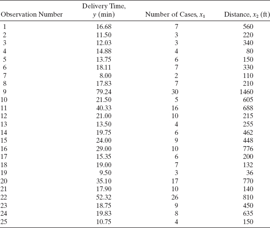
Simplifying Eq. (3.10), we obtain the least-squares normal equations

Note that there are p = k + 1 normal equations, one for each of the unknown regression coefficients. The solution to the normal equations will be the least-squares estimators .

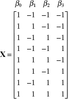
It is more convenient to deal with multiple regression models if they are expressed in matrix notation. This allows a very compact display of the model, data, and results. In matrix notation, the model given by Eq. (3.8) is

where

In general, y is an n × 1 vector of the observations, X is an n × p matrix of the levels of the regressor variables, β is a p × 1 vector of the regression coefficients, and ε is an n × 1 vector of random errors.

We wish to find the vector of least-squares estimators, , that minimizes

Note that S(β) may be expressed as

since β′X′y is a 1 × 1 matrix, or a scalar, and its transpose (β′X′y)′ = y′Xβ is the same scalar. The least-squares estimators must satisfy

which simplifies to

Equations (3.12) are the least-squares normal equations. They are the matrix analogue of the scalar presentation in (3.11).

To solve the normal equations, multiply both sides of (3.12) by the inverse of X′X. Thus, the least-squares estimator of β is

provided that the inverse matrix (X′X)⁻¹ exists. The (X′X)⁻¹ matrix will always exist if the regressors are linearly independent, that is, if no column of the X matrix is a linear combination of the other columns.

It is easy to see that the matrix form of the normal equations (3.12) is identical to the scalar form (3.11). Writing out (3.12) in detail, we obtain

If the indicated matrix multiplication is performed, the scalar form of the normal equations (3.11) is obtained. In this display we see that X′X is a p × p symmetric matrix and X′y is a p × 1 column vector. Note the special structure of the X′X matrix. The diagonal elements of X′X are the sums of squares of the elements in the columns of X, and the off-diagonal elements are the sums of cross products of the elements in the columns of X. Furthermore, note that the elements of X′y are the sums of cross products of the columns of X and the observations y_i.

The fitted regression model corresponding to the levels of the regressor variables x′ = [1,x₁, x₂,…,x_k] is

The vector of fitted values ŷ_i corresponding to the observed values y_i is

The n × n matrix H = X(X′X)⁻¹X′ is usually called the hat matrix. It maps the vector of observed values into a vector of fitted values. The hat matrix and its properties play a central role in regression analysis.

The difference between the observed value y_i and the corresponding fitted value ŷ_i is the residual e_i = y_i − ŷ_i. The n residuals may be conveniently written in matrix notation as

There are several other ways to express the vector of residuals e that will prove useful, including

Example 3.1 The Delivery Time Data

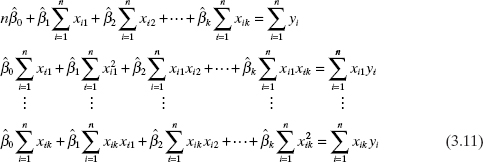
A soft drink bottler is analyzing the vending machine service routes in his distribution system. He is interested in predicting the amount of time required by the route driver to service the vending machines in an outlet. This service activity includes stocking the machine with beverage products and minor maintenance or house-keeping. The industrial engineer responsible for the study has suggested that the two most important variables affecting the delivery time (y) are the number of cases of product stocked (x₁) and the distance walked by the route driver (x₂). The engineer has collected 25 observations on delivery time, which are shown in Table 3.2. (Note that this is an expansion of the data set used in Example 2.9.) We will fit the multiple linear regression model

to the delivery time data in Table 3.2.

TABLE 3.2 Delivery Time Data for Example 3.1

Graphics can be very useful in fitting multiple regression models. Figure 3.4 is a scatterplot matrix of the delivery time data. This is just a two-dimensional array of two-dimensional plots, where (except for the diagonal) each frame contains a scatter diagram. Thus, each plot is an attempt to shed light on the relationship between a pair of variables. This is often a better summary of the relationships than a numerical summary (such as displaying the correlation coefficients between each pair of variables) because it gives a sense of linearity or nonlinearity of the relationship and some awareness of how the individual data points are arranged over the region.

When there are only two regressors, sometimes a three-dimensional scatter diagram is useful in visualizing the relationship between the response and the regressors. Figure 3.5 presents this plot for the delivery time data. By spinning these plots, some software packages permit different views of the point cloud. This view provides an indication that a multiple linear regression model may provide a reasonable fit to the data.

To fit the multiple regression model we first form the X matrix and y vector:

Figure 3.4 Scatterplot matrix for the delivery time data from Example 3.1.

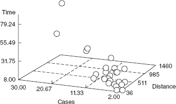
Figure 3.5 Three-dimensional scatterplot of the delivery time data from Example 3.1.

The X′X matrix is

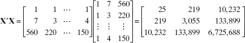
and the X′y vector is

The least-squares estimator of β is

or

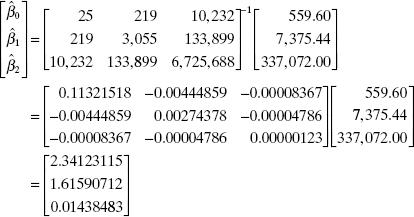
The least-squares fit (with the regression coefficients reported to five decimals) is

Table 3.3 shows the observations y_i along with the corresponding fitted values ŷ_i and the residuals e_i from this model.

Computer Output Table 3.4 presents a portion of the Minitab output for the soft drink delivery time data in Example 3.1. While the output format differs from one computer program to another, this display contains the information typically generated. Most of the output in Table 3.4 is a straightforward extension to the multiple regression case of the computer output for simple linear regression. In the next few sections we will provide explanations of this output information.

3.2.2 A Geometrical Interpretation of Least Squares

An intuitive geometrical interpretation of least squares is sometimes helpful. We may think of the vector of observations y′ = [y₁, y₁,…,y_n] as defining a vector from the origin to the point A in Figure 3.6. Note that y₁, y₂,…,y_n form the coordinates of an n-dimensional sample space. The sample space in Figure 3.6 is three-dimensional.

The X matrix consists of p(n × 1) column vectors, for example, 1 (a column vector of 1's), x₁, x₂,…, x_k. Each of these columns defines a vector from the origin in the sample space. These p vectors form a p-dimensional subspace called the estimation space. The estimation space for p = 2 is shown in Figure 3.6. We may represent any point in this subspace by a linear combination of the vectors 1, x₁,…, x_k. Thus, any point in the estimation space is of the form Xβ. Let the vector Xβ determine the point B in Figure 3.6. The squared distance from B to A is just

TABLE 3.3 Observations, Fitted Values, and Residuals for Example 3.1

TABLE 3.4 Minitab Output for Soft Drink Time Data

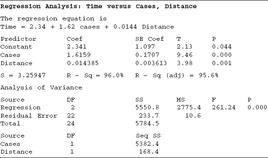
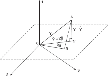
Figure 3.6 A geometrical interpretation of least squares.

Therefore, minimizing the squared distance of point A defined by the observation vector y to the estimation space requires finding the point in the estimation space that is closest to A. The squared distance is a minimum when the point in the estimation space is the foot of the line from A normal (or perpendicular) to the estimation space. This is point C in Figure 3.6. This point is defined by the vector Therefore, since is perpendicular to the estimation space, we may write

which we recognize as the least-squares normal equations.

3.2.3 Properties of the Least-Squares Estimators

The statistical properties of the least-squares estimator may be easily demonstrated. Consider first bias, assuming that the model is correct:

since E(ε) = 0 and (X′X)⁻¹X′X = I. Thus, is an unbiased estimator of β if the model is correct.

The variance property of is expressed by the covariance matrix

which is a p × p symmetric matrix whose jth diagonal element is the variance of and whose (ij)th off-diagonal element is the covariance between and . The covariance matrix of is found by applying a variance operator to :

Now (X′X)⁻¹X′ is a matrix of constants, and the variance of y is σ²I, so

Therefore, if we let C = (X′X)⁻¹, the variance of is σ²C_jj and the covariance between and is σ²C_ij.

Appendix C.4 establishes that the least-squares estimator is the best linear unbiased estimator of β (the Gauss-Markov theorem). If we further assume that the errors ε_i are normally distributed, then as we see in Section 3.2.6, is also the maximum-likelihood estimator of β. The maximum-likelihood estimator is the minimum variance unbiased estimator of β.

3.2.4 Estimation of σ²

As in simple linear regression, we may develop an estimator of σ² from the residual sum of squares

Substituting , we have

Since , this last equation becomes

Appendix C.3 shows that the residual sum of squares has n − p degrees of freedom associated with it since p parameters are estimated in the regression model. The residual mean square is

Appendix C.3 also shows that the expected value of MS_Res is σ², so an unbiased estimator of σ² is given by

As noted in the simple linear regression case, this estimator of σ² is model dependent.

Example 3.2 The Delivery Time Data

We now estimate the error variance σ² for the multiple regression model fit to the soft drink delivery time data in Example 3.1. Since

and

the residual sum of squares is

Therefore, the estimate of σ² is the residual mean square

The Minitab output in Table 3.4 reports the residual mean square as 10.6.

The model-dependent nature of this estimate σ² may be easily demonstrated. Table 2.12 displays the computer output from a least-squares fit to the delivery time data using only one regressor, cases(x_l). The residual mean square for this model is 17.5, which is considerably larger than the result obtained above for the two-regressor model. Which estimate is “correct”? Both estimates are in a sense correct, but they depend heavily on the choice of model. Perhaps a better question is which model is correct? Since σ² is the variance of the errors (the unexplained noise about the regression line), we would usually prefer a model with a small residual mean square to a model with a large one.

3.2.5 Inadequacy of Scatter Diagrams in Multiple Regression

We saw in Chapter 2 that the scatter diagram is an important tool in analyzing the relationship between y and x in simple linear regression. We also saw in Example 3.1 that a matrix of scatterplots was useful in visualizing the relationship between y and two regressors. It is tempting to conclude that this is a general concept; that is, examinjng scatter diagrams of y versus x_l, y versus x₂,…, y versus x_k is always useful in assessing the relationships between y and each of the regressors x_l, x₂,…, x_k. Unfortunately, this is not true in general.

Following Daniel and Wood [1980], we illustrate the inadequacy of scatter diagrams for a problem with two regressors. Consider the data shown in Figure 3.7. These data were generated from the equation

The matrix of scatterplots is shown in Figure 3.7. The y-versus-x₁, plot does not exhibit any apparent relationship between the two variables. The y-versus-x₁ plot indicates that a linear relationship exists, with a slope of approximately 8. Note that both scatter diagrams convey erroneous information. Since in this data set there are two pairs of points that have the same x₂ values (x₂ = 2 and x₂ = 4), we could measure the x₁ effect at fixed x₂ from both pairs. This gives, = (17−27)/(3−1) = −5 for x₂ = 2 and = (26−16)/(6−8) = −5 for x₂ = 4 the correct results. Knowing , we could now estimate the x₂ effect. This procedure is not generally useful, however, because many data sets do not have duplicate points.

Figure 3.7 A matrix of scatterplots.

This example illustrates that constructing scatter diagrams of y versus x_j, (j = 1, 2,…, k) can be misleading, even in the case of only two regressors operating in a perfectly additive fashion with no noise. A more realistic regression situation with several regressors and error in the y's would confuse the situation even further. If there is only one (or a few) dominant regressor, or if the regressors operate nearly independently, the matrix of scatterplots is most useful. However, when several important regressors are themselves interrelated, then these scatter diagrams can be very misleading. Analytical methods for sorting out the relationships between several regressors and a response are discussed in Chapter 10.

3.2.6 Maximum-Likelihood Estimation

Just as in the simple linear regression case, we can show that the maximum-likelihood estimators for the model parameters in multiple linear regression when the model errors are normally and independently distributed are also least-squares estimators. The model is

and the errors are normally and independently distributed with constant variance σ², or ε is distributed as N(0, σ²I). The normal density function for the errors is

The likelihood function is the joint density of . Therefore, the likelihood function is

Now since we can write ε = y − Xβ, the likelihood function becomes

As in the simple linear regression case, it is convenient to work with the log of the likelihood,

It is clear that for a fixed value of 0 the log-likelihood is maximized when the term

is minimized. Therefore, the maximum-likelihood estimator of β under normal errors is equivalent to the least-squares estimator . The maximum-likelihood estimator of σ² is

These are multiple linear regression generalizations of the results given for simple linear regression in Section 2.11. The statistical properties of the maximum-likelihood estimators are summarized in Section 2.11.

3.3 HYPOTHESIS TESTING IN MULTIPLE LINEAR REGRESSION

Once we have estimated the parameters in the model, we face two immediate questions:

1. What is the overall adequacy of the model?
2. Which specific regressors seem important?

Several hypothesis testing procedures prove useful for addressing these questions. The formal tests require that our random errors be independent and follow a normal distribution with mean E(ε_i) = 0 and variance Var(ε_i) = σ².

3.3.1 Test for Significance of Regression

he test for significance of regression is a test to determine if there is a linear relationship between the response y and any of the regressor variables x₁, x₂,…, x_k. This procedure is often thought of as an overall or global test of model adequacy. The appropriate hypotheses are

Rejection of this null hypothesis implies that at least one of the regressors x₁, x₂,…, x_k contributes significantly to the model.

The test procedure is a generalization of the analysis of variance used in simple linear regression. The total sum of squares SS_T is partitioned into a sum of squares due to regression, SS_R, and a residual sum of squares, SS_Res. Thus,

Appendix C.3 shows that if the null hypothesis is true, then SS_R/σ² follows a χ²_k distribution, which has the same number of degrees of freedom as number of regressor variables in the model. Appendix C.3 also shows that and that SS_Res and SS_R are independent. By the definition of an F statistic given in Appendix C.1,

follows the F_k,n−k−1 distribution. Appendix C.3 shows that

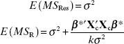
where β* = (β₁, β₂,…, β_k)′ and X_c is the “centered” model matrix given by

These expected mean squares indicate that if the observed value of F₀ is large, then it is likely that at least one β_j ≠ 0. Appendix C.3 also shows that if at least one β_j ≠ 0 then F₀ follows a noncentral F distribution with k and n − k − 1 degrees of freedom and a noncentrality parameter of

This noncentrality parameter also indicates that the observed value of F₀ should be large if at least one β_j ≠ 0. Therefore, to test the hypothesis H₀: β₁ = β₂ = … = β_k = 0 compute the test statistic F₀ and reject H₀ if

The test procedure is usually summarized in an analysis-or-variance table such as Table 3.5.

A computational formula for SS_R is found by starting with

TABLE 3.5 Analysis of Variance for Significance of Regression in Multiple Regression

and since

we may rewrite the above equation as

or

Therefore, the regression sum of squares is

the residual sum of squares is

and the total sum of squares is

Example 3.3 The Delivery Time Data

We now test for significance of regression using the delivery time data from Example 3.1. Some of the numerical quantities required are calculated in Example 3.2. Note that

and

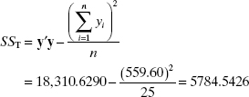
The analysis of variance is shown in Table 3.6. To test H₀: β₁ = β₂ = 0, we calculate the statistic

Since the P value is very small, we conclude that delivery time is related to delivery volume and/or distance. However, this does not necessarily imply that the relationship found is an appropriate one for predicting delivery time as a function of volume and distance. Further tests of model adequacy are required.

Minitab Output The MlNITAB output in Table 3.4 also presents the analysis of variance for testing significance of regression. Apart from rounding, the results are in agreement with those reported in Table 3.6.

R² and Adjusted R² Two other ways to assess the overall adequacy of the model are R² and the adjusted R², denoted R²_Adj. The MlNITAB output in Table 3.4 reports the R² for the multiple regression model for the delivery time data as R² = 0.96, or 96.0%. In Example 2.9, where only the single regressor x₁ (cases) was used, the value of R² was smaller, namely R² = 0.93, or 93.0% (see Table 2.12). In general, R² never decreases when a regressor is added to the model, regardless of the value of the contribution of that variable. Therefore, it is difficult to judge whether an increase in R² is really telling us anything important.

Some regression model builders prefer to use an adjusted R² statistic, defined as

TABLE 3.6 Test for Significance of Regression for Example 3.3

Since SS_Res/(n − p) is the residual mean square and SS_T/(n − 1) is constant regardless of how many variables are in the model, R²_Adj will only increase on adding a variable to the model if the addition of the variable reduces the residual mean square. Minitab (Table 3.4) reports R²_Adj = 0.956 (95.6%) for the two-variable model, while for the simple linear regression model with only x₁ (cases), R²_Adj = 0.927, or 92.7% (see Table 2.12). Therefore, we would conclude that adding x₂ (distance) to the model did result in a meaningful reduction of total variability.

In subsequent chapters, when we discuss model building and variable selection, it is frequently helpful to have a procedure that can guard against overfitting the model, that is, adding terms that are unnecessary. The adjusted R² penalizes us for adding terms that are not helpful, so it is very useful in evaluating and comparing candidate regression models.

3.3.2 Tests on Individual Regression Coefficients and Subsets of Coefficients

Once we have determined that at least one of the regressors is important, a logical question becomes which one(s). Adding a variable to a regression model always causes the sum of squares for regression to increase and the residual sum of squares to decrease. We must decide whether the increase in the regression sum of squares is sufficient to warrant using the additional regressor in the model. The addition of a regressor also increases the variance of the fitted value ŷ, so we must be careful to include only regressors that are of real value in explaining the response. Furthermore, adding an unimportant regressor may increase the residual mean square, which may decrease the usefulness of the model.

The hypotheses for testing the significance of any individual regression coefficient, such as β_j are

If H₀: β_j = 0, is not rejected, then this indicates that the regressor x_j, can be deleted from the model. The test statistic for this hypothesis is

where C_jj is the diagonal element of (X′X)⁻¹ corresponding to . The null hypothesis H₀: β_j = 0 is rejected if |t₀|>t_{α/2,n−1k−1}. Note that this is really a partial or marginal test because the regression coefficient depends on all of the other regressor variables x_i(i ≠ j) that are in the model. Thus, this is a test of the contribution of x_j, given the other regressors in the model.

Example 3.4 The Delivery Time Data

To illustrate the procedure, consider the delivery time data in Example 3.1. Suppose we wish to assess the value of the regressor variable x₂ (distance) given that the regressor x₁ (cases) is in the model. The hypotheses are

The main diagonal element of (X′X)⁻¹ corresponding to β₂ is C₂₂ = 0.00000123, so the t statistic (3.29) becomes

Since t_0.025,22 = 2.074, we reject H₀: β₂ = 0 and conclude that the regressor x₂ (distance) contributes significantly to the model given that x₁ (cases) is also in the model. This t test is also provided in the Minitab output (Table 3.4), and the P value reported is 0.001.

We may also directly determine the contribution to the regression sum of squares of a regressor, for example, x_j, given that other regressors x₁(i ≠ j) are included in the model by using the extra-sum-of-squares method. This procedure can also be used to investigate the contribution of a subset of the regressor variables to the model.

Consider the regression model with k regressors

where y is n × 1 X is n × p, β is p × 1 ε is n × 1, and p = k + 1. We would like to determine if some subset of r < k regressors contributes significantly to the regression model. Let the vector of regression coefficients be partitioned as follows:

where β₁ is (p − r) × 1 and β₂ is r × 1. We wish to test the hypotheses

The model may be written as

where the n × (p − r) matrix X_l represents the columns of X associated with β₁ and the n × r matrix X₂ represents the columns of X associated with β₂. This is called the full model.

For the full model, we know that . The regression sum of squares for this model is

and

To find the contribution of the terms in β₂ to the regression, fit the model assuming that the null hypothesis H₀: β₂ = 0 is true. This reduced model is

The least-squares estimator of β₁ in the reduced model is . The regression sum of squares is

The regression sum of squares due to β₁ given that β₂ is already in the model is

with p − (p − r) = r degrees of freedom. This sum of squares is called the extra sum of squares due to β₂ because it measures the increase in the regression sum of squares that results from adding the regressors X_{k − r+1}, X_{k − r+2},…, X_k to a model that already contains x₁, x₂,…, x_k−r. Now SS_R(β₂|β₁) is independent of MS_Res, and the null hypothesis β₂ = 0 may be tested by the statistic

If β₂ ≠ 0, then F₀ follows a noncentral F distribution with a noncentrality parameter of

This result is quite important. If there is multicollinearity in the data, there are situations where β₂ is markedly nonzero, but this test actually has almost no power (ability to indicate this difference) because of a near-collinear relationship between X₁ and X₂. In this situation, λ is nearly zero even though β₂ is truly important. This relationship also points out that the maximal power for this test occurs when X₁ and X₂, are orthogonal to one another. By orthogonal we mean that X′₂X₁ = 0.

If F₀ > F_α,r,n−p, we reject H₀, concluding that at least one of the parameters in β₂ is not zero, and consequently at least one of the regressors x_k−r+1, x_k−r+2,…, x_k in X₂ contribute significantly to the regression model. Some authors call the test in (3.35) a partial F test because it measures the contribution of the regressors in X₂ given that the other regressors in X₁ are in the model. To illustrate the usefulness of this procedure, consider the model

The sums of squares

are single-degree-of-freedom sums of squares that measure the contribution of each regressor x_j, j = 1, 2, 3, to the model given that all of the other regressors were already in the model. That is, we are assessing the value of adding x_j to a model that did not include this regressor. In general, we could find

which is the increase in the regression sum of squares due to adding x_j to a model that already contains x₁,…, x_j−1x_j+1,… x_k. Some find it helpful to think of this as measuring the contribution of x_j as if it were the last variable added to the model.

Appendix C3.35 formally shows the equivalence of the partial F test on a single variable x_j and the t test in (3.29). However, the partial F test is a more general procedure in that we can measure the effect of sets of variables. In Chaper 10 we will show how the partial F test plays a major role in model building, that is, in searching for the best set of regressors to use in the model.

The extra-sum-of-squares method can be used to test hypotheses about any subset of regressor variables that seems reasonable for the particular problem under analysis. Sometimes we find that there is a natural hierarchy or ordering in the regressors, and this forms the basis of a test. For example, consider the quadratic polynomial

Here we might be interested in finding

which would measure the contribution of the first-order terms to the model, and

which would measure the contribution of adding second-order terms to a model that already contained first-order terms.

When we think of adding regressors one at a time to a model and examining the contribution of the regressor added at each step given all regressors added previously, we can partition the regression sum of squares into marginal single-degree-of-freedom components. For example, consider the model

with the corresponding analysis-of-variance identity

We may decompose the three-degree-of-freedom regression sum of squares as follows:

where each sum of squares on the right-hand side has one degree of freedom. Note that the order of the regressors in these marginal components is arbitrary. An alternate partitioning of SS_R(β₁, β₂, β₃|β₀) is

However, the extra-sum-of-squares method does not always produce a partitioning of the regression sum of squares, since, in general,

Minitab Output The Minitab output in Table 3.4 provides a sequential partitioning of the regression sum of squares for x₁ = cases and x₂ = distance. The reported quantities are

Example 3.5 The Delivery Time Data

Consider the soft drink delivery time data in Example 3.1. Suppose that we wish to investigate the contribution of the variable distance (x₂) to the model. The appropriate hypotheses are

To test these hypotheses, we need the extra sum of squares due to β₂, or

From Example 3.3 we know that

The reduced model y = β₀ + β₁x₁ + ε was fit in Example 2.9, resulting in ŷ = 3.3208 + 2.1762x₁. The regression sum of squares for this model is

Therefore, we have

This is the increase in the regression sum of squares that results from adding x₂ to a model already containing x₁. To test H₀: β₂ = 0, form the test statistic

Note that the MS_Res from the full model using both x₁ and x₂ is used in the denominator of the test statistic. Since F_0.05,1,22 = 4.30, we reject H₀: β₂ = 0 and conclude that distance (x₂) contributes significantly to the model.

Since this partial F test involves a single variable, it is equivalent to the t test. To see this, recall that the t test on H₀: β₂ = 0 resulted in the test statistic t₀ = 3.98. From Section C.1, the square of a t random variable with v degrees of freedom is an F random variable with one numerator and v denominator degrees of freedom, and we have t₀² = (3.98)² = 15.84 ≃ F₀

3.3.3 Special Case of Orthogonal Columns in X

Consider the model (3.31)

The extra-sum-of-squares method allows us to measure the effect of the regressors in X₂ conditional on those in X₁ by computing SS_R(β₂|β₁). In general, we cannot talk about finding the sum of squares due to β₂, SS_R(β₂), without accounting for the dependence of this quantity on the regressors in X₁. However, if the columns in X₁ are orthogonal to the columns in X₂, we can determine a sum of squares due to β₂ that is free of any dependence on the regressors in X₁.

To demonstrate this, form the normal equations for the model (3.31). The normal equations are

Now if the columns of X₁ are orthogonal to the columns in X₂, X′₁X₂ = 0 and X′₂X₁ = 0. Then the normal equations become

with solution

Note that the least-squares estimator of β₁ is regardless of whether or not X₂ is in the model, and the least-squares estimator of β₂ is regardless of whether or not X₁ is in the model.

The regression sum of squares for the full model is

However, the normal equations form two sets, and for each set we note that

Comparing Eq. (3.37) with Eq. (3.36), we see that

Therefore,

and

Consequently, SS_R(β₁) measures the contribution of the regressors in X₁ to the model unconditionally, and SS_R(β₂) measures the contribution of the regressors in X₂ to the model unconditionally. Because we can unambiguously determine the effect of each regressor when the regressors are orthogonal, data collection experiments are often designed to have orthogonal variables.

As an example of a regression model with orthogonal regressors, consider the model y = β₀ + β₁x₁ + β₂x₂ + β₃x₃ + ε where the X matrix is

The levels of the regressors correspond to the 2³ factorial design. It is easy to see that the columns of X are orthogonal. Thus, SS_R(β_j), j = 1, 2, 3, measures the contribution of the regressor x_j, to the model regardless of whether any of the other regressors are included in the fit.

3.3.4 Testing the General Linear Hypothesis

Many hypotheses about regression coefficients can be tested using a unified approach. The extra-sum-of-squares method is a special case of this procedure. In the more general procedure the sum of squares used to test the hypothesis is usually calculated as the difference between two residual sums of squares. We will now outline the procedure. For proofs and further discussion, refer to Graybill [1976], Searle [1971], or Seber [1977].

Suppose that the null hypothesis of interest can be expressed as H₀: Tβ = 0, where T is an m × p matrix of constants, such that only r of the m equations in Tβ = 0 are independent. The full model is y = Xβ + ε, with = (X′X)⁻¹X′y, and the residual sum of squares for the full model is

To obtain the reduced model, the r independent equations in Tβ = 0 are used to solve for r of the regression coefficients in the full model in terms of the remaining p − r regression coefficients. This leads to the reduced model y = Zγ + ε, for example, where Z is an n × (p − r) matrix and γ is a (p − r) × 1 vector of unknown regression coefficients. The estimate of γ is

and the residual sum of squares for the reduced model is

The reduced model contains fewer parameters than the full model, so consequently SS_Res(RM) ≥ SS_Res(FM). To test the hypothesis H₀: Tβ = 0, we use the difference in residual sums of squares

with n − p + r − (n − p) = r degrees of freedom. Here SS_H is called the sum of squares due to the hypothesis H₀: Tβ = 0. The test statistic for this hypothesis is

We reject H₀: Tβ = 0 if F₀ > F_α,r,n−p.

Example 3.6 Testing Equality of Regression Coefficients

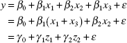
The general linear hypothesis approach can be used to test the equality of regression coefficients. Consider the model

For the full model, SS_Res(RM) has n − p = n − 4 degrees of freedom. We wish to test H₀: β₁ = β₃. This hypothesis may be stated as H₀: Tβ = 0, where

is a 1 × 4 row vector. There is only one equation in Tβ = 0, namely, β₁ − β₃ = 0. Substituting this equation into the full model gives the reduced model

where γ₀ = β₀, γ₁ = β₁(=β₃), z₁ = x₁ + x₃, γ₂ = β₂, and z₂ = x₂. We would find SS_Res(RM) with n − 4 + 1 = n − 3 degrees of freedom by fitting the reduced model. The sum of squares due to hypothesis SS_H = SS_Res(RM) − SS_Res(FM) has n − 3 − (n − 4) = 1 degree of freedom. The F ratio (3.40) is F₀ = (SS_H/1)[SS_Res(RM)/(n − 4)]. Note that this hypothesis could also be tested by using the t statistic

with n − 4 degrees of freedom. This is equivalent to the F test.

Example 3.7

Suppose that the model is

and we wish to test H₀: β₁ = β₃, β₂ = 0. To state this in the form of the general linear hypothesis, let

There are now two equations in Tβ = 0, β₁ − β₃ = 0 and β₂ = 0. These equations give the reduced model

In this example,SS_Res(RM) has n − 2 degrees of freedom, so SS_R has n − 2 − (n − 4) = 2 degrees of freedom. The F ratio (3.40) is F₀ = (SS_H/2)/[SS_Res(FM)/(n − 4)].

The test statistic (3.40) for the general linear hypothesis may be written in another form, namely,

This form of the statistic could have been used to develop the test procedures illustrated in Examples 3.6 and 3.7.

There is a slight extension of the general linear hypothesis that is occasionally useful. This is

for which the test statistic is

Since under the null hypothesis Tβ = c, the distribution of F₀ in Eq. (3.43) is F_r,n−p, we would reject H₀: Tβ = c if F₀ > F_α,r,n−p. That is, the test procedure is an upper one-tailed F test. Notice that the numerator of Eq. (3.43) expresses a measure of squared distance between Tβ and c standardized by the covariance matrix of .

To illustrate how this extended procedure can be used, consider the situation described in Example 3.6, and suppose that we wish to test

Clearly T = [0,1,0, −1] and c = [2]. For other uses of this procedure, refer to Problems 3.21 and 3.22.

Finally, if the hypothesis H₀: Tβ = 0 (or H₀: Tβ = c) cannot be rejected, then it may be reasonable to estimate β subject to the constraint imposed by the null hypothesis. It is unlikely that the usual least-squares estimator will automatically satisfy the constraint. In such cases a constrained least-squares estimator may be useful. Refer to Problem 3.34.

3.4 CONFIDENCE INTERVALS IN MULTIPLE REGRESSION

Confidence intervals on individual regression coefficients and confidence intervals on the mean response given specific levels of the regressors play the same important role in multiple regression that they do in simple linear regression. This section develops the one-at-a-time confidence intervals for these cases. We also briefly introduce simultaneous confidence intervals on the regression coefficients.

3.4.1 Confidence Intervals on the Regression Coefficients

To construct confidence interval estimates for the regression coefficients β_j we will continue to assume that the errors ε_i are normally and independently distributed with mean zero and variance σ². Therefore, the observations y_i are normally and independently distributed with mean and variance σ². Since the least-squares estimator is a linear combination of the observations, it follows that is normally distributed with mean vector β and covariance matrix σ²(X′X)⁻¹. This implies that the marginal distribution of any regression coefficient is normal with mean β_j and variance σ²C_jj, where C_jj is the jth diagonal element of the (X′X)⁻¹ matrix. Consequently, each of the statistics

is distributed as t with n − p degrees of freedom, where is the estimate of the error variance obtained from Eq. (3.18).

Based on the result given in Eq. (3.44), we may defme a 100(1 − α) percent confidence interval for the regression coefficient β_j, j = 0, 1,…,k, as

Remember that we call the quantity

the standard error of the regression coefficient .

Example 3.8 The Delivery Time Data

We now find a 95% CI for the parameter β₁ in Example 3.1. The point estimate of β₁ is = 1.61591, the diagonal element of (X′X)⁻¹ corresponding to β₁ is C₁₁ = 0.00274378, and = 10.6239 (from Example 3.2). Using Eq. (3.45), we find that

and the 95% CI on β₁ is

Notice that the Minitab output in Table 3.4 gives the standard error of each regression coefficient. This makes the construction of these intervals very easy in practice.

3.4.2 CI Estimation of the Mean Response

We may construct a CI on the mean response at a particular point, such as x₀₁, x₀₂,…,x_0k. Define the vector x₀ as

The fitted value at this point is

This is an unbiased estimator of E(y|x₀), since E(ŷ₀) = x′₀β = E(y|x₀), and the variance of ŷ₀ is

Therefore, a 100(1 − α) percent confidence interval on the mean response at the point x₀₁, x₀₂,…,x_0k is

This is the multiple regression generalization of Eq. (2.43).

Example 3.9 The Delivery Time Data

The soft drink bottler in Example 3.1 would like to construct a 95% CI on the mean delivery time for an outlet requiring x₁ = 8 cases and where the distance x₂ = 275 feet. Therefore,

The fitted value at this point is found from Eq. (3.47) as

The variance of ŷ₀ is estimated by

Therefore, a 95% CI on the mean delivery time at this point is found from Eq. (3.49) as

which reduces to

Ninety-five percent of such intervals will contain the true delivery time.

The length of the CI or the mean response is a useful measure of the quality of the regression model. It can also be used to compare competing models. To illustrate, consider the 95% CI on the the mean delivery time when x₁ = 8 cases and x₂ = 275 feet. In Example 3.9 this CI is found to be (17.66, 20.78), and the length of this interval is 20.78 − 17.16 = 3.12 minutes. If we consider the simple linear regression model with = cases as the only regressor, the 95% CI on the mean delivery time with x₁ = 8 cases is (18.99, 22.97). The length of this interval is 22.47 − 18.99 = 3.45 minutes. Clearly, adding cases to the model has improved the precision of estimation. However, the change in the length of the interval depends on the location of the point in the x space. Consider the point x₁ = 16 cases and x₂ = 688 feet. The 95% CI for the multiple regression model is (36.11, 40.08) with length 3.97 minutes, and for the simple linear regression model the 95% CI at x₁ = 16 cases is (35.60, 40.68) with length 5.08 minutes. The improvement from the multiple regression model is even better at this point. Generally, the further the point is from the centroid of the x space, the greater the difference will be in the lengths of the two CIs.

3.4.3 Simultaneous Confidence Intervals on Regression Coefficients

We have discussed procedures for constructing several types of confidence and prediction intervals for the linear regression model. We have noted that these are one-at-a-time intervals, that is, they are the usual type of confidence or prediction interval where the confidence coefficient 1 − α indicates the proportion of correct statements that results when repeated random samples are selected and the appropriate interval estimate is constructed for each sample. Some problems require that several confidence or prediction intervals be constructed using the same sample data. In these cases, the analyst is usually interested in specifying a confidence coefficient that applies simultaneously to the entire set of interval estimates. A set of confidence or prediction intervals that are all true simultaneously with probability 1 − α are called simultaneous or joint confidence or joint prediction intervals.

As an example, consider a simple linear regression model. Suppose that the analyst wants to draw inferences about the intercept β₀ and the slope β₁. One possibility would be to construct 95% (say) CIs about both parameters. However, if these interval estimates are independent, the probability that both statements are correct is (0.95)² = 0.9025. Thus, we do not have a confidence level of 95% associated with both statements. Furthermore, since the intervals are constructed using the same set of sample data, they are not independent. This introduces a further complication into determining the confidence level for the set of statements.

It is relatively easy to define a joint confidence region for the multiple regression model parameters β. We may show that

and this implies that

Consequently, a 100(1 − α) percent joint confidence region for all of the parameters in β

This inequality describes an elliptically shaped region. Construction of this joint confidence region is relatively straightforward for simple linear regression (p = 2). It is more difficult for p = 3 and would require special three-dimensional graphics software.

Example 3.10 The Rocket Propellant Data

For the case of simple linear regression, we can show that Eq. (3.50) reduces to

To illustrate the construction of this confidence region, consider the rocket propellant data in Example 2.1. We will find a 95% confidence region for β₀ and β₁. , and F_0.05,2,18 = 3.55, we may substitute into the above equation, yielding

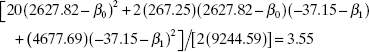
as the boundary of the ellipse.

Figure 3.8 Joint 95% confidence region for β₀ and β₁ for the rocket propellant data.

The joint confidence region is shown in Figure 3.8. Note that this ellipse is not parallel to the β₁ axis. The tilt of the ellipse is a function of the covariance between β₁ and β₂, which is −σ²/S_xx. A positive covariance implies that errors in the point estimates of β₀ and β₁ are likely to be in the same direction, while a negative covariance indicates that these errors are likely to be in opposite directions. In our example is positive so Cov(, ) is negative. Thus, if the estimate of the slope is too steep (β₁ is overestimated), the estimate of the intercept is likely to be too small (β₀ is underestimated). The elongation of the region depends on the relative sizes of the variances of β₀ and β₁. Generally, if the ellipse is elongated in the β₀ direction (for example), this implies that β₀ is not estimated as precisely as β₁. This is the case in our example.

There is another general approach for obtaining simultaneous interval estimates of the parameters in a linear regression model. These CIs may be constructed by using

where the constant Δ is chosen so that a specified probability that all intervals are correct is obtained.

Several methods may be used to choose Δ in (3.51). One procedure is the Bonferroni method. In this approach, we set Δ = t_α/2p,n−p, so that (3.51) becomes

The probability is at least 1 − α that all intervals are correct. Notice that the Bonferroni confidence intervals look somewhat like the ordinary one-at-a-time CIs based on the t distribution, except that each Bonferroni interval has a confidence coefficient 1 − α/p instead of 1 − α.

Example 3.11 The Rocket Propellant Data

We may find 90% joint CIs for β₀ and β₁ for the rocket propellant data in Example 2.1 by constructing a 95% CI for each parameter. Since

and t_0.05/2,18 = t_0.025,18 = 2.101, the joint CIs are

and

We conclude with 90% confidence that this procedure leads to correct interval estimates for both parameters.

The confidence ellipse is always a more efficient procedure than the Bonferroni method because the volume of the ellipse is always less than the volume of the space covered by the Bonferroni intervals. However, the Bonferroni intervals are easier to construct.

Constructing Bonferroni CIs often requires significance levels not listed in the usual t tables. Many modern calculators and software packages have values of t_a,v on call as a library function.

The Bonferroni method is not the only approach to choosing Δ in (3.51). Other approaches include the Scheffé S-method (see Scheffé [1953, 1959]), for which

and the maximum modulus t procedure (see Hahn [1972] and Hahn and Hendrickson [1971]), for which

where u_a,p,n−p is the upper α-tail point of the distnbution of the maximum absolute value of two independent student t random variables each based on n − 2 degrees of freedom. An obvious way to compare these three techniques is in terms of the lengths of the CIs they generate. Generally the Bonferroni intervals are shorter than the Scheffé intervals and the maximum modulus t intervals are shorter than the Bonferroni intervals.

3.5 PREDICTION OF NEW OBSERVATIONS

The regression model can be used to predict future observations on y corresponding to particular values of the regressor variables, for example, x₀₁, x₀₂,…, x₀, x_0k. If X′₀ = [1,x₀₁, x₀₂,…, x₀, x_0k], then a point estimate of the future observation y₀ at the point x₀₁, x₀₂,…, x₀, x_0k is

A 100(1 − α) percent prediction interval for this future observation is

This is a generalization of the prediction interval for a future observation in simple linear regression, (2.45).

Example 3.12 The Delivery Time Data

Suppose that the soft drink bottler in Example 3.1 wishes to construct a 95% prediction interval on the delivery time at an outlet where x₁ = 8 cases are delivered and the distance walked by the deliveryman is x₂ = 275 feet. Note that x′₀ = [1, 8, 275], and the point estimate of the delivery time is ŷ₀ = x′₀ = 19.22 minutes. Also, in Example 3.9 we calculated x′₀(X′X)⁻¹x₀ = 0.05346. Therefore, from (3.54) we have

and the 95% prediction interval is

3.6 A MULTIPLE REGRESSION MODEL FOR THE PATIENT SATISFACTION DATA

In Section 2.7 we introduced the hospital patient satisfaction data and built a simple linear regression model relating patient satisfaction to a severity measure of the patient's illness. The data used in this example is in Table B17. In the simple linear regression model the regressor severity was significant, but the model fit to the data wasn't entirely satisfactory. Specifically, the value of R² was relatively low, approximately 0.43, We noted that there could be several reasons for a low value of R², including missing regressors. Figure 3.9 is the JMP output that results when we fit a multiple linear regression model to the satisfaction response using severity and patient age as the predictor variables.

In the multiple linear regression model we notice that the plot of actual versus predicted response is much improved when compared to the plot for the simple linear regression model (compare Figure 3.9 to Figure 2.7). Furthermore, the model is significant and both variables, age and severity, contribute significantly to the model. The R² has increased from 0.43 to 0.81. The mean square error in the multiple linear regression model is 90.74, considerably smaller than the mean square error in the simple linear regression model, which was 270.02. The large reduction in mean square error indicates that the two-variable model is much more effective in explaining the variability in the data than the original simple linear regression model. This reduction in the mean square error is a quantitative measure of the improvement we qualitatively observed in the plot of actual response versus the predicted response when the predictor age was added to the model. Finally, the response is predicted with better precision in the multiple linear model. For example, the standard deviation of the predicted response for a patient that is 42 year old with a severity index of 30 is 3.10 for the multiple linear regression model while it is 5.25 for the simple linear regression model that includes only severity as the predictor. Consequently the prediction interval would be considerably wider for the simple linear regression model. Adding an important predictor to a regression model (age in this example) can often result in a much better fitting model with a smaller standard error and as a consequence narrow confidence intervals on the mean response and narrower prediction intervals.

Figure 3.9 JMP output for the multiple linear regression model for the patient satisfaction data.

3.7 USING SAS AND R FOR BASIC MULTIPLE LINEAR REGRESSION

SAS is an important statistical software package. Table 3.7 gives the source code to analyze the delivery time data that we have been analyzing throughout this chapter. The statement PROC REG tells the software that we wish to perform an ordinary least-squares linear regression analysis. The “model” statement gives the specific model and tells the software which analyses to perform. The commands for the optional analyses appear after the solidus. PROC REG always produces the analysis-of-variance table and the information on the parameter estimates. The “p clm cli” options on the model statement produced the information on the predicted values. Specifically, “p” asks SAS to print the predicted values, “clm” (which stands for confidence limit, mean) asks SAS to print the confidence band, and “cli” (which stands for confidence limit, individual observations) asks to print the prediction band. Table 3.8 gives the resulting output, which is consistent with the Minitab analysis.

TABLE 3.7 SAS Code for Delivery Time Data

We next illustrate the R code required to do the same analysis. The first step is to create the data set. The easiest way is to input the data into a text file using spaces for delimiters. Each row of the data file is a record. The top row should give the names for each variable. All other rows are the actual data records. Let delivery.txt be the name of the data file. The first row of the text file gives the variable names:

time cases distance

The next row is the first data record, with spaces delimiting each data item:

16.68 7 560

The R code to read the data into the package is:

deliver <-read.table(“delivery.txt”, header = TRUE, sep = “”)

The object deliver is the R data set, and “delivery.txt” is the original data file. The phrase, hearder = TRUE tells R that the first row is the variable names. The phrase sep = “” tells R that the data are space delimited.

The commands

deliver.model <- lm(time~cases + distance, data = deliver)
summary(deliver.model)

tell R

• to estimate the model, and
• to print the analysis of variance, the estimated coefficients, and their tests.

3.8 HIDDEN EXTRAPOLATION IN MULTIPLE REGRESSION

In predicting new responses and in estimating the mean response at a given point x₀₁, x₀₂,…,x_0k one must be careful about extrapolating beyond the region containing the original observations. It is very possible that a model that fits well in the region of the original data will perform poorly outside that region. In multiple regression it is easy to inadvertently extrapolate, since the levels of the regressors (x_i1, x_i2,…,x_ik), i = 1, 2,…n, jointly define the region containing the data. As an example, consider Figure 3.10, which illustrates the region containing the original data for a two-regressor model. Note that the point (x₀₁, x₀₂) lies within the ranges of both regressors x₁ and x₂ but outside the region of the original data. Thus, either predicting the value of a new observation or estimating the mean response at this point is an extrapolation of the original regression model.

TABLE 3.8 SAS Output for the Analysis of Delivery Time Data

Figure 3.10 An example of extrapolation in multiple regression.

Since simply comparing the levels of the x's for a new data point with the ranges of the original x's will not always detect a hidden extrapolation, it would be helpful to have a formal procedure to do so. We will define the smallest convex set containing all of the original n data points (x_i1, x_i2,…, x_ik), i = 1, 2, …, n, as the regressor variable hull (RVH). If a point x₀₁, x₀₂,…,x_0k lies inside or on the boundary of the RVH, then prediction or estimation involves interpolation, while if this point lies outside the RVH, extrapolation is required.

The diagonal elements h_ii of the hat matrix H = X(X′X)⁻¹X′ are useful in detecting hidden extrapolation. The values of h_ii depend both on the Euclidean distance of the point x_i from the centroid and on the density of the points in the RVH. In general, the point that has the largest value of h_ii, say h_max, will lie on the boundary of the RVH in a region of the x space where the density of the observations is relatively low. The set of points x (not necessarily data points used to fit the model) that satisfy

is an ellipsoid enclosing all points inside the RVH (see Cook [1979] and Weisberg [1985]). Thus, if we are interested in prediction or estimation at the point x′₀ = [1, x₀₁, x₀₂,…, x_0k], the location of that point relative to the RVH is reflected by

Points for which h₀₀ > h_max are outside the ellipsoid enclosing the RVH and are extrapolation points. However, if h₀₀ < h_max, then the point is inside the ellipsoid and possibly inside the RVH and would be considered an interpolation point because it is close to the cloud of points used to fit the model. Generally the smaller the value of h₀₀, the closer the point x₀ lies to the centroid of the x space.^†

Weisberg [1985] notes that this procedure does not produce the smallest volume ellipsoid containing the RVH. This is called the minimum covering ellipsoid (MCE). He gives an iterative algorithm for generating the MCE. However, the test for extrapolation based on the MCE is still only an approximation, as there may still be regions inside the MCE where there are no sample points.

Example 3.13 Hidden Extrapolation—The Delivery Time Data

We illustrate detecting hidden extrapolation using the soft drink delivery time data in Example 3.1. The values of h_ii for the 25 data points are shown in Table 3.9. Note that observation 9, represented by ⋄ in Figure 3.11, has the largest value of h_ii. Figure 3.11 confirms that observation 9 is on the boundary of the RVH.

Now suppose that we wish to consider prediction or estimation at the following four points:

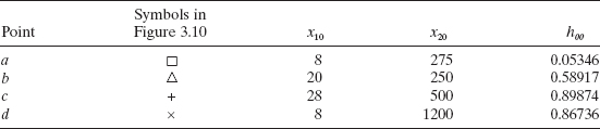
All of these points lie within the ranges of the regressors x₁ and x₂. In Figure 3.11 point a (used in Examples 3.9 and 3.12 for estimation and prediction), for which h₀₀ = 0.05346, is an interpolation point since h₀₀ = 0.05346 < h_max = 0.49829. The remaining points b, c, and d are all extrapolation points, since their values of h₀₀ exceed h_max. This is readily confirmed by inspection of Figure 3.11.

3.9 STANDARDIZED REGRESSION COEFFLCIENTS

It is usually difficult to directly compare regression coefficients because the maguitude of reflects the units of measurement of the regressor x_j. For example, suppose that the regression model is

TABLE 3.9 Values of h_ii for the Delivery Time Data

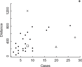
Figure 3.11 Scatterplot of cases and distance for the delivery time data.

and y is measured in liters, x₁ is measured in milliliters, and x₂ is measured in liters. Note that although is considerably larger than , the effect of both regressors on y is identical, since a 1-liter change in either x₁ or x₂ when the other variable is held constant produces the same change in y. Generally the units of the regression coefficient β_j are units of y/units of x_j,. For this reason, it is sometimes helpful to work with scaled regressor and response variables that produce dimensionless regression coefficients. These dimensionless coefficients are usually called standardized regression coefficients. We now show how they are computed, using two popular scaling techniques.

Unit Normal Scaling The first approach employs unit normal scaling for the regressors and the response variable. That is,

and

where

is the sample variance of regressor x_j and

is the sample variance of the response. Note the similarity to standardizing a normal random variable. All of the scaled regressors and the scaled responses have sample mean equal to zero and sample variance equal to 1.

Using these new variables, the regression model becomes

Centering the regressor and response variables by subtracting _j, and _j removes the intercept from the model (actually the least-squares estimate of b₀ is = _j* = 0). The least-squares estimator of b is

Unit Length Scaling The second popular scaling is unit length scaling

and

where

is the corrected sum of squares for regressor x_j. In this scaling, each new regressor w_j has mean w̅_j, = 0 and length = 1. In terms of these variables, the regression model is

The vector of least-squares regression coefficients is

In the unit length scaling, the W′W matrix is in the form of a correlation matrix, that is,

where

is the simple correlation between regressors x_i and x_j. Similarly,

where

is the simple correlation^† between the regressor x_j, and the response y. If unit normal scaling is used, the Z′Z matrix is closely related to W′W ; in fact,

Consequently, the estimates of the regression coefficients in Eqs. (3.58) and (3.62) are identical. That is, it does not matter which scaling we use; they both produce the same set of dimensionless regression coefficients .

The regression coefficients are usually called standardized regression coefficients. The relationship between the original and standardized regression coefficients is

and

Many multiple regression computer programs use this scaling to reduce problems arising from round-off errors in the (X′X)⁻¹ matrix. These round-off errors may be very serious if the original variables differ considerably in magnitude. Most computer programs also display both the original regression coefficients and the standardized regression coefficients, which are often referred to as “beta coefficients.” In interpreting standardized regression coefficients, we must remember that they are still partial regression coefficients (i.e., b_j measures the effect of x_j, given that other regressors x_i, i ≠ j are in the model). Furthermore, the b_j are affected by the range of values for the regressor variables. Consequently, it may be dangerous to use the magnitude of the as a measure of the relative importance of regressor x_j.

Example 3.14 The Delivery Time Data

We f nd the standardized regression coefficients for the delivery time data in Example 3.1. Since

we find (using the unit length scaling) that

and the correlation matrix for this problem is

The normal equations in terms of the standardized regression coefficients are

Consequently, the standardized regression coefficients are

The fitted model is

Thus, increasing the standardized value of cases w₁ by one unit increases the standardized value of time ŷ⁰ by 0.716267. Furthermore, increasing the standardized value of distance w₂ by one unit increases ŷ₀ by 0.301311 unit. Therefore, it seems that the volume of product delivered is more important than the distance in that it has a larger effect on delivery time in terms of the standardized variables. However, we should be somewhat cautious in reaching this conclusion, as and are still partial regression coefficients, and and are affected by the spread in the regressors. That is, if we took another sample with a different range of values for cases and distance, we might draw different conclusions about the relative importance of these regressors.

3.10 MULTICOLLINEARITY

Regression models are used for a wide variety of applications. A serious problem that may dramatically impact the usefulness of a regression model is multicollinearity, or near-linear dependence among the regression variables. In this section we briefly introduce the problem and point out some of the harmful effects of multicollinearity. A more extensive presentation, including more information on diagnostics and remedial measures, is in Chapter 9.

Multicollinearity implies near-linear dependence among the regressors. The regressors are the columns of the X matrix, so clearly an exact linear dependence would result in a singular X′X. The presence of near-linear dependencies can dramatically impact the ability to estimate regression coefficients. For example, consider the regression data shown in Figure 3.12.

In Section 3.8 we introduced standardized regression coefficients. Suppose we use the unit length scaling [Eqs. (3.59) and (3.60)] for the data in Figure 3.12 so that the X′X matrix (called W′W in Section 3.8) will be in the form of a correlation matrix. This results in

For the soft drink delivery time data, we showed in Example 3.14 that

Now consider the variances of the standardized regression coefficients and for the two data sets. For the hypothetical data set in Figure 3.12.

Figure 3.12 Data on two regressors.

while for the soft drink delivery time data

In the soft drink delivery time data the variances of the regression coefficients are inflated because of the multicollinearity. This multicollinearity is evident from the nonzero off-diagonal elements in W′W. These off-diagonal elements are usually called simple correlations between the regressors, although the term correlation may not be appropriate unless the x's are random variables. The off-diagonals do provide a measure of linear dependency between regressors. Thus, multicollinearity can seriously affect the precision with which regression coefficients are estimated.

The main diagonal elements of the inverse of the X′X matrix in correlation form [(W′W)⁻¹ above] are often called variance inflation factors (VIFs), and they are an important multicollinearity diagnostic. For the soft drink data,

while for the hypothetical regressor data above,

implying that the two regressors x₁ and x₂ are orthogonal. We can show that, general, the VIF for the jth regression coefficient can be written as

where R²_j is the coefficient of multiple determination obtained from regressing x_j on the other regressor variables. Clearly, if x_j is nearly linearly dependent on some of the other regressors, then R²_j will be near unity and VIF_j will be large. VIFs larger than 10 imply serious problems with multicollinearity. Most regression software computes and displays the VIF_j.

Regression models fit to data by the method of least squares when strong multicollinearity is present are notoriously poor prediction equations, and the values of the regression coefficients are often very sensitive to the data in the particular sample collected. The illustration in Figure 3.13 a will provide some insight regarding these effects of multicollinearity. Building a regression model to the (x₁, x₂, y) data in Figure 3.13a is analogous to placing a plane through the dots. Clearly this plane will be very unstable and is sensitive to relatively small changes in the data points. Furthermore, the model may predict y's at points similar to those observed in the sample reasonably well, but any extrapolation away from this path is likely to produce poor prediction. By contrast, examine the of orthogonal regressors in Figure 3.13b. The plane fit to these points will be more stable.

The diagnosis and treatment of multicollinearity is an important aspect of regression modeling. For a more in-depth treatment of the subject, refer to Chapter 9.

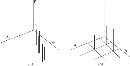
Figure 3.13 (a) A data set with multicollinearity. (b) Orthogonal regressors.

3.11 WHY DO REGRESSION COEFFICIENTS HAVE THE WRONG SIGN?

When using multiple regression, occasionally we find an apparent contradiction of intuition or theory when one or more of the regression coefficients seem to have the wrong sign. For example, the problem situation may imply that a particular regression coefficient should be positive, while the actual estimate of the parameter is negative. This “wrong”-sign problem can be disconcerting, as it is usually difficult to explain a negative estimate (say) of a parameter to the model user when that user believes that the coefficient should be positive. Mullet [1976] points out that regression coefficients may have the wrong sign for the following reasons:

1. The range of some of the regressors is too small.
2. Important regressors have not been included in the model.
3. Multicollinearity is present.
4. Computational errors have been made.

It is easy to see how the range of the x's can affect the sign of the regression coefficients. Consider the simple linear regression model. The variance of the regression coefficient is . Note that the variance of is inversely proportional to the “spread” of the regressor. Therefore, if the levels of x are all close together, the variance of will be relatively large. In some cases the variance of could be so large that a negative estimate (for example) of a regression coefficient that is really positive results. The situation is illustrated in Figure 3.14, which plots the sampling distribution of . Examining this figure, we see that the probability of obtaining a negative estimate of depends on how close the true regression coefficient is to zero and the variance of , which is greatly influenced by the spread of the x's.

In some situations the analyst can control the levels of the regressors. Although it is possible in these cases to decrease the variance of the regression coefficients by increasing the range of the x's, it may not be desirable to spread the levels of the regressors out too far. If the x's cover too large a range and the true response function is nonlinear, the analyst may have to develop a much more complex equation to adequately model the curvature in the system. Furthermore, many problems involve a region of x space of specific interest to the experimenter, and spreading the regressors out beyond this region of interest may be impractical or impossible. In general, we must trade off the precision of estimation, the likely complexity of the model, and the values of the regressors of practical interest when deciding how far to spread out the x's.

Figure 3.14 Sampling distribution of .

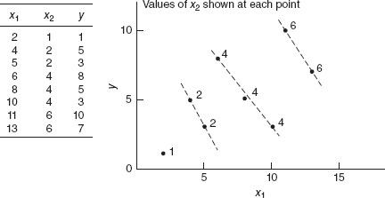
Figure 3.15 Plot of y versus x₁.

Wrong signs can also occur when important regressors have been left out of the model. In these cases the sign is not really wrong. The partial nature of the regression coefficients cause the sign reversal. To illustrate, consider the data in Figure 3.15.

Suppose we fit a model involving only y and x₁. The equation is

where = 0.463 is a “total” regression coefficient. That is, it measures the total effect of x₁ ignoring the information content in x₂. The model involving both x₁ and x₂ is

Note that now = −1.222, and a sign reversal has occurred. The reason is that = −1.222 in the multiple regression model is a partial regression coefficient; it measures the effect of x₁ given that x₂ is also in the model.

The data from this example are plotted in Figure 3.15. The reason for the difference in sign between the partial and total regression coefficients is obvious from inspection of this figure. If we ignore the x₂ values, the apparent relationship between y and x₁ has a positive slope. However, if we consider the relationship between y and x₁ for constant values of x₂, we note that this relationship really has a negative slope. Thus, a wrong sign in a regression model may indicate that important regressors are missing. If the analyst can identify these regressors and include them in the model, then the wrong signs may disappear.

Multicollinearity can cause wrong signs for regression coefficients. In effect, severe multicollinearity inflates the variances of the regression coefficients, and this increases the probability that one or more regression coefficients will have the wrong sign. Methods for diagnosing and dealing with multicollinearity are summarized in Chapter 9.

Computational error is also a source of wrong signs in regression models. Different computer programs handle round-off or truncation problems in different ways, and some programs are more effective than others in this regard. Severe multicollinearity causes the X′X matrix to be ill-conditioned, which is also a source of computational error. Computational error can cause not only sign reversals but regression coefficients to differ by several orders of magnitude. The accuracy of the computer code should be investigated when wrong-sign problems are suspected.

PROBLEMS

3.1 Consider the National Football League data in Table B.1.

1. Fit a multiple linear regression model relating the number of games won to the team's passing yardage (x₂), the percentage of rushing plays (x₇), and the opponents'yards rushing (x₈).
2. Construct the analysis-of-variance table and test for significance of regression.
3. Calculate t statistics for testing the hypotheses H₀: β₂ = 0 H₀: β₇ = 0, and H₀: β₈ = 0. What conclusions can you draw about the roles the variables x₂, x₇, and x₈ play in the model?
4. Calculate R² and R²_Adj for this model.
5. Using the partial F test, determine the contribution of x₇ to the model. How is this partial F statistic related to the t test for β₇ calculated in part c above?

3.2 Using the results of Problem 3.1, show numerically that the square of the simple correlation coefficient between the observed values y_i and the fitted values ŷ_i equals R².

3.3 Refer to Problem 3.1.

1. Find a 95% CI on β₇.
2. Find a 95% CI on the mean number of games won by a team when x₂ = 2300, x₇ = 56.0, and x₈ = 2100.

3.4 Reconsider the National Football League data from Problem 3.1. Fit a model to these data using only x₇ and x₈ as the regressors.

1. Test for significance of regression.
2. Calculate R² and R²_Adj. How do these quantities compare to the values computed for the model in Problem 3.1, which included an additional regressor (x₂)?
3. Calculate a 95% CI on β₇. Also find a 95% CI on the mean number of games won by a team when x₇ = 56.0 and x₈ = 2100. Compare the lengths of these CIs to the lengths of the corresponding CIs from Problem 3.3.
4. What conclusions can you draw from this problem about the consequences of omitting an important regressor from a model?

3.5 Consider the gasoline mileage data in Table B.3.

1. Fit a multiple linear regression model relatmg gasoline mileage y (miles per gallon) to engine displacement x₁ and the number of carburetor barrels x₆.
2. Construct the analysis-of-variance table and test for significance of regression.
3. Calculate R² and R²_Adj for this model. Compare this to the R² and the R²_Adj for the simple linear regression model relating mileage to engine displacement in Problem 2.4.
4. Find a 95% CI for β₁.
5. Compute the t statistics for testing H₀: β₁ = 0 and H₀: β₆ = 0. What conclusions can you draw?
6. Find a 95% CI on the mean gasoline mileage when x₁ = 275 in.³ and x₆ = 2 barrels.
7. Find a 95% prediction interval for a new observation on gasoline mileage when x₁ = 257 in.³ and x₆ = 2 barrels.

3.6 In Problem 2.4 you were asked to compute a 95% CI on mean gasoline prediction interval on mileage when the engine displacement x₁ = 275 in.³ Compare the lengths of these intervals to the lengths of the confidence and prediction intervals from Problem 3.5 above. Does this tell you anything about the benefits of adding x₆ to the model?

3.7 Consider the house price data in Table B.4.

1. Fit a multiple regression model relating selling price to all nine regressors.
2. Test for significance of regression. What conclusions can you draw?
3. Use t tests to assess the contribution of each regressor to the model. Discuss your findings.
4. What is the contribution of lot size and living space to the model given that all of the other regressors are included?
5. Is multicollinearity a potential problem in this model?

3.8 The data in Table B.5 present the performance of a chemical process as a function of sever controllable process variables.

1. Fit a multiple regression model relating CO₂ product (y) to total solvent (x₆) and hydrogen consumption (x₇).
2. Test for significance of regression. Calculate R² and R²_Adj.
3. Using t tests determine the contribution of x₆ and x₇ to the model.
4. Construct 95% CIs on β₆ and β₇.
5. Refitthe model using only x₆ as the regressor. Test for significance of regression and calculate R² and R²_Adj. Discuss your findings. Based on these statistics, are you satisfied with this model?
6. Construct a 95% CI on β₆ using the model you fit in part e. Compare the length of this CI to the length of the CI in part d. Does this tell you anything important about the contribution of x₇ to the model?
7. Compare the values of MS_Res obtained for the two models you have fit (parts a and e). How did the MS_Res change when you removed x₇ from the model? Does this tell you anything importaut about the contributiou of x₇ to the model?

3.9 The concentration of NbOCl₃ in a tube-flow reactor as a function of several controllable variables is shown in Table B.6.

1. Fit a multiple regression model relating concentration of NbOCl₃ (y) to concentration of COCl₂, (x₁) and mole fraction (x₄).
2. Test for significance of regression.
3. Calculate R² and R²_Adj for this model.
4. Using t tests, determine the contribution of x₁ and x₄ to the model. Are both regressors x₁ and x₄ necessary?
5. Is multicollinearity a potential concern in this model?

3.10 The quality of Pinot Noir wine is thought to be related to the properties of clarity, aroma, body, flavor, and oakiness. Data for 38 wines are given in Table B.11.

1. Fit a multiple linear regression model relating wine quality to these regressors.
2. Test for significance of regression. What conclusions can you draw?
3. Use t tests to assess the contribution of each regressor to the model. Discuss your findings.
4. Calculate R² and R²_Adj for this model. Compare these values to the R² and R²_Adj for the linear regression model relating wine quality to aroma and flavor. Discuss your results.
5. Find a 95 % CI for the regression coefficient for flavor for both models in part d. Discuss any differences.

3.11 An engineer performed an experiment to determine the effect of CO₂ pressure, CO₂ temperature, peanut moisture, CO₂ flow rate, and peanut particle size on the total yield of oil per batch of peanuts. Table B.7 summarizes the experimental results.

1. Fit a multiple linear regression model relating yield to these regressors.
2. Test for significance of regression. What conclusions can you draw?
3. Use t tests to assess the contribution of each regressor to the model. Discuss your findings
4. Calculate R² and R²_Adj for this model. Compare these values to the R² and R²_Adj for the multiple linear regression model relating yield to temperature and particle size. Discuss your results.
5. Find a 95% CI for the regression coefficient for temperature for both models in part d. Discuss any differences.

3.12 A chemical engineer studied the effect of the amount of surfactant and time on clathrate formation. Clathrates are used as cool storage media. Table B.8 summarizes the experimental results.

1. Fit a multiple linear regression model relating clathrate formation to these regressors.
2. Test for significance of regression. What conclusions can you draw?
3. Use t tests to assess the contribution of each regressor to the model. Discuss your findings.
4. Calculate R² and R²_Adj for this model. Compare these values to the R² and R²_Adj for the simple linear regression model relating clathrate formation to time. Discuss your results.
5. Find a 95% CI for the regression coefficient for time for both models in part d. Discuss any differences.

3.13 An engineer studied the effect of four variables on a dimensionless factor used to describe pressure drops in a screen-plate bubble column. Table B.9 summarizes the experimental results.

1. Fit a multiple linear regression model relating this dimensionless number to these regressors.
2. Test for significance of regression. What conclusions can you draw?
3. Use t tests to assess the contribution of each regressor to the model. Discuss your findings.
4. Calculate R² and R²_Adj for this model. Compare these values to the R² and R²_Adj for the multiple linear regression model relating the dimensionless number to x₂ and x₃. Discuss your results.
5. Find a 99% CI for the regression coefficient for x₂ for both models in part d. Discuss any differences.

3.14 The kinematic viscosity of a certain solvent system depends on the ratio of the two solvents and the temperature. Table B.10 summarizes a set of experimental results.

1. Fit a multiple linear regression model relating the viscosity to the two regressors.
2. Test for significance of regression. What conclusions can you draw?
3. Use t tests to assess the contribution of each regressor to the model. Discuss your findings.
4. Calculate R² and R²_Adj for this model. Compare these values to the R² and R²_Adj for the simple linear regression model relating the viscosity to temperature only. Discuss your results.
5. Find a 99% CI for the regression coefficient for temperature for both models in part d. Discuss any differences.

3.15 McDonald and Ayers [1978] present data from an early study that examined the possible link between air pollution and mortality. Table B.15 summarizes the data. The response MORT is the total age-adjusted mortality from all causes, in deaths per 100,000 population. The regressor PRECIP is the mean annual precipitation· (in inches), EDUC is the median number of school years completed for persons of age 25 years or older, NONWHITE is the percentage of the 1960 population that is nonwhite, NOX is the relative pollution potential of oxides of nitrogen, and SO₂ is the relative pollution potential of sulfur dioxide. “Relative pollution potential” is the product of the tons emitted per day per square kilometer and a factor correcting the SMSA dimensions and exposure.

1. Fit a multiple linear regression model relating the mortality rate to these regressors.
2. Test for significance of regression. What conclusions can you draw?
3. Use t tests to assess the contribution of each regressor to the model. Discuss your findings.
4. Calculate R² and R²_Adj for this model.
5. Find a 95% CI for the regression coefficient for SO₂.

3.16 Rossman [1994] presents an interesting study of average life expectancy of 40 countries. Table B.16 gives the data. The study has three responses: LifeExp is the overall average life expectancy. LifeExpMale is the average life expectancy for males, and LifeExpFemale is the average life expectancy for females. The regressors are People-per-TV, which is the average number of people per television, and People-per-Dr, which is the average number of people per physician.

1. Fit different multiple linear regression models for each response.
2. Test each model for significance of regression. What conclusions can you draw?
3. Use t tests to assess the contribution of each regressor to each model. Discuss your findings.
4. Calculate R² and R²_Adj for each model.
5. Find a 95% CI for the regression coefficient for People-per-Dr in each model.

3.17 Consider the patient satisfaction data in Table B.17. For the purposes of this exercise, ignore the regressor “Medical-Surgical.” Perform a thorough analysis of these data. Please discuss any differences from the analyses outlined in Sections 2.7 and 3.6.

3.18 Consider the fuel consumption data in Table B.18. For the purposes of this exercise, ignore regressor x₁. Perform a thorough analysis of these data. What conclusions do you draw from this analysis?

3.19 Consider the wine quality of young red wines data in Table B.19. For the purposes of this exercise, ignore regressor x₁. Perform a thorough analysis of these data. What conclusions do you draw from this analysis?

3.20 Consider the methanol oxidation data in Table B.20. Perform a thorough analysis of these data. What conclusions do you draw from this analysis?

3.21 A chemical engineer is investigating how the amount of conversion of a product from a raw material (y) depends on reaction temperature (x₁) and reaction time (x₂). He has developed the following regression models:

1. ŷ=100 + 0.2x₁ + 4x₂
2. ŷ= 95 + 0.15x₁ + 3x₂ + 1x₁x₂

Both ]models have been built over the range 20 ≤ x₁ ≤ 50 (°C) and 0.5 ≤ x₂ ≤ 10 (hours).

1. Using both models, what is the predicted value of conversion when x₂ = 2 in terms of x₁? Repeat this calculation for x₂ = 8. Draw a graph of the predicted values as a function of temperature for both conversion models. Comment on the effect of the interaction term in model 2.
2. Find the expected change in the mean conversion for a unit change in temperature x₁ for model 1 when x₂ = 5. Does this quantity depend on the specific value of reaction time selected? Why?
3. Find the expected change in the mean conversion for a unit change in temperature x₁ for model 2 when x₂ = 5. Repeat this calculation for x₂ = 2 and x₂ = 8. Does the result depend on the value selected for x₂? Why?

3.22 Show that an equivalent way to perform the test for significance of regression in multiple linear regression is to base the test on R² as follows: To test H₀: β₁ = β₂ = … = β_k versus H₁: at least one β_j ≠ 0, calculate

and to reject H₀ if the computed value of F₀ exceeds F_α,k,n−p, where p = k + 1

3.23 Suppose that a linear regression model with k = 2 regressors has been fit to n = 25 observations and R² = 0.90.

1. Test for significance of regression at α = 0.05. Use the results of the previous problem.
2. What is the smallest value of R² that would lead to the conclusion of a significant regression if α = 0.05? Are you surprised at how small this value of R² is?

3.24 Show that an alternate computing formula for the regression sum of squares in a linear regression model is

3.25 Consider the multiple linear regression model

Using the procedure for testing a general linear hypothesis, show how to test

3.26 Suppose that we have two independent samples, say

Two models can be fit to these samples,

1. Show how these two separate models can be written as a single model.
2. Using the result in part a, show how the general linear hypothesis can be used to test the equality of slopes β₁ and γ₁.
3. Using the result in part a, show how the general linear hypothesis can be used to test the equality of the two regression lines.
4. Using the result in part a, show how the general linear hypothesis can be used to test that both slopes are equal to a constant c.

3.27 Show that Var(ŷ) = σ²H.

3.28 Prove that the matrices H and I − H are idempotent, that is, HH = H and (I − H)(I − H) = I − H.

3.29 For the simple linear regression model, show that the elements of the hat matrix are

Discuss the behavior of these quantities as x_i moves farther from ,

3.30 Consider the multiple linear regression model y = Xβ + ε. Show that the least-squares estimator can be written as

3.31 Show that the residuals from a linear regression model can be expressed as e = (I − H)ε. [Hint: Refer to Eq. (3.15b).]

3.32 For the multiple linear regression model, show that SS_R(β) = y′Hy.

3.33 Prove that R² is the square of the correlation between y and ŷ.

3.34 Constrained least squares. Suppose we wish to find the least-squares estimator of β in the model y = Xβ + ε subject to a set of equality constraints on β, say Tβ = c. Show that the estimator is

where . Discuss situations in which this constrained estimator might be appropriate. Find the residual sum of squares for the constrained estimator. Is it larger or smaller than the residual sum of squares in the unconstrained case?

3.35 Let x_j be the jth row of X, and X_-j be the X matrix with the jth row removed. Show that

3.36 Consider the following two models where E(ε) = 0 and Var(ε) = σ²I:

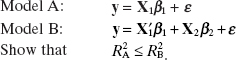
3.37 Suppose we fit the model y = X₁β₂ + ε when the true model is actually given by y = X₁β₂ + X₂β₂ + ε. For both models, assume E(ε) = 0 and Var(ε) = σ²I. Find the expected value and variance of the ordinary least-squares estimate, . Under what conditions is this estimate unbiased?

3.38 Consider a correctly specified regression model with p terms, including the intercept. Make the usual assumptions about ε. Prove that

3.39 Let R²_j be the coefficient of determination when we regress the jth regressor on the other k − 1 regressors. Show that the jth variance inflation factor may be expressed as

3.40 Consider the hypotheses for the general linear model, which are of the form

where T is a q × p matrix of rank q. Derive the appropriate F statistic under both the null and alternative hypothesis.