
CHAPTER 13
GENERALIZED LINEAR MODELS
13.1 INTRODUCTION
In Chapter 5, we developed and illustrated data transformation as an approach to fitting regression models when the assumptions of a normally distributed response variable with constant variance are not appropriate. Transformation of the response variable is often a very effective way to deal with both response nonnormality and inequality of variance. Weighted least squares is also a potentially useful way to handle the non-constant variance problem. In this chapter, we present an alternative approach to data transformation when the “usual” assumptions of normality and constant variance are not satisfied. This approach is based on the generalized linear model (GLM).
The GLM is a unification of both linear and nonlinear regression models that also allows the incorporation of nonnormal response distributions. In a GLM, the response variable distribution must only be a member of the exponential family, which includes the normal, Poisson, binomial, exponential, and gamma distributions as members. Furthermore, the normal-error linear model is just a special case of the GLM, so in many ways, the GLM can be thought of as a unifying approach to many aspects of empirical modeling and data analysis.
We begin our presentation of these models by considering the case of logistic regression. This is a situation where the response variable has only two possible outcomes, generically called success and failure and denoted by 0 and 1. Notice that the response is essentially qualitative, since the designation success or failure is entirely arbitrary. Then we consider the situation where the response variable is a count, such as the number of defects in a unit of product or the number of relatively rare events such as the number of Atlantic hurricanes that make landfall on the United States in a year. Finally, we discuss how all these situations are unified by the GLM. For more details of the GLM, refer to Myers, Montgomery, Vining, and Robinson [2010].
13.2 LOGISTIC REGRESSION MODELS
13.2.1 Models with a Binary Response Variable
Consider the situation where the response variable in a regression problem takes on only two possible values, 0 and 1. These could be arbitrary assignments resulting from observing a qualitative response. For example, the response could be the outcome of a functional electrical test on a semiconductor device for which the results are either a success, which means the device works properly, or a failure, which could be due to a short, an open, or some other functional problem.
Suppose that the model has the form
where x′i = [1, xi1, xi2, …, xik], β′ = [β0, β1, β2, …, βk], and the response variable yj, takes on the value either 0 or 1. We will assume that the response variable yi is a Bernoulli random variable with probability distribution as follows:
| yi | Probability |
| 1 | P(yi = 1) = πi |
| 0 | P(yi = 0) = 1 − πi |
Now since E(εi) = 0, the expected value of the response variable is
![]()
This implies that
![]()
This means that the expected response given by the response function E(ii) = x′iβ is just the probability that the response variable takes on the value 1.
There are some very basic problems with the regression model in Eq. (13.1). First, note that if the response is binary, then the error terms ?i can only take on two values, namely,

Consequently, the errors in this model cannot possibly be normal. Second, the error variance is not constant, since
![]()
Notice that this last expression is just
![]()
since E(yi) = x′iβ = πi. This indicates that the variance of the observations (which is the same as the variance of the errors because εi = yi − πi, and πi is a constant) is a function of the mean. Finally, there is a constraint on the response function, because
![]()
This restriction can cause serious problems with the choice of a linear response function, as we have initially assumed in Eq. (13.1) It would be possible to fit a model to the data for which the predicted values of the response lie outside the 0, 1 interval.
Generally, when the response variable is binary, there is considerable empirical evidence indicating that the shape of the response function should be nonlinear. A monotonically increasing (or decreasing) S-shaped (or reverse S-shaped) function, such as shown in Figure 13.1, is usually employed. This function is called the logistic response function and has the form
The logistic response function can be easily linearized. One approach defines the structural portion of the model in terms of a function of the response function mean. Let
be the linear predictor where η is defined by the transformation
This transformation is often called the logit transformation of the probability π, and the ratio π/(1 − π) in the transformation is called the odds. Sometimes the logit transformation is called the log-odds.
13.2.2 Estimating the Parameters in a Logistic Regression Model
The general form of the logistic regression model is

Figure 13.1 Examples of the logistic response function: (a) E (y) = 1/(1 + e−6.0 + 1.0x);(b) E (y) = 1/(1 + e−6.0 + 1.0x); (c) E(y) = 1/(1+e−5.0+0.65x1+0.4x2); (d) E(y) = 1/(1+e−5.0+0.65x1+0.4x2+0.15x1x2).
where the observations yi are independent Bernoulli random variables with expected values
We use the method of maximum likelihood to estimate the parameters in the linear predictor x′iβ.
Each sample observation follows the Bernoulli distribution, so the probability distribution of each sample observation is
![]()
and of course each observation yi takes on the value 0 or 1. Since the observations are independent, the likelihood function is just
It is more convenient to work with the log-likelihood

Now since 1 − πi = [1 + exp(x′iβ)]−1 and ηi = in[πi/(1 − πi)] = x′iβ the log-likelihood can be written as
Often in logistic regression models we have repeated observations or trials at each level of the x variables. This happens frequently in designed experiments. Let yi represent the number of 1's observed for the ith observation and ni be the number of trials at each observation. Then the log-likelihood becomes

Numerical search methods could be used to compute the maximum-likelihood estimates (or MLEs) ![]() . However, it turns out that we can use iteratively reweighted least squares (IRLS) to actually find the MLEs. For details of this procedure, refer to Appendix C.14. There are several excellent computer programs that implement maximum-likelihood estimation for the logistic regression model, such as SAS PROC GENMOD, JMP and Minitab.
. However, it turns out that we can use iteratively reweighted least squares (IRLS) to actually find the MLEs. For details of this procedure, refer to Appendix C.14. There are several excellent computer programs that implement maximum-likelihood estimation for the logistic regression model, such as SAS PROC GENMOD, JMP and Minitab.
Let ![]() be the final estimate of the model parameters that the above algorithm produces. If the model assumptions are correct, then we can show that asymptotically
be the final estimate of the model parameters that the above algorithm produces. If the model assumptions are correct, then we can show that asymptotically
where the matrix V is an n × n diagonal matrix containing the estimated variance of each observation on the main diagonal; that is, the ith diagonal element of V is
![]()
The estimated value of the linear predictor is ![]() , and the fitted value of the logistic regression model is written as
, and the fitted value of the logistic regression model is written as

Example 13.1 The Pneumoconiosis Data
A 1959 article in the journal Biometrics presents data concerning the proportion of coal miners who exhibit symptoms of severe pneumoconiosis and the number of years of exposure. The data are shown in Table 13.1. The response variable of interest, y, is the proportion of miners who have severe symptoms. A graph of the response variable versus the number of years of exposure is shown in Figure 13.2. A reasonable probability model for the number of severe cases is the binomial, so we will fit a logistic regression model to the data.
Table 13.2 contains some of the output from Minitab. In subsequent sections, we will discuss in more detail the information contained in this output. The section of the output entitled Logistic Regression Table presents the estimates of the regression coefficients in the linear predictor.
The fitted logistic regression model is
![]()
where x is the number of years of exposure. Figure 13.3 presents a plot of the fitted values from this model superimposed on the scatter diagram of the sample data. The logistic regression model seems to provide a reasonable fit to the sample data. If we let CASES be the number of severe cases and MINERS be the number of miners the appropriate SAS code to analyze these data is
proc genmod;
model CASES = MINERS / dist = binomial type1 type3;
Minitab will also calculate and display the covariance matrix of the model parameters. For the model of the pneumoconiosis data, the covariance matrix is
![]()
The standard errors of the model parameter estimates reported in Table 13.2 are the square roots of the main diagonal elements of this matrix.
TABLE 13.1 The Pneumoconiosis Data
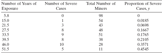

Figure 13.2 A scatter diagram of the pneumoconiosis data from Table 13.1.

Figure 13.3 The fitted logistic regression model for pneumoconiosis data from Table 13.1.
TABLE 13.2 Binary Logistic Regression: Severe Cases, Number of Miners versus Years

13.2.3 Interpretation of the Parameters in a Logistic Regression Model
It is relatively easy to interpret the parameters in a logistic regression model. Consider first the case where the linear predictor has only a single regressor, so that the fitted value of the linear predictor at a particular value of x, say xi, is
![]()
The fitted value at xi + 1 is
![]()
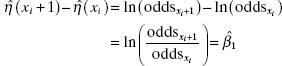
and the difference in the two predicted values is
![]()
Now ![]() is just the log-odds when the regressor variable is equal to xi, and
is just the log-odds when the regressor variable is equal to xi, and ![]() is just the log-odds when the regressor is equal to xi + 1. Therefore, the difference in the two fitted values is
is just the log-odds when the regressor is equal to xi + 1. Therefore, the difference in the two fitted values is
If we take antilogs, we obtain the odds ratio
The odds ratio can be interpreted as the estimated increase in the probability of success associated with a one-unit change in the value of the predictor variable. In general, the estimated increase in the odds ratio associated with a change of d units in the predictor variable is ![]() .
.
Example 13.2 The Pneumoconiosis Data
In Example 13.1 we fit the logistic regression model
![]()
to the pneumoconiosis data of Table 13.1. Since the linear predictor contains only one regressor variable and ![]() , we can compute the odds ratio from Eq. (13.12) as
, we can compute the odds ratio from Eq. (13.12) as
![]()
This implies that every additional year of exposure increases the odds of contracting a severe case of pneumoconiosis by 10%. If the exposure time increases by 10 years, then the odds ratio becomes ![]() . This indicates that the odds more than double with a 10-year exposure.
. This indicates that the odds more than double with a 10-year exposure.
There is a close connection between the odds ratio in logistic regression and the 2 × 2 contingency table that is widely used in the analysis of categorical data. Consider Table 13.3 which presents a 2 × 2 contingency table where the categorical response variable represents the outcome (infected, not infected) for a group of patients treated with either an active drug or a placebo. The nij are the numbers of patients in each cell. The odds ratio in the 2 × 2 contingency table is defined as
![]()
Consider a logistic regression model for these data. The linear predictor is
![]()
When x1 = 0, we have
![]()
Now let x1 = 1:
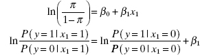
Solving for β1 yields
![]()
TABLE 13.3 A 2 × 2 Contingency Table

so exp(β1) is equivalent to the odds ratio in the 2 × 2 contingency table. However, the odds ratio from logistic regression is much more general than the traditional 2 × 2 contingency table odds ratio. Logistic regression can incorporate other predictor variables, and the presence of these variables can impact the odds ratio. For example, suppose that another variable, x2 = age, is available for each patient in the drug study depicted in Table 13.3. Now the linear predictor for the logistic regression model for the data would be
![]()
This model allows the predictor variable age to impact the estimate of the odds ratio for the drug variable. The drug odds ratio is still exp(β1), but the estimate of β1 is potentially affected by the inclusion of x2 = age in the model. It would also be possible to include an interaction term between drug and age in the model, say
![]()
In this model the odds ratio for drug depends on the level of age and would be computed as exp(β1 + β12x2).
The interpretation of the regression coefficients in the multiple logistic regression model is similar to that for the case where the linear predictor contains only one regressor. That is, the quantity ![]() is the odds ratio for regressor xj, assuming that all other predictor variables are constant.
is the odds ratio for regressor xj, assuming that all other predictor variables are constant.
13.2.4 Statistical Inference on Model Parameters
Statistical inference in logistic regression is based on certain properties of maximum-likelihood estimators and on likelihood ratio tests. These are large-sample or asymptotic results. This section discusses and illustrates these procedures using the logistic regression model fit to the pneumoconiosis data from Example 13.1.
Likelihood Ratio Tests A likelihood ratio test can be used to compare a “full” model with a “reduced” model that is of interest. This is analogous to the “extra-sum-of-squares” technique that we have used previously to compare full and reduced models. The likelihood ratio test procedure compares twice the logarithm of the value of the likelihood function for the full model (FM) to twice the logarithm of the value of the likelihood function of the reduced model (RM) to obtain a test statistic, say
For large samples, when the reduced model is correct, the test statistic LR follows a chi-square distribution with degrees of freedom equal to the difference in the number of parameters between the full and reduced models. Therefore, if the test statistic LR exceeds the upper α percentage point of this chi-square distribution, we would reject the claim that the reduced model is appropriate.
The likelihood ratio approach can be used to provide a test for significance of regression in logistic regression. This test uses the current model that had been fit to the data as the full model and compares it to a reduced model that has constant probability of success. This constant-probability-of-success model is
![]()
that is, a logistic regression model with no regressor variables. The maximum-likelihood estimate of the constant probability of success is just y/n, where y is the total number of successes that have been observed and n is the number of observations. Substituting this into the log-likelihood function in Equation (13.9) gives the maximum value of the log-likelihood function for the reduced model as
![]()
Therefore the likelihood ratio test statistic for testing significance of regression is

A large value of this test statistic would indicate that at least one of the regressor variables in the logistic regression model is important because it has a nonzero regression coefficient.
Minitab computes the likelihood ratio test for significance of regression in logistic regression. In the Minitab output in Table 13.2 the test statistic in Eq. (13.14) is reported as G = 50.852 with one degree of freedom (because the full model has only one predictor). The reported P value is 0.000 (the default reported by Minitab when the calculated P value is less than 0.001).
Testing Goodness of Fit The goodness of fit of the logistic regression model can also be assessed using a likelihood ratio test procedure. This test compares the current model to a saturated model, where each observation (or group of observations when ni < 1) is allowed to have its own parameter (that is, a success probability). These parameters or success probabilities are yi/ni, where yi is the number of successes and ni is the number of observations. The deviance is defined as twice the difference in log-likelihoods between this saturated model and the full model (which is the current model) that has been fit to the data with estimated success probability ![]() . The deviance is defined as
. The deviance is defined as
In calculating the deviance, note that ![]() if y = 0, and if y = n we have
if y = 0, and if y = n we have ![]() . When the logistic regression model is an adequate fit to the data and the sample size is large, the deviance has a chi-square distribution with n − p degrees of freedom, where p is the number of parameters in the model. Small values of the deviance (or a large P value) imply that the model provides a satisfactory fit to the data, while large values of the deviance imply that the current model is not adequate. A good rule of thumb is to divide the deviance by its number of degrees of freedom. If the ratio D/(n − p) is much greater than unity, the current model is not an adequate fit to the data.
. When the logistic regression model is an adequate fit to the data and the sample size is large, the deviance has a chi-square distribution with n − p degrees of freedom, where p is the number of parameters in the model. Small values of the deviance (or a large P value) imply that the model provides a satisfactory fit to the data, while large values of the deviance imply that the current model is not adequate. A good rule of thumb is to divide the deviance by its number of degrees of freedom. If the ratio D/(n − p) is much greater than unity, the current model is not an adequate fit to the data.
Minitab calculates the deviance goodness-of-fit statistic. In the Minitab output in Table 13.2, the deviance is reported under Goodness-of-Fit Tests. The value reported is D = 6.05077 with n − p = 8 − 2 = 6 degrees of freedom. The P value iis 0.418 and the ratio D/(n − p) is approximately unity, so there is no apparent reason to doubt the adequacy of the fit.
The deviance has an analog in ordinary normal-theory linear regression. In the linear regression model D = SSRes/σ2. This quantity has a chi-square distribution with n − p degrees of freedom if the observations are normally and independently distributed. However, the deviance in normal-theory linear regression contains the unknown nuisance parameter σ2, so we cannot compute it directly. However, despite this small difference, the deviance and the residual sum of squares are essentially equivalent.
Goodness of fit can also be assessed with a Pearson chi-square statistic that compares the observed and expected probabilities of success and failure at each group of observations. The expected number of successes is ![]() and the expected number of failures is
and the expected number of failures is ![]() . The Pearson chi-square statistic is
. The Pearson chi-square statistic is
The Pearson chi-square goodness-of-fit statistic can be compared to a chi-square distribution with n − p degrees of freedom. Small values of the statistic (or a large P value) imply that the model provides a satisfactory fit to the data. The Pearson chi-square statistic can also be divided by the number of degrees of freedom n − p and the ratio compared to unity. If the ratio greatly exceeds unity, the goodness of fit of the model is questionable.
The Minitab output in Table 13.2 reports the Pearson chi-square statistic under Goodness-of-Fit Tests. The value reported is χ2 = 6.02854 with n − p = 8 − 2 = 6 degrees of freedom. The P value is 0.540 and the ratio D/(n − p) does not exceed unity, so there is no apparent reason to doubt the adequacy of the fit.
When there are no replicates on the regressor variables, the observations can be grouped to perform a goodness-of-fit test called the Hosmer-Lemeshow test. In this procedure the observations are classified into g groups based on the estimated probabilities of success. Generally, about 10 groups are used (when g = 10 the groups are called the deciles of risk) and the observed number of successes Oj and failures Nj − Oj are compared with the expected frequencies in each group, ![]() and
and ![]() , where Nj is the number of observations in the jth group and the average estimated success probability in the jth group is
, where Nj is the number of observations in the jth group and the average estimated success probability in the jth group is ![]() . The Hosmer–Lemeshow statistic is really just a Pearson chi-square goodness-of-fit statistic comparing observed and expected frequencie:
. The Hosmer–Lemeshow statistic is really just a Pearson chi-square goodness-of-fit statistic comparing observed and expected frequencie:
If the fitted logistic regression model is correct, the HL statistic follows a chi-square distribution with g − 2 degrees of freedom when the sample size is large. Large values of the HL statistic imply that the model is not an adequate fit to the data. It is also useful to compute the ratio of the Hosmer–Lemeshow statistic to the number of degrees of freedom g − p with values close to unity implying an adequate fit.
MINlTAB computes the Hosmer–Lemeshow statistic. For the pneumoconiosis data the HL statistic is reported in Table 13.2 under Goodness-of-Fit Tests. This computer package has combined the data into g = 7 groups. The grouping and calculation of observed and expected frequencies for success and failure are reported at the bottom of the MINlTAB output. The value of the test statistic is HL = 5.00360 with g − p = 7 − 2 = 5 degrees of freedom. The P value is 0.415 and the ratio HL/df is very close to unity, so there is no apparent reason to doubt the adequacy of the fit.
Testing Hypotheses on Subsets of Parameters Using Deviance We can also use the deviance to test hypotheses on subsets of the model parameters, just as we used the difference in regression (or error) sums of squares to test similar hypotheses in the normal-error linear regression model case. Recall that the model can be written as
where the full model has p parameters, β1 contains p − r of these parameters, β2 contains r of these parameters, and the columns of the matrices X1 and X2 contain the variables associated with these parameters.
The deviance of the full model will be denoted by D(β). Suppose that we wish to test the hypotheses
Therefore, the reduced model is
Now fit the reduced model, and let D(β1) be the deviance for the reduced model. The deviance for the reduced model will always be larger than the deviance for the full model, because the reduced model contains fewer parameters. However, if the deviance for the reduced model is not much larger than the deviance for the full model, it indicates that the reduced model is about as good a fit as the full model, so it is likely that the parameters in β2 are equal to zero. That is, we cannot reject the null hypothesis above. However, if the difference in deviance is large, at least one of the parameters in β2 is likely not zero, and we should reject the null hypothesis. Formally, the difference in deviance is
and this quantity has n − (p − r) − (n − p) = r degrees of freedom. If the null hypothesis is true and if n is large, the difference in deviance in Eq. (13.21) has a chi-square distribution with r degrees of freedom. Therefore, the test statistic and decision criteria are
Sometimes the difference in deviance D(β2|β1) is called the partial deviance.
Example 13.3 The Pneumoconiosis Data
Once again, reconsider the pneumoconiosis data of Table 13.1. The model we initially fit to the data is
![]()
Suppose that we wish to determine whether adding a quadratic term in the linear predictor would improve the model. Therefore, we will consider the full model to be
![]()
Table 13.4 contains the output from Minitab for this model. Now the linear predictor for the full model can be written as

TABLE 13.4 Binary Logistic Regression: Severe Cases, Number of Miners versus Years

From Table 13.4, we find that the deviance for the full model is
![]()
with n − p = 8 − 3 = 5 degrees of freedom. Now the reduced model has Xlβ1 = β0 + β1x, so X2β2 = β11x2 with r = 1 degree of freedom. The reduced model was originally fit in Example 13.1, and Table 13.2 shows the deviance for the reduced model to be
![]()
with p − r = 3 − 1 = 2 degrees of freedom. Therefore, the difference in deviance between the full and reduced models is computed using Eq. (13.21) as

which would be referred to a chi-square distribution with r = 1 degree of freedom. Since the P value associated with the difference in deviance is 0.0961, we might conclude that there is some marginal value in including the quadratic term in the regressor variable x = years of exposure in the linear predictor for the logistic regression model.
Tests on Individual Model Coefficients Tests on individual model coefficients, such as
![]()
can be conducted by using the difference-in-deviance method as illustrated in Example 13.3. There is another approach, also based on the theory of maximum likelihood estimators. For large samples, the distribution of a maximum-likelihood estimator is approximately normal with little or no bias. Furthermore, the variances and covariances of a set of maximum-likelihood estimators can be found from the second partial derivatives of the log-likelihood function with respect to the model parameters, evaluated at the maximum-likelihood estimates. Then a t-like statistic can be constructed to test the above hypotheses. This is sometimes referred to as Wald inference.
Let G denote the p × p matrix of second partial derivatives of the log-likelihood function, that is,
![]()
G is called the Hessian matrix. If the elements of the Hessian are evaluated at the maximum-likelihood estimators ![]() , the large-sample approximate covariance matrix of the regression coefficients is
, the large-sample approximate covariance matrix of the regression coefficients is
Notice that this is just the covariance matrix of ![]() given earlier. The square roots of the diagonal elements of this covariance matrix are the large-sample standard errors of the regression coefficients, so the test statistic for the null hypothesis in
given earlier. The square roots of the diagonal elements of this covariance matrix are the large-sample standard errors of the regression coefficients, so the test statistic for the null hypothesis in
![]()
is
The reference distribution for this statistic is the standard normal distribution. Some computer packages square the Z0 statistic and compare it to a chi-square distribution with one degree of freedom.
Example 13.4 The Pneumoconiosis Data
Table 13.3 contains output from MlNITAB for the pneumoconiosis data, originally given in Table 13.1. The fitted model is
![]()
The Minitab output gives the standard errors of each model coefficient and the Z0 test statistic in Eq. (13.24). Notice that the P value for β1 is P = 0.014, implying that years of exposure is an important regressor. However, notice that the P value for β1 is P = 0.127, suggesting that the squared term in years of exposure does not contribute significantly to the fit.
Recall from the previous example that when we tested for the significance of β11 using the partial deviance method we obtained a different P value. Now in linear regression, the t test on a single regressor is equivalent to the partial F test on a single variable (recall that the square of the t statistic is equal to the partial F statistic). However, this equivalence is only true for linear models, and the GLM is a nonlinear model.
Confidence Intervals It is straightforward to use Wald inference to construct confidence intervals in logistic regression. Consider first finding confidence intervals on individual regression coefficients in the linear predictor. An approximate 100(1 − α) percent confidence interval on the jth model coefficient is
Example 13.5 The Pneumoconiosis Data
Using the Minitab output in Table 13.3, we can find an approximate 95% confidence interval on β11 from Eq. (13.25) as follows:

Notice that the confidence interval includes zero, so at the 5% significance level, we would not reject the hypothesis that this model coefficient is zero. The regression coefficient βj is also the logarithm of the odds ratio. Because we know how to find a confidence interval (CI) for βj, it is easy to find a CI for the odds ratio. The point estimate of the odds ratio is ![]() and the 100(1 − α) percent CI for the odds ratio is
and the 100(1 − α) percent CI for the odds ratio is
The CI for the odds ratio is generally not symmetric around the point estimate. Furthermore, the point estimate ![]() actually estimates the median of the sampling distribution of
actually estimates the median of the sampling distribution of ![]() .
.
Example 13.6 The Pneumoconiosis Data
Reconsider the original logistic regression model that we fit to the pneumoconiosis data in Example 13.1. From the Minitab output for this data shown in Table 13.2 we find that the estimate of β1 is ![]() and the odds ratio
and the odds ratio ![]() . Because the standard error of
. Because the standard error of ![]() is se
is se![]() , we can find a 95% CI on the odds ratio as follows:
, we can find a 95% CI on the odds ratio as follows:
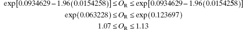
This agrees with the 95% CI reported by Minitab in Table 13.2.
It is possible to find a CI on the linear predictor at any set of values of the predictor variables that is of interest. Let x′0 = [1, x01, x02, …, x0k] be the values of the regressor variables that are of interest. The linear predictor evaluated at x0 is ![]() . The variance of the linear predictor at this point is
. The variance of the linear predictor at this point is
![]()
so the 100(1 − α) percent CI on the linear predictor is
The CI on the linear predictor given in Eq. (13.27) enables us to find a CI on the estimated probability of success π0 at the point of interest x′0 = [1, x01, x02, …, x0k]. Let
![]()
and
![]()
be the lower and upper 100(1 − α) percent confidence bounds on the linear predictor at the point x0 from Eq. (13.27). Then the point estimate of the probability of success at this point is ![]() and the 100(1 − α) percent CI on the probability of success at x0 is
and the 100(1 − α) percent CI on the probability of success at x0 is
Example 13.7 The Pneumoconiosis Data
Suppose that we want to find a 95% CI on the probability of miners with x = 40 years of exposure contracting pneumoconiosis. From the fitted logistic regression model in Example 13.1, we can calculate a point estimate of the probability at 40 years of exposure as
![]()
To find the CI, we need to calculate the variance of the linear predictor at this point. The variance is
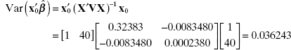
Now
![]()
and
![]()
Therefore the 95% CI on the estimated probability of contracting pneumoconiosis for miners that have 40 years of exposure is

13.2.5 Diagnostic Checking in Logistic Regression
Residuals can be used for diagnostic checking and investigating model adequacy in logistic regression. The ordinary residuals are defined as usual,
In linear regression the ordinary residuals are components of the residual sum of squares; that is, if the residuals are squared and summed, the residual sum of squares results. In logistic regression, the quantity analogous to the residual sum of squares is the deviance. This leads to a deviance residual, defined as
The sign of the deviance residual is the same as the sign of the corresponding ordinary residual. Also, when yi = 0, ![]() , and when yi = ni,
, and when yi = ni, ![]() . Similarly, we can define a Pearson residual
. Similarly, we can define a Pearson residual
It is also possible to define a hat matrix analog for logistic regression,
where V is the diagonal matrix defined earlier that has the variances of each observation on the main diagonal, ![]() , and these variances are calculated using the estimated probabilities that result from the fitted logistic regression model. The diagonal elements of H, hii, can be used to calculate a standardized Pearson residual
, and these variances are calculated using the estimated probabilities that result from the fitted logistic regression model. The diagonal elements of H, hii, can be used to calculate a standardized Pearson residual
The deviance and Pearson residuals are the most appropriate for conducting model adequacy checks. Plots of these residuals versus the estimated probability and a normal probability plot of the deviance residuals are useful in checking the fit of the model at individual data points and in checking for possible outliers.
TABLE 13.5 Residuals for the Pneumoconiosis Data


Figure 13.4 Normal probability plot of the deviance residuals.

Figure 13.5 Plot of deviance residuals versus estimated probabilities.
Table 13.5 displays the deviance residuals, Pearson residuals, hat matrix diagonals, and the standardized Pearson residuals for the pneumoconiosis data. To illustrate the calculations, consider the deviance residual for the third observation. From Eq. (13.30)
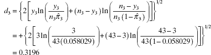
which closely matches the value reported by Minitab in Table 13.5. The sign of the deviance residual d3 is positive because the ordinary residual ![]() is positive.
is positive.
Figure 13.4 is the normal probability plot of the deviance residuals and Figure 13.5 plots the deviance residuals versus the estimated probability of success. Both plots indicate that there may be some problems with the model fit. The plot of deviance residuals versus the estimated probability indicates that the problems may be at low estimated probabilities. However, the number of distinct observations is small (n = 8), so we should not attempt to read too much into these plots.
13.2.6 Other Models for Binary Response Data
In our discussion of logistic regression we have focused on using the logit, defined as ln[π/(1 − π)], to force the estimated probabilities to lie between zero and unity. This leads to the logistic regression model
![]()
However, this is not the only way to model a binary response. Another possibility is to make use of the cumulative normal distribution, say Φ−1(π). The function Φ−1(π) is called the Probit. A linear predictor can be related to the probit, x′β = Φ−1(π), resulting in a regression model
Another possible model is provided by the complimentary log-log relationship log[−log(1 − π) = x′β. This leads to the regression model
A comparison of all three possible models for the linear predictor x′β = 1 + 5x is shown in Figure 13.6. The logit and probit functions are very similar, except when the estimated probabilities are very close to either 0 or 1. Both of these functions have estimated probability π = ½ when x = −β0/β1 and exhibit symmetric behavior around this value. The complimentary log-log function is not symmetric. In general, it is very difficult to see meaningful differences between these three models when sample sizes are small.
13.2.7 More Than Two Categorical Outcomes
Logistic regression considers the situation where the response variable is categorical, with only two outcomes. We can extend the classical logistic regression model to cases involving more than two categorical outcomes. First consider a case where there are m + 1 possible categorical outcomes but the outcomes are nominal. By this we mean that there is no natural ordering of the response categories. Let the outcomes be represented by 0, 1, 2, …, m. The probabilities that the responses on observation i take on one of the m + 1 possible outcomes can be modeled as
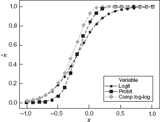
Figure 13.6 Logit, probit, and complimentary log-log functions for the linear predictor x′β = 1 + 5x.

Notice that there are m parameter vectors. Comparing each response category to a “baseline” category produces logits

where our choice of zero as the baseline category is arbitrary. Maximum-likelihood estimation of the parameters in these models is fairly straightforward and can be performed by several software packages.
A second case involving multilevel categorical response is an ordinal response. For example, customer satisfaction may be measured on a scale as not satisfied, indifferent, somewhat satisfied, and very satisfied. These outcomes would be coded as 0, 1, 2, and 3, respectively. The usual approach for modeling this type of response data is to use logits of cumulative probabilities:
![]()
The cumulative probabilities are
![]()
This model basically allows each response level to have its own unique intercept. The intercepts increase with the ordinal rank of the category. Several software packages can also fit this variation of the logistic regression model.
13.3 POISSON REGRESSION
We now consider another regression modeling scenario where the response variable of interest is not normally distributed. In this situation the response variable represents a count of some relatively rare event, such as defects in a unit of manufactured product, errors or “bugs” in software, or a count of particulate matter or other pollutants in the environment. The analyst is interested in modeling the relationship between the observed counts and potentially useful regressor or predictor variables. For example, an engineer could be interested in modeling the relationship between the observed number of defects in a unit of product and production conditions when the unit was actually manufactured.
We assume that the response variable yi is a count, such that the observation yi = 0, 1, …. A reasonable probability model for count data is often the Poisson distribution
where the parameter μ > 0. The Poisson is another example of a probability distribution where the mean and variance are related. In fact, for the Poisson distribution it is straightforward to show that
![]()
That is, both the mean and variance of the Poisson distribution are equal to the parameter μ.
The Poisson regression model can be written as
We assume that the expected value of the observed response can be written as
![]()
and that there is a function g that relates the mean of the response to a linear predictor, say
The function g is usually called the link function. The relationship between the mean and the linear predictor is
There are several link functions that are commonly used with the Poisson distribution. One of these is the identity link
When this link is used, E(yi) = μi = x′iβ since. μi = g−1(x′iβ) = x′iβ. Another popular link function for the Poisson distribution is the log link
For the log link in Eq. (13.43), the relationship between the mean of the response variable and the linear predictor is
The log link is particularly attractive for Poisson regression because it ensures that all of the predicted values of the response variable will be nonnegative.
The method of maximum likelihood is used to estimate the parameters in Poisson regression. The development follows closely the approach used for logistic regression. If we have a random sample of n observations on the response y and the predictors x, then the likelihood function is

where μ = g−1(x′iβ). Once the link function is selected, we maximize the log-likelihood
Iteratively reweighted least squares can be used to find the maximum-likelihood estimates of the parameters in Poisson regression, following an approach similar to that used for logistic regression. Once the parameter estimates ![]() are obtained, the fitted Poisson regression model is
are obtained, the fitted Poisson regression model is
For example, if the identity link is used, the prediction equation becomes
![]()
and if the log link is selected, then
![]()
Inference on the model and its parameters follows exactly the same approach as used for logistic regression. That is, model deviance and the Pearson chi-square statistic are overall measures of goodness of fit, and tests on subsets of model parameters can be performed using the difference in deviance between the full and reduced models. These are likelihood ratio tests. Wald inference, based on large-sample properties of maximum-likelihood estimators, can be used to test hypotheses and construct confidence intervals on individual model parameters.
Example 13.8 The Aircraft Damage Data
During the Vietnam War, the United States Navy operated several types of attack (a bomber in USN parlance) aircraft, often for low-altitude strike missions against bridges, roads, and other transportation facilities. Two of these included the McDonnell Douglas A-4 Skyhawk and the Grumman A-6 Intruder. The A-4 is a single-engine, single-place light-attack aircraft used mainly in daylight. It was also flown by the Blue Angels, the Navy's flight demonstration team, for many years. The A-6 is a twin-engine, dual-place, all-weather medium-attack aircraft with excellent day/night capabilities. However, the Intruder could not be operated from the smaller Essex-class aircraft carriers, many of which were still in service during the conflict.
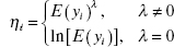
Considerable resources were deployed against the A-4 and A-6, including small arms, AAA or antiaircraft artillery, and surface-to-air missiles. Table 13.6 contains data from 30 strike missions involving these two types of aircraft. The regressor x1 is an indicator variable (A-4 = 0 and A-6 = 1), and the other regressors x2 and x3 are bomb load (in tons) and total months of aircrew experience. The response variable is the number of locations where damage was inflicted on the aircraft.
TABLE 13.6 Aircraft Damage Data

We will model the damage response as a function of the three regressors. Since the response is a count, we will use a Poisson regression model with the log link. Table 13.7 presents some of the output from SAS PROC GENMOD a widely used software package for fitting generalized linear models, which include Poisson regression. The SAS code for this example is
proc genmod;
model y = xl x2 x3 / dist = poisson type1 type3;
The Type 1 analysis is similar to the Type 1 sum of squares analysis, also known as the sequential sum of squares analysis. The test on any given term is conditional based on all previous terms in the analysis being included in the model. The intercept is always assumed in the model, which is why the Type 1 analysis begins with the term x1, which is the first term specified in the model statement. The Type 3 analysis is similar to the individual t-tests in that it is a test of the contribution of the specific term given all the other terms in the model. The model in the first page of the table uses all three regressors. The model adequacy checks based on deviance and the Pearson chi-square statistics are satisfactory, but we notice that x3 = crew experience is not significant, using both the Wald test and the type 3 partial deviance (notice that the Wald statistic reported is ![]() , which is referred to a chi-square distribution with a single degree of freedom). This is a reasonable indication that x3 can be removed from the model. When x3 is removed, however, it turns out that now x1 = type of aircraft is no longer significant (you can easily verify that the type 3 partial deviance for x1 in this model has a P value of 0.1582). A moment of reflection on the data in Table 13.6 will reveal that there is a lot of multicollinearity in the data. Essentially, the A-6 is a larger aircraft so it will carry a heavier bomb load, and because it has a two-man crew, it may tend to have more total months of crew experience. Therefore, as x1 increases, there is a tendency for both of the other regressors to also increase.
, which is referred to a chi-square distribution with a single degree of freedom). This is a reasonable indication that x3 can be removed from the model. When x3 is removed, however, it turns out that now x1 = type of aircraft is no longer significant (you can easily verify that the type 3 partial deviance for x1 in this model has a P value of 0.1582). A moment of reflection on the data in Table 13.6 will reveal that there is a lot of multicollinearity in the data. Essentially, the A-6 is a larger aircraft so it will carry a heavier bomb load, and because it has a two-man crew, it may tend to have more total months of crew experience. Therefore, as x1 increases, there is a tendency for both of the other regressors to also increase.
TABLE 13.7 SAS PROC GENMOD Output for Aircraft Damage Data in Example 13.8


To investigate the potential usefulness of various subset models, we fit all three two-variable models and all three one-variable models to the data in Table 13.6. A brief summary of the results obtained is as follows:
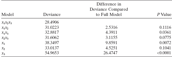
From examining the difference in deviance between each of the subset models and the full model, we notice that deleting either x1 or x2 results in a two-variable model that is significantly worse than the full model. Removing x3 results in a model that is not significantly different than the full model, but as we have already noted, x1 is not significant in this model. This leads us to consider the one-variable models. Only one of these models, the one containing x2, is not significantly different from the full model. The SAS PROC GENMOD output for this model is shown in the second page of Table 13.7. The Poisson regression model for predicting damage is
![]()
The deviance for this model is D(β) = 33.0137 with 28 degrees of freedom, and the P value is 0.2352, so we conclude that the model is an adequate fit to the data.
13.4 THE GENERALIZED LINEAR MODEL
All of the regression models that we have considered in the two previous sections of this chapter belong to a family of regression models called the generalized linear model (GLM). The GLM is actually a unifying approach to regression and experimental design models, uniting the usual normal-theory linear regression models and nonlinear models such as logistic and Poisson regression.
A key assumption in the GLM is that the response variable distribution is a member of the exponential family of distributions, which includes (among others) the normal, binomial, Poisson, inverse normal, exponential, and gamma distributions. Distributions that are members of the exponential family have the general form
where φ is a scale parameter and θi is called the natural location parameter. For members of the exponential family,
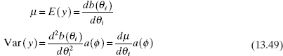
where Var(μ) denotes the dependence of the variance of the response on its mean. This is a characteristic of all distributions that are a member of the exponential family, except for the normal distribution. As a result of Eq. (13.50), we have
In Appendix C.14 we show that the normal, binomial, and Poisson distributions are members of the exponential family.
13.4.1 Link Functions and Linear Predictors
The basic idea of a GLM is to develop a linear model for an appropriate function of the expected value of the response variable. Let ηi be the linear predictor defined by
Note that the expected response is just
We call the function g the link function. Recall that we introduced the concept of a link function in our description of Poisson regression. There are many possible choices of the link function, but if we choose
we say that ηi is the canonical link. Table 13.8 shows the canonical links for the most common choices of distributions employed with the GLM.
TABLE 13.8 Canonical Links for the Generalized Linear Model
| Distribution | Canonical Link |
| Normal | η = μi (identity link) |
| Binomial | |
| Poisson | ηi = ln(λ) (log link) |
| Exponential | |
| Gamma |
There are other link functions that could be used with a GLM, including:
- The probit link,

where Φ represents the cumulative standard normal distribution function.
- The complementary log-log link,
- The power family link,
A very fundamental idea is that there are two components to a GLM: the response distribution and the link function. We can view the selection of the link function in a vein similar to the choice of a transformation on the response. However, unlike a transformation, the link function takes advantage of the natural distribution of the response. Just as not using an appropriate transformation can result in problems with a fitted linear model, improper choices of the link function can also result in significant problems with a GLM.
13.4.2 Parameter Estimation and Inference in the GLM
The method of maximum likelihood is the theoretical basis for parameter estimation in the GLM. However, the actual implementation of maximum likelihood results in an algorithm based on IRLS. This is exactly what we saw previously for the special cases of logistic and Poisson regression. We present the details of the procedure in Appendix C.14. In this chapter, we rely on SAS PROC GENMOD for model fitting and inference.
If ![]() is the final value of the regression coefficients that the IRLS algorithm produces and if the model assumptions, including the choice of the link function, are correct, then we can show that asymptotically
is the final value of the regression coefficients that the IRLS algorithm produces and if the model assumptions, including the choice of the link function, are correct, then we can show that asymptotically
where the matrix V is a diagonal matrix formed from the variances of the estimated parameters in the linear predictor, apart from a(φ).
Some important observations about the GLM are as follows:
- Typically, when experimenters and data analysts use a transformation, they use OLS to actually fit the model in the transformed scale.
- In a GLM, we recognize that the variance of the response is not constant, and we use weighted least squares as the basis of parameter estimation.
- This suggests that a GLM should outperform standard analyses using transformations when a problem remains with constant variance after taking the transformation.
- All of the inference we described previously on logistic regression carries over directly to the GLM. That is, model deviance can be used to test for overall model fit, and the difference in deviance between a full and a reduced model can be used to test hypotheses about subsets of parameters in the model. Wald inference can be applied to test hypotheses and construct confidence intervals about individual model parameters.
Example 13.9 The Worsted Yarn Experiment
Table 13.9 contains data from an experiment conducted to investigate the three factors x1 = length, x2 = amplitude, and x3 = load on the cycles to failure y of worsted yarn. The regressor variables are coded, and readers who have familiarity with designed experiments will recognize that the experimenters here used a 33 factorial design. The data also appear in Box and Draper [1987] and Myers, Montgomery, and Anderson-Cook [2009]. These authors use the data to illustrate the utility of variance-stabilizing transformations. Both Box and Draper [1987] and Myers, Montgomery, and Anderson-Cook [2009] show that the log transformation is very effective in stabilizing the variance of the cycles-to-failure response. The least-squares model is
TABLE 13.9 Data from the Worsted Yarn Experiment
![]()
The response variable in this experiment is an example of a nonnegative response that would be expected to have an asymmetric distribution with a long right tail. Failure data are frequently modeled with exponential, Weibull, lognormal, or gamma distributions both because they possess the anticipated shape and because sometimes there is theoretical or empirical justification for a particular distribution.
We will model the cycles-to-failure data with a GLM using the gamma distribution and the log link. From Table 13.8 we observe that the canonical link here is the inverse link; however, the log link is often a very effective choice with the gamma distribution.
Table 13.10 presents some summary output information from SAS PROC GENMOD for the worsted yarn data. The appropriate SAS code is
proc genmod;
model y = x1 x2 x3 / dist = gamma link = log typel type3;
Notice that the fitted model is
![]()
which is virtually identical to the model obtained via data transformation. Actually, since the log transformation works very well here, it is not too surprising that the GLM produces an almost identical model. Recall that we observed that the GLM is most likely to be an effective alternative to a data transformation when the transformation fails to produce the desired properties of constant variance and approximate normality in the response variable.
For the gamma response case, it is appropriate to use the scaled deviance in the SAS output as a measure of the overall fit of the model. This quantity would be compared to the chi-square distribution with n − p degrees of freedom, as usual. From Table 13.10 we find that the scaled deviance is 27.1276, and referring this to a chi-square distribution with 23 degrees of freedom gives a P value of approximately 0.25, so there is no indication of model inadequacy from the deviance criterion. Notice that the scaled deviance divided by its degrees of freedom is also close to unity. Table 13.10 also gives the Wald tests and the partial deviance statistics (both type 1 or “effects added in order” and type 3 or “effects added last” analyses) for each regressor in the model. These test statistics indicate that all three regressors are important predictors and should be included in the model.
13.4.3 Prediction and Estimation with the GLM
For any generalized linear model, the estimate of the mean response at some point of interest, say x0, is
TABLE 13.10 SAS PROC GENMOD Output for the Worsted Yarn Experiment

where g is the link function and it is understood that x0 may be expanded to model form if necessary to accommodate terms such as interactions that may have been included in the linear predictor. An approximate confidence interval on the mean response at this point can be computed as follows. Let Σ be the asymptotic variance–covariance matrix for ![]() ; thus,
; thus,
![]()
The asymptotic variance of the estimated linear predictor at x0 is
![]()
Thus, an estimate of this variance is ![]() , where
, where ![]() is the estimated variance–covariance matrix of
is the estimated variance–covariance matrix of ![]() . The 100(1 − α) percent confidence interval on the true mean response at the point x0 is
. The 100(1 − α) percent confidence interval on the true mean response at the point x0 is
where
This method is used to compute the confidence intervals on the mean response reported in SAS PROC GENMOD. This method for finding the confidence intervals usually works well in practice, because ![]() is a maximum-likelihood estimate, and therefore any function of
is a maximum-likelihood estimate, and therefore any function of ![]() is also a maximum-likelihood estimate. The above procedure simply constructs a confidence interval in the space defined by the linear predictor and then transforms that interval back to the original metric.
is also a maximum-likelihood estimate. The above procedure simply constructs a confidence interval in the space defined by the linear predictor and then transforms that interval back to the original metric.
It is also possible to use Wald inference to derive other expressions for approximate confidence intervals on the mean response. Refer to Myers, Montgomery, and Anderson-Cook [2009] for the details.
Example 13.10 The Worsted Yarn Experiment
Table 13.11 presents three sets of confidence intervals on the mean response for the worsted yarn experiment originally described in Example 13.10. In this table, we have shown 95% confidence intervals on the mean response for all 27 points in the original experimental data for three models: the least-squares model in the log scale, the untransformed response from this least-squares model, and the GLM (gamma response distribution and log link). The GLM confidence intervals were computed from Eq. (13.58). The last two columns of Table 13.11 compare the lengths of the normal-theory least-squares confidence intervals from the untransformed response to those from the GLM. Notice that the lengths of the GLM intervals are uniformly shorter that those from the least-squares analysis based on transformations. So even though the prediction equations produced by these two techniques are very similar (as we noted in Example 13.9), there is some evidence to indicate that the predictions obtained from the GLM are more precise in the sense that the confidence intervals will be shorter.
13.4.4 Residual Analysis in the GLM
Just as in any model-fitting procedure, analysis of residuals is important in fitting the GLM. Residuals can provide guidance concerning the overall adequacy of the model, assist in verifying assumptions, and give an indication concerning the appropriateness of the selected link function.
TABLE 13.11 Comparison of 95% Confidence Intervals on the Mean Response for the Worsted Yarn Data

The ordinary or raw residuals from the GLM are just the differences between the observations and the fitted values,
It is generally recommended that residual analysis in the GLM be performed using deviance residuals. Recall that the ith deviance residual is defined as the square root of the contribution of the ith observation to the deviance multiplied by the sign of the ordinary residual. Equation (13.30) gave the deviance residual for logistic regression. For Poisson regression with a log link, the deviance residuals are
![]()
where the sign is the sign of the ordinary residual. Notice that as the observed value of the response yi and the predicted value ![]() become closer to each other, the deviance residuals approach zero.
become closer to each other, the deviance residuals approach zero.
Generally, deviance residuals behave much like ordinary residuals do in a standard normal-theory linear regression model. Thus, plotting the deviance residuals on a normal probability scale and versus fitted values is a logical diagnostic. When plotting deviance residuals versus fitted values, it is customary to transform the fitted values to a constant information scale. Thus,
- For normal responses, use
 .
. - For binomial responses, use
 .
. - For Poisson responses, use
 .
. - For gamma responses, use
 .
.
Example 13.11 The Worsted Yarn Experiment
Table 13.12 presents the actual observations from the worsted yarn experiment in Example 13.9, along with the predicted values from the GLM (gamma response with log link) that was fit to the data, the raw residuals, and the deviance residuals. These quantities were computed using SAS PROC GENMOD. Figure 13.7a is a normal probability plot of the deviance residuals and Figure 13.7b is a plot of the deviance residuals versus the “constant information” fitted values, ![]() . The normal probability plot of the deviance residuals is generally satisfactory, while the plot of the deviance residuals versus the fitted values indicates that one of the observations may be a very mild outlier. Neither plot gives any significant indication of model inadequacy, however, so we conclude that the GLM with gamma response variable distribution and a log link is a very satisfactory model for the cycles-to-failure response.
. The normal probability plot of the deviance residuals is generally satisfactory, while the plot of the deviance residuals versus the fitted values indicates that one of the observations may be a very mild outlier. Neither plot gives any significant indication of model inadequacy, however, so we conclude that the GLM with gamma response variable distribution and a log link is a very satisfactory model for the cycles-to-failure response.
13.4.5 Using R to Perform GLM Analysis
The workhorse routine within R for analyzing a GLM is “glm.” The basic form of this statement is:
TABLE 13.12 Predicted Values and Residuals from the Worsted Yarn Experiment


Figure 13.7 Plots of the deviance residuals from the GLM for the worsted yarn data. (a) Normal probability plot of deviance results. (b) Plot of the deviance residuals versus ![]()
The formula specification is exactly the same as for a standard linear model. For example, the formaula for the model η = β0 + β1x1 + β2x2 is
y ~ x1+x2
The choices for family and the links available are:
- binomial (logit, probit, log, complementary loglog),
- gaussian (identity, log, inverse),
- Gamma (identity, inverse, log)
- inverse.gaussian (1/μ2, identity, inverse, log)
- poisson (identity, log, square root), and
- quasi (logit, probit, complementary loglog, identity, inverse, log, 1/μ2, square root).
R is case-sensitive, so the family is Gamma, not gamma. By default, R uses the canonical link. To specify the probit link for the binomial family, the appropriate family phrase is binomial (link = probit).
R can produce two different predicted values. The “fit” is the vector of predicted values on the original scale. The “linear.predictor” is the vector of the predicted values for the linear predictor. R can produce the raw, the Pearson, and the deviance residuals. R also can produce the “influence measures,” which are the individual observation deleted statistics. The easiest way to put all this together is through examples.
We first consider the pneumoconiosis data from Example 13.1. The data set is small, so we do not need a separate data file. The R code is:
> years <- c(5.8, 15.0, 21.5, 27.5, 33.5, 39.5, 46.0, 51.5)
> cases <- c(0, 1, 3, 8, 9, 8, 10, 5)
> miners <- c(98, 54, 43, 48, 51, 38, 28, 11)
> ymat <- cbind(cases, miners-cases)
> ashford <- data.frame(ymat, years)
> anal <- glm(ymat ? years, family=binomial, data=ashford)
summary(anal)
pred_prob <- anal$fit
eta_hat <- anal$linear.predictor
dev_res <- residuals(anal, c=”deviance”)
influence.measures(anal)
df <- dfbetas(anal)
df_int <- df[,1]
df_years <- df[,2]
hat <- hatvalues(anal)
qqnorm(dev_res)
plot(pred_prob,dev_res)
plot(eta_hat,dev_res)
plot(years,dev_res)
plot(hat,dev_res)
plot(pred_prob,df_years)
plot(hat,df_years)
ashford2 <- cbind(ashford,pred_prob,eta_hat,dev_res,df_int,
df_years,hat)
write.table(ashford2, ?ashford_output.txt?)
We next consider the Aircraft Damage example from Example 13.8. The data are in the file aircraft_damage_data.txt. The appropriate R code is
air <- read.table(?aircraft_damage_data.txt?,header=TRUE, sep=??)
air.model <- glm(y?x1+x2+x3, dist=?poisson?, data=air)
summary(air.model)
print(influence.measures(air.model))
yhat <- air.model$fit
dev_res <- residuals(air.model, c=?deviance?)
qqnorm(dev_res)
plot(yhat,dev_res)
plot(air$x1,dev_res)
plot(air$x2,dev_res)
plot(air$x3,dev_res)
air2 <- cbind(air,yhat,dev_res)
write.table(air2, ?aircraft damage_output.txt?)
Finally, consider the Worsted Yarn example from Example 13.9. The data are in the file worsted_data.txt. The appropriate R code is
yarn <- read.table(?worsted_data.txt?,header=TRUE, sep=??)
yarn.model <- glm(y?x1+x2+x3, dist=Gamma(link=log), data=air)
summary(yarn.model)
print(influence.measures(yarn.model))
yhat <- air.model$fit
dev_res <- residuals(yarn.model, c=?deviance?)
qqnorm(dev_res)
plot(yhat,dev_res)
plot(yarn$x1,dev_res)
plot(yarn$x2,dev_res)
plot(yarn$x3,dev_res)
yarn2 <- cbind(yarn,yhat,dev_res)
write.table(yarn2, ?yarn_output.txt?)
13.4.6 Overdispersion
Overdispersion is a phenomenon that sometimes occurs when we are modeling response data with either a binomial or Poisson distribution. Basically, it means that the variance of the response is greater than one would anticipate for that choice of response distribution. An overdispersion condition is often diagnosed by evaluating the value of model deviance divided by degrees of freedom. If this value greatly exceeds unity, then overdispersion is a possible source of concern.
The most direct way to model this situation is to allow the variance function of the binomial or Poisson distributions to have a multiplicative dispersion factor φ, so that

The models are fit in the usual manner, and the values of the model parameters are not affected by the value of φ. The parameter φ can be specified directly if its value is known or it can be estimated if there is replication of some data points. Alternatively, it can be directly estimated. A logical estimate for φ is the deviance divided by its degrees of freedom. The covariance matrix of model coefficients is multiplied by φ and the scaled deviance and log-likelihoods used in hypothesis testing are divided by φ.
The function obtained by dividing a log-likelihood by φ for the binomial or Poisson error distribution case is no longer a proper log-likelihood function. It is an example of a quasi-likelihood function. Fortunately, most of the asymptotic theory for log-likelihoods applies to quasi-likelihoods, so we can justify computing approximate standard errors and deviance statistics just as we have done previously.
PROBLEMS
13.1 The table below presents the test-firing results for 25 surface-to-air antiaircraft missiles at targets of varying speed. The result of each test is either a hit (y = 1) or a miss (y = 0).
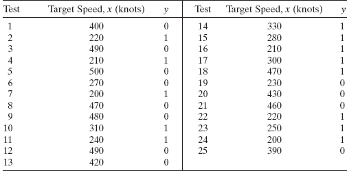
- Fit a logistic regression model to the response variable y. Use a simple linear regression model as the structure for the linear predictor.
- Does the model deviance indicate that the logistic regression model from part a is adequate?
- Provide an interpretation of the parameter β1 in this model.
- Expand the linear predictor to include a quadratic term in target speed. Is there any evidence that this quadratic term is required in the model?
13.2 A study was conducted attempting to relate home ownership to family income. Twenty households were selected and family income was estimated, along with information concerning home ownership (y = 1 indicates yes and y = 0 indicates no). The data are shown below.

- Fit a logistic regression model to the response variable y. Use a simple linear regression model as the structure for the linear predictor.
- Does the model deviance indicate that the logistic regression model from part a is adequate?
- Provide an interpretation of the parameter β1 in this model.
- Expand the linear predictor to include a quadratic term in income. Is there any evidence that this quadratic term is required in the model?
13.3 The compressive strength of an alloy fastener used in aircraft construction is being studied. Ten loads were selected over the range 2500–4300 psi and a number of fasteners were tested at those loads. The numbers of fasteners failing at each load were recorded. The complete test data are shown below.
| Load, x (psi) | Sample Size, n | Number Failing, r |
| 2500 | 50 | 10 |
| 2700 | 70 | 17 |
| 2900 | 100 | 30 |
| 3100 | 60 | 21 |
| 3300 | 40 | 18 |
| 3500 | 85 | 43 |
| 3700 | 90 | 54 |
| 3900 | 50 | 33 |
| 4100 | 80 | 60 |
| 4300 | 65 | 51 |
- Fit a logistic regression model to the data. Use a simple linear regression model as the structure for the linear predictor.
- Does the model deviance indicate that the logistic regression model from part a is adequate?
- Expand the linear predictor to include a quadratic term. Is there any evidence that this quadratic term is required in the model?
- For the quadratic model in part c, find Wald statistics for each individual model parameter.
- Find approximate 95% confidence intervals on the model parameters for the quadratic model from part c.
13.4 The market research department of a soft drink manufacturer is investigating the effectiveness of a price discount coupon on the purchase of a two-liter beverage product. A sample of 5500 customers was given coupons for varying price discounts between 5 and 25 cents. The response variable was the number of coupons in each price discount category redeemed after one month. The data are shown below.
| Discount, x | Sample Size, n | Number Redeemed, r |
| 5 | 500 | 100 |
| 7 | 500 | 122 |
| 9 | 500 | 147 |
| 11 | 500 | 176 |
| 13 | 500 | 211 |
| 15 | 500 | 244 |
| 17 | 500 | 277 |
| 19 | 500 | 310 |
| 21 | 500 | 343 |
| 23 | 500 | 372 |
| 25 | 500 | 391 |
- Fit a logistic regression model to the data. Use a simple linear regression model as the structure for the linear predictor.
- Does the model deviance indicate that the logistic regression model from part a is adequate?
- Draw a graph of the data and the fitted logistic regression model.
- Expand the linear predictor to include a quadratic term. Is there any evidence that this quadratic term is required in the model?
- Draw a graph of this new model on the same plot that you prepared in part c. Does the expanded model visually provide a better fit to the data than the original model from part a?
- For the quadratic model in part d, find Wald statistics for each individual model parameter.
- Find approximate 95% confidence intervals on the model parameters for the quadratic logistic regression model from part d.
13.5 A study was performed to investigate new automobile purchases. A sample of 20 families was selected. Each family was surveyed to determine the age of their oldest vehicle and their total family income. A follow-up survey was conducted 6 months later to determine if they had actually purchased a new vehicle during that time period (y = 1 indicates yes and y = 0 indicates no). The data from this study are shown in the following table.

- Fit a logistic regression model to the data.
- Does the model deviance indicate that the logistic regression model from part a is adequate?
- Interpret the model coefficients β1 and β2.
- What is the estimated probability that a family with an income of $45,000 and a car that is 5 years old will purchase a new vehicle in the next 6 months?
- Expand the linear predictor to include an interaction term. Is there any evidence that this term is required in the model?
- For the model in part a, find statistics for each individual model parameter.
- Find approximate 95% confidence intervals on the model parameters for the logistic regression model from part a.
13.6 A chemical manufacturer has maintained records on the number of failures of a particular type of valve used in its processing unit and the length of time (months) since the valve was installed. The data are shown below.

- Fit a Poisson regression model to the data.
- Does the model deviance indicate that the Poisson regression model from part a is adequate?
- Construct a graph of the fitted model versus months. Also plot the observed number of failures on this graph.
- Expand the linear predictor to include a quadratic term. Is there any evidence that this term is required in the model?
- For the model in part a, find Wald statistics for each individual model parameter.
- Find approximate 95% confidence intervals on the model parameters for the Poisson regression model from part a.
13.7 Myers [1990] presents data on the number of fractures (y) that occur in the upper seams of coal mines in the Appalachian region of western Virginia. Four regressors were reported: x1 = inner burden thickness (feet), the shortest distance between seam floor and the lower seam; x2 = percent extraction of the lower previously mined seam; x3 = lower seam height (feet); and x4 = time (years) that the mine has been in operation. The data are shown below.

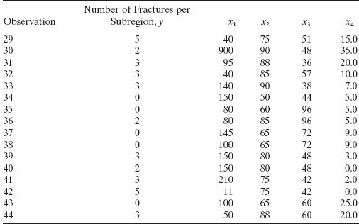
- Fit a Poisson regression model to these data using the log link.
- Does the model deviance indicate that the model from part a is satisfactory?
- Perform a type 3 partial deviance analysis of the model parameters. Does this indicate that any regressors could be removed from the model?
- Compute Wald statistics for testing the contribution of each regressor to the model. Interpret the results of these test statistics.
- Find approximate 95% Wald confidence intervals on the model parameters.
13.8 Reconsider the mine fracture data from Problem 13.7. Remove any regressors from the original model that you think might be unimportant and rework parts b–e of Problem 13.7. Comment on your findings.
13.9 Reconsider the mine fracture data from Problems 13.7 and 13.8. Construct plots of the deviance residuals from the best model you found and comment on the plots. Does the model appear satisfactory from a residual analysis viewpoint?
13.10?Reconsider the model for the automobile purchase data from Problem 13.5, part a. Construct plots of the deviance residuals from the model and comment on these plots. Does the model appear satisfactory from a residual analysis viewpoint?
13.11 Reconsider the model for the soft drink coupon data from Problem 13.4, part a. Construct plots of the deviance residuals from the model and comment on these plots. Does the model appear satisfactory from a residual analysis viewpoint?
13.12 Reconsider the model for the aircraft fastener data from Problem 13.3, part a. Construct plots of the deviance residuals from the model and comment on these plots. Does the model appear satisfactory from a residual analysis viewpoint?
13.13 The gamma probability density function is
![]()
Show that the gamma is a member of the exponential family.
13.14 The exponential probability density function is
![]()
Show that the exponential distribution is a member of the exponential family.
13.15 The negative binomial probability mass function is
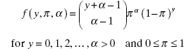
Show that the negative binomial is a member of the exponential family.
13.16 The data in the table below are from an experiment designed to study the advance rate y of a drill. The four design factors are x1 = load, x2 = flow, x3 = drilling speed, and x4 = type of drilling mud (the original experiment is described by Cuthbert Daniel in his 1976 book on industrial experimentation).

- Fit a generalized linear model to the advance rate response. Use a gamma response distribution and a log link, and include all four regressors in the linear predictor.
- Find the model deviance for the GLM from part a. Does this indicate that the model is satisfactory?
- Perform a type 3 partial deviance analysis of the model parameters. Does this indicate that any regressors could be removed from the model?
- Compute Wald statistics for testing the contribution of each regressor to the model. Interpret the results of these test statistics.
- Find approximate 95% Wald confidence intervals on the model parameters.
13.17 Reconsider the drill data from Problem 13.16. Remove any regressors from the original model that you think might be unimportant and rework parts b–e of Problem 13.16. Comment on your findings.
13.18 Reconsider the drill data from Problem 13.16. Fit a GLM using the log link and the gamma distribution, but expand the linear predictor to include all six of the two-factor interactions involving the four original regressors. Compare the model deviance for this model to the model deviance for the “main effects only model” from Problem 13.16. Does adding the interaction terms seem useful?
13.19 Reconsider the model for the drill data from Problem 13.16. Construct plots of the deviance residuals from the model and comment on these plots. Does the model appear satisfactory from a residual analysis viewpoint?
13.20 The table below shows the predicted values and deviance residuals for the Poisson regression model using x2 = bomb load as the regressor fit to the aircraft damage data in Example 13.8. Plot the residuals and comment on model adequacy.


13.21 Consider a logistic regression model with a linear predictor that includes an interaction term, say x′β = β0 + β1x1 + β2x2 + β12x1x2. Derive an expression for the odds ratio for the regressor x1. Does this have the same interpretation as in the case where the linear predictor does not have the interaction term?
13.22 The theory of maximum-likelihood states that the estimated large-sample covariance for maximum-likelihood estimates is the inverse of the information matrix, where the elements of the information matrix are the negatives of the expected values of the second partial derivatives of the log-likelihood function evaluated at the maximum-likelihood estimates. Consider the linear regression model with normal errors. Find the information matrix and the covariance matrix of the maximum-likelihood estimates.
13.23 Consider the automobile purchase late in Problem 13.5. Fit models using both the probit and complementary log-log functions. Compare three models to the one obtained using the logit.
13.24 Reconsider the pneumoconiosis data in Table 13.1. Fit models using both the probit and complimentary log-log functions. Compare these models to the one obtained in Example 13.1 using the logit.
13.25 On 28 January 1986 the space shuttle Challenger was destroyed in an explosion shortly after launch from Cape Kennedy. The cause of the explosion was eventually identified as catastrophic failure of the O-rings on the solid rocket booster. The failure likely occurred because the O-ring material was subjected to a lower temperature at launch (31°F) than was appropriate. The material and the solid rocket joints had never been tested at temperatures this low. Some O-ring failures had occurred during other shuttle launches (or engine static tests). The failure data observed prior to the Challenger launch is shown in the following table.

- Fit a logistic regression model to these data. Construct a graph of the data and display the fitted model. Discuss how well the model fits the data.
- Calculate and interpret the odds ratio.
- What is the estimated failure probability at 50°F?
- What is the estimated failure probability at 75°F?
- What is the estimated failure probability at 31°F? Notice that there is extrapolation involved in obtaining this estimate. What influence would that have on your recommendation about launching the space shuttle?
- Calculate and analyze the deviance residuals for this model.
- Add a quadratic term in temperature to the logistic regression model in part a. Is there any evidence that this term improves the model?
13.26 A student conducted a project looking at the impact of popping temperature, amount of oil, and the popping time on the number of inedible kernels of popcorn. The data follow. Analyze these data using Poisson regression.
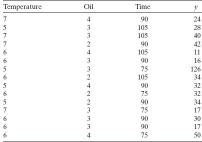
13.27 Bailer and Piegorsch [2000] report on an experiment that examines the effect of a herbicide, nitrofen, on the umber of offspring produced by a particular freshwater invertebrate zooplankton. The data follow. Perform an appropriate analysis of these data.
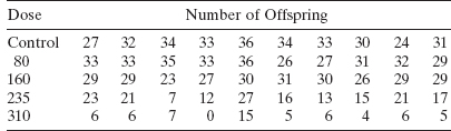
13.28 Chapman [1997–98] conducted an experiment using accelerated life testing to determine the estimated shelf life of a photographic developer. The data follow. Lifetimes often follow an exponential distribution. This company has found that the maximum density is a good indicator of overall developer/film performance; correspondingly using generalized linear models. Perform appropriate residual analysis of your final model.
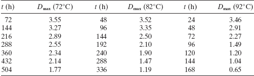
13.29 Gupta and Das [2000] performed an experiment to improve the resistivity of a urea formaldehyde resin. The factors were amount of sodium hydroxide, A, reflux time, B, solvent distillate, C, phthalic anhydride, D, water collection time, E, and solvent distillate collection time, F. The data follow, where y1 is the resistivity from the first replicate of the experiment and y2 is the resistivity from the second replicate. Assume a gamma distribution. Use both the canonical and the log link to analyze these data. Perform appropriate residual analysis of your final models.

