CHAPTER 11

VALIDATION OF REGRESSION MODELS

11.1 INTRODUCTION

Regression models are used extensively for prediction or estimation, data description, parameter estimation, and control. Frequently the user of the regression model is a different individual from the model developer. Before the model is released to the user, some assessment of its validity should be made. We distinguish between model adequacy checking and model validation. Model adequacy checking includes residual analysis, testing for lack of fit, searching for high-leverage or overly influential observations, and other internal analyses that investigate the fit of the regression model to the available data. Model validation, however, is directed toward determining if the model will function successfully in its intended operating environment.

Since the fit of the model to the available data forms the basis for many of the techniques used in the model development process (such as variable selection), it is tempting to conclude that a model that fits the data well will also be successful in the final application. This is not necessarily so. For example, a model may have been developed primarily for predicting new observations. There is no assurance that the equation that provides the best fit to existing data will be a successful predictor. Influential factors that were unknown during the model-building stage may significantly affect the new observations, rendering the predictions almost useless. Furthermore, the correlative structure between the regressors may differ in the model-building and prediction data. This may result in poor predictive performance for the model. Proper validation of a model developed to predict new observations should involve testing the model in that environment before it is released to the user.

Another critical reason for validation is that the model developer often has little or no control over the model's final use. For example, a model may have been developed as an interpolation equation, but when the user discovers that it is successful in that respect, he or she will also extrapolate with it if the need arises, despite any warnings or cautions from the developer. Furthermore, if this extrapolation performs poorly, it is almost always the model developer and not the model user who is blamed for the failure. Regression model users will also frequently draw conclusions about the process being studied from the signs and magnitudes of the coefficients in their model, even though they have been cautioned about the hazards of interpreting partial regression coefficients. Model validation provides a measure of protection for both model developer and user.

Proper validation of a regression model should include a study of the coefficients to determine if their signs and magnitudes are reasonable. That is, can be reasonably interpreted as an estimate of the effect of x_j? We should also investigate the stability of the regression coefficients. That is, are the obtained from a new sample likely to be similar to the current coefficients? Finally, validation requires that the model's prediction performance be investigated. Both interpolation and extrapolation modes should be considered.

This chapter will discuss and illustrate several techniques useful in validating regression models. Several references on the general subject of validation are Brown, Durbin, and Evans [1975], Geisser [1975], McCarthy [1976], Snee [1977], and Stone [1974]. Snee's paper is particularly recommended.

11.2 VALIDATION TECHNIQUES

Three types of procedures are useful for validating a regression model:

1. Analysis of the model coefficients and predicted values including comparisons with prior experience, physical theory, and other analytical models or simulation results
2. Collection of new (or fresh) data with which to investigate the model's predictive performance
3. Data splitting, that is, setting aside some of the original data and using these observations to investigate the model's predictive performance

The final intended use of the model often indicates the appropriate validation methodology. Thus, validation of a model intended for use as a predictive equation should concentrate on determining the model's prediction accuracy. However, because the developer often does not control the use of the model, we recommend that, whenever possible, all the validation techniques above be used. We will now discuss and illustrate these techniques. For some additional examples, see Snee [1977].

11.2.1 Analysis of Model Coefficients and Predicted Values

The coefficients in the final regression model should be studied to determine if they are stable and if their signs and magnitudes are reasonable. Previous experience, theoretical considerations, or an analytical model can often provide information concerning the direction and relative size of the effects of the regressors. The coefficients in the estimated model should be compared with this information. Coefficients with unexpected signs or that are too large in absolute value often indicate either an inappropriate model (missing or misspecified regressors) or poor estimates of the effects of the individual regressors. The variance inflation factors and the other multicollinearity diagnostics in Chapter 19 also are an important guide to the validity of the model. If any VIF exceeds 5 or 10, that particular coefficient is poorly estimated or unstable because of near-linear dependences among the regressors. When the data are collected across time, we can examine the stability of the coefficients by fitting the model on shorter time spans. For example, if we had several years of monthly data, we could build a model for each year. Hopefully, the coefficients for each year would be similar.

The predicted response values can also provide a measure of model validity. Unrealistic predicted values such as negative predictions of a positive quantity or predictions that fall outside the anticipated range of the response, indicate poorly estimated coefficients or an incorrect model form. Predicted values inside and on the boundary of the regressor variable bull provide a measure of the model's interpolation performance. Predicted values outside this region are a measure of extrapolation performance.

Example 11.1 The Bald Cement Data

Consider the Hald cement data introduced in Example 10.1. We used all possible regressions to develop two possible models for these data, model 1,

and model 2,

Note that the regression coefficient for x₁ is very similar in both models, although the intercepts are very different and the coefficients of x₂ are moderately different. In Table 10.5 we calculated the values of the PRESS statistic, R²_Prediction, and the VIFs for both models. For model 1 both VIFs are very small, indicating no potential problems with multicollinearity. However, for model 2, the VIFs associated with x₂ and x₄ exceed 10, indicating that moderate problems with multicollinearity are present. Because multicollinearity often impacts the predictive performance of a regression model, a reasonable initial validation effort would be to examine the predicted values to see if anything unusual is apparent. Table 11.1 presents the predicted values corresponding to each individual observation for both models. The predicted values are virtually identical for both models, so there is little reason to believe that either model is inappropriate based on this test of prediction performance. However, this is only a relative simple test of model prediction performance, not a study of how either model would perform if moderate extrapolation were required. Based in this simple analysis of coefficients and predicted values, there is little reason to doubt the validity of either model, but as noted in Example 10.1, we would probably prefer model 1 because it has fewer parameters and smaller VIFs.

TABLE 11.1 Prediction Values for Two Models for Hald Cement Data

11.2.2 Collecting Fresh Data—Confirmation Runs

The most effective method of validating a regression model with respect to its prediction performance is to collect new data and directly compare the model predictions against them. If the model gives accurate predictions of new data, the user will have greater confidence in both the model and the model-building process. Sometimes these new observations are called confirmation runs. At least 15–20 new observations are desirable to give a reliable assessment of the model's prediction performance. In situations where two or more alternative regression models have been developed from the data, comparing the prediction performance of these models on new data may provide a basis for final model selection.

Example 11.2 The Delivery Time Data

Consider the delivery time data introduced in Example 3.1. We have previously developed a least-squares fit for these data. The objective of fitting the regression model is to predict new observations. We will investigate the validity of the least-squares model by predicting the delivery time for fresh data.

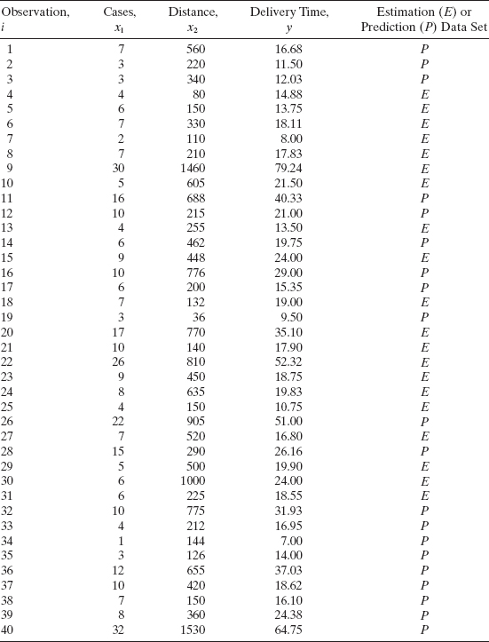
Recall that the original 25 observations came from four cities: Austin, San Diego, Boston, and Minneapolis. Fifteen new observations from Austin, Boston, San Diego, and a fifth city, Louisville, are shown in Table 11.2, along with the corresponding predicted delivery times and prediction errors from the least-squares fit ŷ = 2.3412 + 1.6159x₁ + 0.0144x₂ (columns 5 and 6). Note that this prediction data set consists of 11 observations from cities used in the original data collection process and 4 observations from a new city. This mix of old and new cities may provide some information on how well the two models predict at sites where the original data were collected and at new sites.

Column 6 of Table 11.2 shows the prediction errors for the least-squares model. The average prediction error is 0.4060, which is nearly zero, so that model seems to produce approximately unbiased predictions. There is only one relatively large prediction error, associated with the last observation from Louisville. Checking the original data reveals that this observation is an extrapolation point. Furthermore, this point is quite similar to point 9, which we know to be influential. From an overall perspective, these prediction errors increase our confidence in the usefulness of the model. Note that the prediction errors are generally larger than the residuals from the least-squares fit. This is easily seen by comparing the residual mean square

TABLE 11.2 Prediction Data Set for the Delivery Time Example

from the fitted model and the average squared prediction error

from the new prediction data. Since MS_Res (which may be thought of as the average variance of the residuals from the fit) is smaller than the average squared prediction error, the least-squares regression model does not predict new data as well as it fits the existing data. However, the degradation of performance is not severe, and so we conclude that the least-squares model is likely to be successful as a predictor. Note also that apart from the one extrapolation point the prediction errors from Louisville are not remarkably different from those experienced in the cities where the original data were collected. While the sample is small, this is an indication that the model may be portable. More extensive data collection at other sites would be helpful in verifying this conclusion.

It is also instructive to compare R² from the least-squares fit (0.9596) to the percentage of variability in the new data explained by the model, say

Once again, we see that the least-squares model does not predict new observations as well as it fits the original data. However, the “loss” in R² for prediction is slight.

Collecting new data has indicated that the least-squares fit for the delivery time data results in a reasonably good prediction equation. The interpolation parlormance of the model is likely to be better than when the model is used for extrapolation.

11.2.3 Data Splitting

In many situations, collecting new data for validation purposes is not possible. The data collection budget may already have been spent, the plant may have been converted to the production of other products or other equipment and resources needed for data collection may be unavailable. When these situations occur, a reasonable procedure is to split the available data into two parts, which Snee [1977] calls the estimation data and the prediction data. The estimation data are used to build the regression model, and the prediction data are then used to study the predictive ability of the model. Sometimes data splitting is called cross validation (see Mosteller and Tukey [1968] and Stone [1974]).

Data splitting may be done in several ways. For example, the PRESS statistic

is a form of data splitting. Recall that PRESS can be used in computing the R²-like statistic

that measures in an approximate sense how much of the variability in new observations the model might be expected to explain. To illustrate, recall that in Chapter 4 (Example 4.6) we calculated PRESS for the model fit to the original 25 observations on delivery time and found that PRESS = 457.4000. Therefore,

Now for the least-squares fit R² = 0.9596, so PRESS would indicate that the model is likely to be a very good predictor of new observations. Note that the R² for prediction based on PRESS is very similar to the actual prediction performance observed for this model with new data in Example 11.2.

If the data are collected in a time sequence, then time may be used as the basis of data splitting. That is, a particular time period is identified, and all observations collected before this time period are used to form the estimation data set, while observations collected later than this time period form the prediction data set. Fitting the model to the estimation data and examining its prediction accuracy for the prediction data would be a reasonable validation procedure to determine how the model is likely to perform in the future. This type of validation procedure is relatively common practice in time series analysis for investigating the potential performance of a forecasting model (for some examples, see Montgomery, Johnson, and Gardiner [1990]). For examples involving regression models, see Cady and Allen [1972] and Draper and Smith [1998].

In addition to time, other characteristics of the data can often be used for data splitting. For example, consider the delivery time data from Example 3.1 and assume that we had the additional 15 observations in Table 11.2 also available. Since there are five cities represented in the sample, we could use the observations from San Diego, Boston, and Minneapolis (for example) as the estimation data and the observations from Austin and Louisville as the prediction data. This would give 29 observations for estimation and 11 observations for validation. In other problem situations, we may find that operators, batches of raw materials, units of test equipment, laboratories, and so forth, can be used to form the estimation and prediction data sets. In cases where no logical basis of data splitting exists, one could randomly assign observations to the estimation and prediction data sets. If random allocations are used, one could repeat the process several times so that different subsets of observations are used for model fitting.

A potential disadvantage to these somewhat arbitrary methods of data splitting is that there is often no assurance that the prediction data set “stresses” the model severely enough. For example, a random division of the data would not necessarily ensure that some of the points in the prediction data set are extrapolation points, and the validation effort would provide no information on how well the model is likely to extrapolate. Using several different randomly selected estimation—prediction data sets would help solve this potential problem. In the absence of an obvious basis for data splitting, in some situations it might be helpful to have a formal procedure for choosing the estimation and prediction data sets.

Snee [1977] describes the DUPLEX algorithm for data splitting. He credits the development of the procedure to R. W. Kennard and notes that it is similar to the CADEX algorithm that Kennard and Stone [1969) proposed for design construction. The procedure utilizes the distance between all pairs of observations in the data set. The algorithm begins with a list of the n observations where the k regressors are standardized to unit length, that is,

where S_jj = Σⁿ_i=1(x_ij − _j)² is the corrected sum of squares of the jth regressor. The standardized regressors are then orthonormalized. This can be done by factoring the Z′Z matrix as

where T is a unique k × k upper triangular matrix. The elements of T can be found using the square root or Cholesky method (see Graybill [1976, pp. 231–236]). Then make the transformation

resulting in a new set of variables (the w's) that are orthogonal and have unit variance. This transformation makes the factor space more spherical.

Using the orthonormalized points, the Euclidean distance between all pairs of points is calculated. The pair of points that are the farthest apart is assigned to the estimation data set. This pair of points is removed from the list of points and the pair of remaining points that are the farthest apart is assigned to the prediction data set. Then this pair of points is removed from the list and the remaining point that is farthest from the pair of points in the estimation data set is included in the estimation data set. At the next step, the remaining unassigned point that is farthest from the two points in the prediction data set is added to the prediction data. The algorithm then continues to alternatively place the remaining points in either the estimation or prediction data sets until all n observations have been assigned.

Snee [1977] suggests measuring the statistical properties of the estimation and prediction data sets by comparing the pth root of the determinants of the X′X matrices for these two data sets, where p is the number of parameters in the model. The determinant of X′X is related to the volume of the region covered by the points. Thus, if X_E and X_P denote the X matrices for points in the estimation and prediction data sets, respectively, then

is a measure of the relative volumes of the regions spanned by the two data sets. Ideally this ratio should be close to unity. It may also be useful to examine the variance inflation factors for the two data sets and the eigenvalue spectra of X′_EX_E and X′_PX_P to measure the relative correlation between the regressors.

In using any data-splitting procedure (including the DUPLEX algorithm), several points should be kept in mind:

1. Some data sets may be too small to effectively use data splitting. Snee [1977] suggests that at least n ≥ 2p + 25 observations are required if the estimation and prediction data sets are of equal size, where p is the largest number of parameters likely to be required in the model. This sample size requirement ensures that there are a reasonable number of error degrees of freedom for the model.
2. Although the estimation and prediction data sets are often of equal size, one can split the data in any desired ratio. Typically the estimation data set would be larger than the prediction data set. Such splits are found by using the data-splitting procedure until the prediction data set contains the required number of points and then placing the remaining unassigned points in the estimation data set. Remember that the prediction data set should contain at least 15 points in order to obtain a reasonable assessment of model performance.
3. Replicates or points that are near neighbors in x space should be eliminated before splitting the data. Unless these replicates are eliminated, the estimation and prediction data sets may be very similar, and this would not necessarily test the model severely enough. In an extreme case where every point is replicated twice, the DUPLEX algorithm would form the estimation data set with one replicate and the prediction data set with the other replicate. The near-neighbor algorithm described in Section 4.5.2 may also be helpful. Once a set of near neighbors is identified, the average of the x coordinates of these points should be used in the data-splitting procedure.
4. A potential disadvantage of data splitting is that it reduces the precision with which regression coefficients are estimated. That is, the standard errors of the regression coefficients obtained from the estimation data set will be larger than they would have been if all the data had been used to estimate the coefficients. In large data sets, the standard errors may be small enough that this loss in precision is unimportant. However, the percentage increase in the standard errors can be large. If the model developed from the estimation data set is a satisfactory, predictor, one way to improve the precision of estimation is to reestimate the coefficients using the entire data set. The estimates of the coefficients in the two analyses should be very similar if the model is an adequate predictor of the prediction data set.
5. Double-cross validation may be useful in some problems. This is a procedure in which the data are first split into estimation and prediction data sets, a model developed from the estimation data, and its performance investigated using the prediction data. Then the roles of the two data sets are reversed; a model is developed using the original prediction data, and it is used to predict the original estimation data. The advantage of this procedure is that it provides two evaluations of model performance. The disadvantage is that there are now three models to choose from, the two developed via data splitting and the model fitted to all the data. If the model is a good predictor, it will make little difference which one is used, except that the standard errors of the coefficients in the model fitted to the total data set will be smaller. If there are major differences in predictive performance, coefficient estimates, or functional form for these models, then further analysis is necessary to discover the reasons for these differences.

Example 11.3 The Delivery Time Data

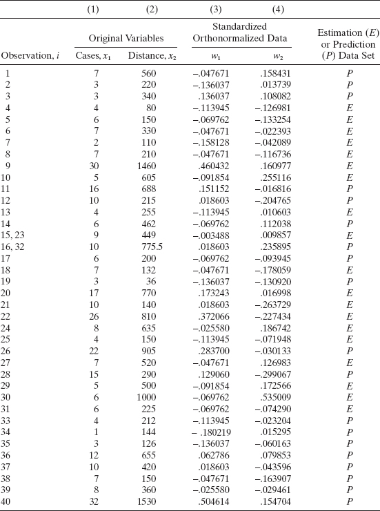
All 40 observations for the delivery time data in Examples 3.1 and 11.2 are shown in Table 11.3. We will assume that these 40 points were collected at one time and use the data set to illustrate data splitting with the DUPLEX algorithm. Since the model will have two regressors, an equal split of the data will give 17 error degrees of freedom for the estimation data. This is adequate, so DUPLEX can be used to generate the estimation and prediction data sets. An x₁ − x₂ plot is shown in Figure 11.1. Examination of the data reveals that there are two pairs of points that are near neighbors in the x space, observations 15 and 23 and observations 16 and 32. These two clusters of points are circled in Figure 11.1. The x₁ − x₂ coordinates of these clusters of points are averaged and the list of points for use in the DUPLEX algorithm is shown in columns 1 and 2 of Table 11.4.

TABLE 11.3 Delivery Time Data

The standardized and orthonormalized data are shown in columns 3 and 4 of Table 11.4 and plotted in Figure 11.2. Notice that the region of coverage is more spherical than in Figure 11.1. Figure 11.2 and Table 11.3 and 11.4 also show how DUPLEX splits the original points into estimation and prediction data. The convex hulls of the two data sets are shown in Figure 11.2. This indicates that the prediction data set contains both interpolation and extrapolation points. For these two data sets we find that |X′_EX_E| = 0.44696 and |X′_PX_P| = 0.22441. Thus,

Figure 11.1 Scatterplot of delivery volume x₁ versus distance x₂, Example 11.3.

indicating that the volumes of the two regions are very similar. The VIFs for the estimation and prediction data are 2.22 and 4.43, respectively, so there is no strong evidence of multicollinearity and both data sets have similar correlative structure.

Panel A of Table 11.5 summarizes a least-squares fit to the estimation data. The parameter estimates in this model exhibit reasonable signs and magnitudes, and the VIFs are acceptably small. Analysis of the residuals (not shown) reveals no severe model inadequacies, except that the normal probability plot indicates that the error distribution has heavier tails than the normal. Checking Table 11.3, we see that point 9, which has previously been shown to be influential, is in the estimation data set. Apart from our concern about the normality assumption and the influence of point 9, we conclude that the least-squares fit to the estimation data is not unreasonable.

TABLE 11.4 Delivery Time Data with Near-Neighborhood Points Averaged

Columns 2 and 3 of Table 11.6 show the results of predicting the observations in the prediction data set using the least-squares model developed from the estimation data. We see that the predicted values generally correspond closely to the observed values. The only unusually large prediction error is for point 40, which has the largest observed time in the prediction data. This point also has the largest values of x₁ (32 cases) and x₂ (1530 ft) in the entire data set. It is very similar to point 9 in the estimation data (x₁ = 30, x₂ = 1460) but represents an extrapolation for the model fit to the estimation data. The sum of squares of the prediction errors is Σe²_i = 322.4452, and the approximate R² for prediction is

Figure 11.2 Estimation data (×) and prediction data (·) using orthonormalized regressors.

TABLE 11.5 Summary of Least-Squares Fit to the Delivery Time Data

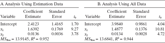
TABLE 11.6 Prediction Performance for the Model Developed from the Estimation Data

where SS_T = 4113.5442 is the corrected sum of squares of the responses in the prediction data set. Thus, we might expect this model to “explain” about 92.2% of the variability in new data, as compared to the 95.2% of the variability explained by the least-squares fit to the estimation data. This loss in R² is small, so there is reasonably strong evidence that the least-squares model will be a satisfactory predictor.

11.3 DATA FROM PLANNED EXPERIMENTS

Most of the validation techniques discussed in this chapter assume that the model has been developed from unplanned data. While the techniques could also be applied in situations where a designed experiment has been used to collect the data, usually validation of a model developed from such data is somewhat easier. Many experimental designs result in regression coefficients that are nearly uncorrelated, so multicollinearity is not usually a problem. An important aspect of experimental design is selection of the factors to be studied and identification of the ranges they are to be varied over. If done properly, this helps ensure that all the important regressors are included in the data and that an appropriate range of values has been obtained for each regressor. Furthermore, in designed experiments considerable effort is usually devoted to the data collection process itself. This helps to minimize problems with “wild” or dubious observations and yields data with relatively small measurement errors.

When planned experiments are used to collect data, it is usually desirable to perform additional trials for use in testing the predictive performance of the model. In the experimental design literature, these extra trials are called confirmation runs. A widely used approach is to include the points that would allow fitting a model one degree higher than presently employed. Thus, if we are contemplating fitting a first-order model, the design should include enough points to fit at least some of the terms in a second-order model.

PROBLEMS

11.1 Consider the regression model developed for the National Football League data in Problem 3.1.

1. Calculate the PRESS statistic for this model. What comments can you make about the likely predictive performance of this model?
2. Delete half the observations (chosen at random), and refit the regression model. Have the regression coefficients changed dramatically? How well does this model predict the number of games won for the deleted observations?
3. Delete the observation for Dallas, Los Angeles, Houston, San Francisco, Chicago, and Atlanta and refit the model. How well does this model predict the number of games won by these teams?

11.2 Split the National Football League data used in Problem 3.1 into estimation and prediction data sets. Evaluate the statistical properties of these two data sets. Develop a model from the estimation data and evaluate its performance on the prediction data. Discuss the predictive performance of this model.

11.3 Calculate the PRESS statistic for the model developed from the estimation data in Problem 11.2. How well is the model likely to predict? Compare this indication of predictive performance with the actual performance observed in Problem 11.2.

11.4 Consider the delivery time data discussed in Example 11.3. Find the PRESS statistic for the model developed from the estimation data. How well is the model likely to perform as a predictor? Compare this with the observed performance in prediction.

11.5 Consider the delivery time data discussed in Example 11.3.

1. Develop a regression model using the prediction data set.
2. How do the estimates of the parameters in this model compare with those from the model developed from the estimation data? What does this imply about model validity?
3. Use the model developed in part a to predict the delivery times for the observations in the original estimation data. Are your results consistent with those obtained in Example 11.3?

11.6 In Problem 3.5 a regression model was developed for the gasoline mileage data using the regressor engine displacement x₁ and number of carburetor barrels x₆. Calculate the PRESS statistic for this model. What conclusions can you draw about the model's likely predictive performance?

11.7 In Problem 3.6 a regression model was developed for the gasoline mileage data using the regressor vehicle length x₈ and vehicle weight x₁₀. Calculate the PRESS statistic for this model. What conclusions can you draw about the potential performance of this model as a predictor?

11.8 PRESS statistics for two different models for the gasoline mileage data were calculated in Problems 11.6 and 11.7. On the basis of the PRESS statistics, which model do you think is the best predictor?

11.9 Consider the gasoline mileage data in Table B.3. Delete eight observations (chosen at random) from the data and develop an appropriate regression model. Use this model to predict the eight withheld observations. What assessment would you make of this model's predictive performance?

11.10 Consider the gasoline mileage .data in Table B.3. Split the data into estimation and prediction sets.

1. Evaluate the statistical properties of these data sets.
2. Fit a model involving x₁ and x₆ to the estimation data. Do the coefficients and fitted values from this model seem reasonable?
3. Use this model to predict the observations in the prediction data set. What is your evaluation of this model's predictive performance?

11.11 Refer to Problem 11.2. What are the standard errors of the regression coefficients for the model developed from the estimation data? How do they compare with the standard errors for the model in Problem 3.5 developed using all the data?

11.12 Refer to Problem 11.2. Develop a model for the National Football League data using the prediction data set.

1. How do the coefficients and estimated values compare with those quantities for the models developed from the estimation data?
2. How well does this model predict the observations in the original estimation data set?

11.13 What difficulties do you think would be encountered in developing a computer program to implement the DUPLEX algorithm? For example, how efficient is the procedure likely to be for large sample sizes? What modifications in the procedure would you suggest to overcome those difficulties?

11.14 If Z isthe n × k matrix of standardized regressors and T isthe k × k upper triangular matrix in Eq. (11.3), show that the transformed regressors W = ZT⁻¹ are orthogonal and have unit variance.

11.15 Show that the least-squares estimate of β (say ) with the ith observation deleted can be written in terms of the estimate based on all n points as

11.16 Consider the heat treating data in Table B.12. Split the data into prediction and estimation data sets.

1. Fit a model to the estimation data set using all possible regressions. Select the minimum C_p model.
2. Use the model in part a to predict the responses for each observation in the prediction data set. Calculate R² for prediction. Comment on model adequacy.

11.17 Consider the jet turbine engine thrust data in Table B.13. Split the data into prediction and estimation data sets.

1. Fit a model to the estimation data using all possible regressions. Select the minimum C_p model.
2. Use the model in part a to predict each observation in the prediction data set. Calculate R² for prediction. Comment on model adequacy.

11.18 Consider the electronic inverter data in Table B.14. Delete the second observation in the data set. Split the remaining observations into prediction and estimation data sets.

1. Find the minimum Cp equation for the estimation data set.
2. Use the model in part a to predict each observation in the prediction data set. Calculate R² for prediction and comment on model adequacy.

11.19 Table B.11 presents 38 observations on wine quality.

1. Select four observations at random from this data set, then delete these observations and fit a model involving only the regressor flavor and the indicator variables for the region information to the remaining observations. Use this model to predict the deleted observations and calculate R² for prediction.
2. Repeat part a 100 times and compute the average R² for prediction for all 100 repetitions.
3. Fit the model to all 38 observations and calculate the R² for prediction based on PRESS.
4. Comment on all three approaches from parts a-c above as measures of model validity.

11.20 Consider all 40 observations on the delivery time data. Delete 10% (4) of the observations at random. Fit a model to the remaining 36 observations, predict the four deleted values, and calculate R² for prediction. Repeat these calculations 100 times. Calculate the average R² for prediction. What information does this convey about the predictive capability of the model? How does the average of the 100 R² for prediction values compare to R² for prediction based on PRESS for all 40 observations?