
Chapter 7
Micro-Image Evaluation
Bloom by Douglas Gaston IV, Biomedical Photographic Communications student, Rochester Institute of Technology
Image Characteristics
The small-scale image characteristics of graininess, sharpness, and detail (collectively called definition) strongly influence picture quality. A photographer can produce a print that has good tone-reproduction qualities but suffers in overall quality because of excessive graininess, lack of sharpness, or insufficient detail. For this reason, it is important to understand small-scale image characteristics and how they relate to the choice of photographic materials, equipment, and processes. The micro-image attributes of sharpness and detail apply to the optical image formed by a lens as well as the photographic image recorded on light-sensitive film or paper. Graininess, however, is a characteristic imposed on the image by the recording material.
Graininess is a subjective property. Granularity is an objective property.
Graininess/Granularity
Photographic emulsions consist of a dispersion of light-sensitive silver halides in a transparent medium such as gelatin. Figure 7-1 represents a small area of unexposed photographic film magnified 2,500 times. Figure 7-1 (A) shows the emulsion in its pristine state, before exposure and development.
The crystals vary in shape and size, and crystals with similar shapes can be oriented in any direction within the thickness of the emulsion. The spacing between the crystals varies, with some crystals touching and others overlapping. Although the crystal size typically varies widely within a given emulsion, the average size is generally larger in fast films than in slow films. It should be noted, however, that the size of the silver halide crystals is not the sole determinant of film speed.
The exposed silver halide crystals are transformed during development into grains of silver that are more or less opaque, depending upon their size and structure (see Figure 7-1 (B)). The developed silver grains seldom conform exactly to the shapes of the silver halide crystals. The size and shape of each silver grain depends upon the combination of exposure, developer type, and degree of development in addition to the size and shape of the original silver halide crystal. As the silver grains increase in size, the spaces between the grains through which light can pass freely become smaller. The overlap in depth of the individual silver grains results in a rather haphazard arrangement of silver grain clusters. This nonhomogeneity of the negative image usually can be detected in prints made at high magnifications as an irregular pattern of tonal variation superimposed on the picture image. Figure 7-2(A) compares enlarged prints and transparencies made from different 35-mm films. Notice the loss of fine detail as graininess increases.
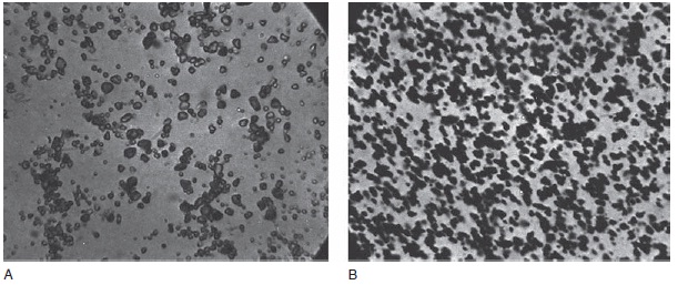
Figure 7-1 Silver halide crystals. (A) Grains of silver halide are randomly distributed in the emulsion when it is made. (B) Silver is developed at the sites occupied by the exposed silver halide.
Graininess is an important variable since it sets an esthetic limit on the degree of enlargement, as well as a limit on the amount of information or detail that can be recorded in a given area of the film. Graininess can be thought of as noise or unwanted output that competes with the desired signal (the image). All recording mediums have some type of noise that limits the faithfulness of the desired signals, including televisions, digital sensors, and video and audio tapes and discs. Graininess, which can be esthetically pleasing, adversely affects sharpness and resolution. Even though graininess, sharpness, and resolution are defined as three distinctly different image characteristics, in practice they are not entirely separate and independent.
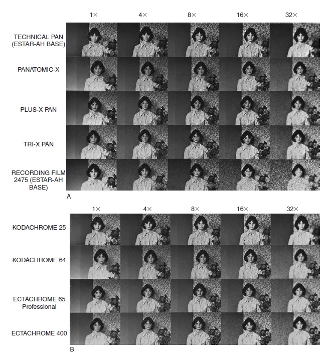
Figure 7-2 The effect of film graininess on detail. (© Eastman Kodak Company.) (A) Comparison prints from five different 35-mm black-and-white negatives at various magnifications. (A 32 X magnification represents a 30 X 45-inch print.) (B) Comparison of four different 35-mm color transparency films at various magnifications (1 X, 4 X, 8 X, 16 X, and 32 X). (Continued on next page.)
Since graininess is generally considered to be an undesirable characteristic, why not make all photographic film fine-grained? Fine-grained film represents a trade-off in which some film speed has been sacrificed. There tends to be a high correlation between graininess and film speed, as shown in Table 7-1. It should be noted, however, that significant advances have been made in emulsion technology so that the fast films of today are much less grainy than they were some years ago. The measurement and specification of graininess have not been standardized internationally because of this caution needs to be exercised when comparing data from different manufacturers.

Figure 7-2 (C) Comparison prints from four different 35-mm color negatives at various magnifications (1 X, 4 X, 8 X, 16 X, and 32 X).
Table 7-1 Comparison of speed and graininess for several panchromatic films intended for pictorial use. (Manufacturers' graininess classifications must be compared with caution since the methods of measurement and specification are not standardized.)
| Film Name | ISO (ASA) Speed | Graininess |
| Plus-X 125 | 125 | Extremely Fine |
| TRI-X 320 (320TXP) | 320 | Fine |
| TRI-X 400 (400TXP) | 400 | Fine |
| T-MAX PS3200 | 3200 | Fine |
| Fuji Neopan1600 | 1600 | Fine |
Graininess tends to increase with film speed, but T-Max 100 and 400 speed films are both rated as having extremely fine grain.
Measuring Graininess
It is relatively simple to look at an enlarged print and determine whether or not graininess can be detected. The extent of the graininess, however, is more difficult to assess. It is tempting to make greatly enlarged prints from two negatives and compare them side-by-side for graininess. Although such a method is commonly used in studies of graininess described in photographic magazines and is appropriate for some purposes, it does not actually measure graininess. It is a subjective qualitative method that enables a photographer to say print A looks grainier than print B, but not to indicate the magnitude of the difference. Even when making such simple comparisons it is difficult to make the prints so that there are no other differences to confuse the issue, such as subject, density, contrast, and sharpness.
Various methods have been used in an effort to obtain a reliable and valid measure of graininess. The most widely used method of measuring graininess directly is a procedure called blending magnification. Under a set of rigidly specified conditions, a negative that has been uniformly exposed to produce a uniform density is projected onto a screen at increasing levels of magnification, beginning at a level where graininess is not visible. A viewer, seated in a specified position with controlled room-light conditions, is asked to determine when graininess first appears. A numerical value is then obtained by taking the reciprocal of the blending magnification and multiplying it by 1,000. For example, if the blending magnification is 8, then 1/8 X 1,000 = 125. The number 125 represents the graininess of that negative under the conditions specified, and as the conditions are repeatable, other negatives could be so measured.
A practical alternative to the blending magnification method is to keep the magnification constant but to vary the viewing distance. One can move toward a print until it begins to look grainy. The minimum distance at which graininess is not evident is the blending distance, and the number is a measure of graininess. Such blending distance measurements, although practical, are subject to variability.
How a print is going to be viewed must be considered when judging the amount of grain visible. One does not normally view a 16 X 20-inch print at a reading distance of 10 inches, nor an 8 X 10-inch print at a distance of 10 feet. How the final print will be viewed or reproduced is important. Photographs reproduced in newspapers using a 60 lines/inch screen will look grainier than those reproduced in a quality magazine using a 150 lines/inch screen. Motion pictures present an interesting situation, since each frame is in the projector gate for only 1/24 second. When one views a motion picture at a large magnification, as from the front row in a theater, graininess is commonly experienced as a boiling or crawling effect, especially in areas of uniform tone. This is a result of the frame-to-frame change of grain orientation.
It is essential that the density level be specified when making graininess measurements. As shown in Figure 7-3, graininess highly depends upon the density level. With negatives, maximum graininess occurs at a density between 0.3 and 0.6, depending to some extent upon the luminance level of the test field. A density of 0.3 corresponds to a transmittance of one half, which represents equal clear and opaque areas. One would expect little graininess at very low and very high density levels, but for different reasons. At very low densities there is little grain structure. As the density of the negative increases, the amount of light transmitted decreases. The perception of graininess decreases rapidly as the density increases because our ability to see detail and tonal differences decreases at low light levels,.
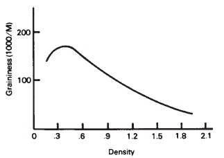
Figure 7-3 Negative graininess is highest at a density of 0.3 to 0.6 and then decreases rapidly as density increases. (The illuminance on the sample is constant.)
At a very high density, graininess is not perceptible even though the silver in the negative has a very grainy structure. This can be demonstrated by selecting a negative having a uniform density of about 1.5 and increasing the intensity of the viewing light source 16 times. The appearance of graininess will jump considerably, for in effect the density of 1.5 behaves as though it were a density of only 0.3 with respect to viewing luminance. In fact, if the light level is adjusted so that the transmitted light remains constant regardless of the density level, the result will be the curve shown in Figure 7-4, which indicates that the graininess increases gradually with increasing density.
When comparing prints or negatives for graininess, the prints or negatives should match in density, contrast, and sharpness.
Graininess is most easily detected in uniform midtone areas. Condenser enlargers increase graininess.
There is another method of demonstrating that graininess increases with negative density when compensation is made for the lower transmittance that involves making a series of photographs of a gray card with one-stop variations of exposure, from four stops below normal to four stops over. Developing the film normally will produce negatives having nine different density levels ranging from about 0.2 to about 1.5. Each negative is printed at a fixed high magnification with the necessary adjustment in the printing exposure time to produce the same medium gray density on all of the prints. The prints should be viewed side-by-side under uniform illumination and at the same distance to observe differences in graininess.
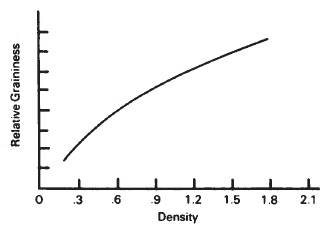
Figure 7-4 Graininess increases as density increases if the light reaching the eye is adjusted so that it is the same regardless of the density of the negative.
Considerable variation in the density level at which graininess is most apparent has been found among different types of images such as film negatives, prints, projected black-and-white transparencies, projected color transparencies, black-and-white television, and color television. The density level is higher for color images than for black-and-white, for transparencies as well as television, as shown in Figure 7-5. This is partly due to the scattering of light by silver particles, known as the Callier effect. The Callier coefficient, a measure of this effect, is the ratio of the density with specular illumination to the density with diffuse illumination. Since color dyes scatter the light very little, the Callier coefficient is approximately 1.0 with color images. In black-and-white images, the scattering of light and the Callier coefficient increase with density and the size of the silver grains, producing values higher than 1.0.

Figure 7-5 The density at which graininess is most objectionable is different for black-and-white and for color films, and for different systems of projection. (The difference between black-and-white and color is due mostly to the Callier Q factor—silver images scatter more light.) (Redrawn from Zwick, D., "Film Graininess and Density: A Critical Relationship," Photographic Science and Engineering 16:5 (1972), p. 345.)
Recent measurement of graininess for black-and-white and color prints reveals that the black-and-white prints exhibit peak graininess at a density of about 0.65 and color prints at an average density of about 0.93, with some prints peaking at a low density of 0.80 and others at a high density of 1.05. Further, it was found that varying the level of illumination on prints had little effect on the density at which peak graininess was observed. “An increase in illumination level by a factor of 6.5X increases the critical density by about 0.07. The shift in critical density that would occur between viewing a print in sunlight and with indoor home lighting would be less than 0.2 density."1 (The illumination level does of course have a pronounced effect on the perceived tone reproduction of a print.)
Grain Size and Image Color
Although we think of the silver image as being black, as the term black-and-white implies, the color can vary considerably between images depending upon the size and structure of the silver particles. Large silver particles absorb light almost uniformly throughout the visible spectrum, producing neutral color images that appear black where the density is high. Smaller silver grains absorb relatively more light in the blue region than in the green and red regions, causing the images to appear more brownish. By making the silver particles sufficiently small, it is possible to obtain a saturated yellow color, as exemplified by the yellow filter layer between the top two emulsion layers in some color films.
When the smallest dimension of small particles approximates the size of the wavelength of light, they scatter light selectively by wavelength, an effect known as Rayleigh scattering. Since the scattering varies inversely with wavelength to the fourth power, blue light is scattered most, and the transmitted light appears reddish. Finegrained negatives that have a brownish color can have different printing characteristics than would be predicted by visual inspection, because of the lower Callier coefficient when printing with a condenser enlarger, and because of the different response of some printing materials to light of different colors— for example, variable-contrast papers.
Granularity
Controlled graininess can be used to create a textured or impressionistic effect. Granularity is the objective measure of density non-uniformity that corresponds to the subjective concept of graininess. Granularity determination begins with density measurements made with a microdensitometer (a densitometer that has a very small aperture) across an area of a negative that has been uniformly exposed and developed. The data are automatically recorded and mathematically transformed into statistical parameters that can be used to describe the fluctuations of density due to the distribution of the silver grains in the negative, and therefore to determine the granularity.
The process can be described graphically as illustrated in Figure 7-6. The fluctuations are greater at a density of 1.0 than they are at a density of 0.3. If all of the many points indicating the variation from an assumed average density are collapsed as shown on the left of the illustrations, a near-normal distribution is generated. Such a curve allows the specification of granularity in statistical terms that may be generalized. For any mean or average density (D), the variability of density around that mean is specified by the standard deviation a (D) (read sigma D). Because a (D) is the root mean square (rms) of the deviations, such granularity measurements are called rms granularity. (Root mean square is the standard deviation of micro-density variations at a particular average density level.)

Figure 7-6 Microdensitometer traces of a negative material at a high density and at a low density. The fluctuation of density over micro-areas on the negative describes the granularity of the negative. The higher density of 1.0 has greater fluctuations and therefore higher granularity.
The best way to minimize graininess is to use a fine-grain film.
Granularity values for Kodak negative films, and reversal and direct duplicating films are made at a density of 1.00. Microdensitometer traces are made with a circular aperture having a diameter of 48 micrometers (0.048 mm).
Since there is a good correlation between granularity measurements and graininess, rms granularity numbers are used to establish the graininess classifications found in some data sheets and data books: microfine, extremely fine, very fine, fine, medium, moderately coarse, coarse, and very coarse grain. In addition to providing a good objective correlate for graininess, rms granularity is analogous to the way noise is specified in electronic systems. This provides an important linkage for photographic-electronic communication channels and systems. Some typical values of rms granularity for several Kodak films and plates are shown in Table 7-2. They were made with a microdensitometer having a scanning aperture of 48 micrometers, corresponding to a magnification of 12, on a sample having a diffuse density of 1.0.
Kodak has also adopted the KODAK Grain Index. This method replaces the rms granularity value and cannot be compared to rms values. This method is referred to as the Print Grain Index (PGI) and is designed to be more meaningful to a photographer who is accustomed to viewing prints rather than a negative. The PGI utilizes a perceptual scale, equating a two unit change to equal one just noticeable difference (jnd) in graininess. A value of 25 on this scale represents the visual threshold for graininess. A higher value would indicate an increase in the amount of viewable grain. This scale was designed using prints made off a diffusion enlarger and may not be accurate for other printing systems. Other manufactures have developed similar systems.
Table 7-2 Some Kodak films and their rms granularities. The data represent a very specific set of conditions of testing. Any comparison of rms granularity for other films must be made under the same set of conditions
| Film Name | Diffuse rms Granularity |
| Plus-X 125 | 10 |
| TRI-X 320 (320TXP) | 16 |
| TRI-X 400 (400TXP) | 17 |
| T-MAX PS3200 | 18 |
Minimizing Graininess
Much has been written and claimed about developers for reducing graininess. The same could be said for such claims as was said years ago by Mark Twain when he read his obituary in a newspaper: “Claims are highly exaggerated." Two major problems with claims of reduced graininess are the questionable authenticity of the testing procedures and the failure to completely report difficulties and losses associated with such reduction. Validity of graininess comparison tests requires negatives that have been exposed and developed to produce the same density and contrast, and printed to produce the same tone reproduction. This is a difficult task, and processing the film for the manufacturer's recommended time and temperature seldom produces negatives that meet these requirements. The fact of the matter is that little can be done to improve graininess through development unless one is willing to sacrifice one or more other attributes such as film speed, image sharpness, and tone-reproduction quality. Depending upon the requirements for specific photographic situations, such trade-offs may be warranted, but there is no substitute for beginning with a fine-grained film.
Fine-grain development always results in a loss of film speed. In situations where minimum graininess and maximum film speed are both important, the photographer is presented with a choice of using a high-speed film and a fine-grain developer or a slower film that has finer inherent grain with normal development. The control over graininess by the choice of developer tends to be small compared to the control by the choice of film. Films that are especially designed for microfilming, where high contrast is appropriate and slow speed is tolerable, have a low level of graininess that is truly remarkable. Such films have even been used for pictorial photography by developing them in low-contrast developers in situations where the lack of graininess is a more important consideration than the slow speed.
Graininess of Color Films
Color films exhibit graininess patterns having both similarities and differences, compared with the graininess patterns in black-and-white films. With dye-coupling development, dye is formed in the immediate area where a silver image is being developed so that the dye image closely resembles the grain pattern of the silver image, and the dye pattern remains after the silver image is removed by bleaching. The image structure is more complex with color film due to the three emulsion layers, each containing a different color-dye image. Graininess and granularity are measured and specified in the same manner with color films as with black-and-white. The perception of graininess with color films results from the luminosity (brightness) contribution of the three dye images rather than from the hue and saturation attributes, although the appearance of graininess is not equal for the three colors. The relative contribution of each of the dye layers to granularity is as follows:
|
Green record |
(Magenta dye layer) |
60% |
|
Red record |
(Cyan dye layer) |
30% |
|
Blue record |
(Yellow dye layer) |
10% |
These percentages will vary depending upon the dyes used, but the magenta layer will always be the major contributor to the perception of graininess, mainly because our eyes are most sensitive to green light, which the magenta dye layer controls. Figure 7-2(B) compares four different 35-mm color-transparency films at various magnifications while Figure 7-2(C) compares prints made from four different 35-mm color negatives at various magnifications (1X, 4X, 8X, 16X, and 32X).
Sharpness/Acutance
Textured paper surfaces obscure graininess.
In art, the terms hard-edged and soft-edged are sometimes used to describe the quality of an edge in an image. In photography the term sharpness describes the corresponding abruptness of an edge. Sharpness is a subjective concept, and images are often judged to be either sharp or unsharp, but sharpness can be measured. If one photograph is judged to be sharper than another, the sharpness is being measured on a two-point ordinal scale. If a large number of photographs are arranged in order of increasing sharpness, the sharpness is being measured on a continuum on an ordinal scale.
Sharpness and contrast go hand-in-hand.
The sharpness of a photographic image in a print is influenced and limited by the sharpness characteristics of various components in the process, including the camera optics, the film, the enlarger optics, and to a lesser extent the printing material. Sharpness and contrast are closely related, so any factor that increases image contrast tends to make the image appear sharper. Similarly, anything that decreases image sharpness, such as imprecise focusing of the enlarger, tends to make the image appear less contrasty.
Glossy print surfaces enhance contrast and sharpness.
Although it is not possible to obtain a sharp print from an unsharp negative simply by focusing the image with an enlarger, there are various procedures available for increasing the sharpness of photographic images. Some film developers, for example, produce higher local contrast at the boundaries between areas of different density, which causes the image to appear sharper. The anomaly on the denser side of the boundary is called a border effect, the anomaly on the thinner side is called a fringe effect, and the two together are referred to as edge effects. There are also electronic and photographic techniques for either making an image edge more abrupt or increasing the local contrast at the edge.
Developing factors that alter edge effects, and therefore image sharpness, include developer strength, developing time, and agitation. Diluting the developer and developing for a longer time with little or no agitation enhances edge contrast and sharpness. Unfortunately, this procedure can also cause uneven development with some film-developer combinations even though it is used routinely with high-contrast photolithographic materials. One developer specifically formulated to enhance image sharpness with nor-mal-contrast films is the Beutler High-Acutance Developer, named after the man who pioneered developers of this type. The formula is:
|
Sodium sulfite (Na2SO3) |
5.0 g |
|
Metol |
0.5 g |
|
Sodium carbonate (Na2CO3) |
5.0 g |
|
Water |
1 liter |
Acutance
Acutance is a physical measurement of the quality of an edge that correlates well with the subjective judgment of sharpness. It is measured in a laboratory by placing an opaque knife edge in contact with the photographic material being tested and exposing the material with a beam of parallel (collimated) light. This produces, after development, a distinct edge between the dense and clear areas, but because of light scatter in the emulsion the edge has a measurable width. The edge, which is less than 1 mm (1,000 microns) wide, is then traced with a microdensitometer. The result is a change in density with distance. A typical density-distance curve is shown in Figure 7-7. The rate at which density changes as a function of the microdistance of the edge is a graphical description of acutance (sharpness).
The rate of change of density can be expressed in terms of slope or gradient. The average gradient of the curve between two specified points becomes a numerical expression of acutance, as shown in Figure 7-8. Cutoff points A and B establish the part of the curve over which the geometric average gradient will be determined. The gradient AD/Ax is found for each of the intervals between A and B. The gradients are then squared, and the squared gradients are added together and divided by the number of intervals to determine the average square gradient. The formula for these calculations is provided in Equation 7-1:
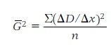 (Eq. 7-1)
Figure 7-7 The rate at which the density changes across the edge of an image is described by the slope of the curve. The film represented by curve 1 has a higher slope or gradient and therefore has higher acutance and sharpness.

Figure 7-8 To obtain a numerical value for acutance, the average gradient of the curve is calculated and then divided by the density scale (DS).
Acutance is calculated by dividing the average square gradient by the density scale (DS) between points A and B on the vertical scale as shown in Eauation 7-2:
Resolving Power
Resolving power is the ability of the components of an image-formation process (camera lens, film, projector lens, enlarging lens, printing material, etc.) individually or in combination to reproduce closely spaced lines or other elements as separable. Resolving power is the correlate of the image quality referred to as detail, so that a lens having high resolving power is capable of reproducing fine detail. Targets used to measure resolving power typically have alternating light and dark elements either in the form of parallel bars as in the United States Air Force (USAF) or American National Standards Institute (ANSI) Resolution Targets (see Figure 7-9). Test targets are commonly supplied in high-contrast (black-and-white) and lower-contrast forms because subject contrast influences resolving power.
Alphanumeric resolution targets produce less variability among observers
Resolving power and film speed tend to vary inversely.

Figure 7-9 Examples of two resolution test targets. Although the USAF and the ANSI targets look different, they are quite similar. Both take the shape of a spiral made up of three black bars that have a square format and decrease in size (increase in line frequency). The USAF target has both vertical and horizontal bars, which allows a check for astigmatism. The ANSI target would have to be rotated 90 degrees and photographed twice to accomplish the same thing.
To test the resolving power of a lens, a target is placed on the lens axis at the specified distance (for example, 21 times the focal length) to produce an image at a specified scale of reproduction (for example, 1/20). The aerial image is examined with a microscope at a power about equal to the expected resolving power, and the finest set of lines or elements that can be seen separately is selected. A conversion table translates this information into lines-per-millime-ter resolving power, usually in terms of dark-light pairs of lines. Alternative methods of expressing resolving power are in lines-per-unit-distance in object space rather than in the image, and as angular resolving power.

Figure 7-10 Resolution test targets arranged to measure resolving power on and off axis.
Variations can be made in the above procedure to obtain additional information. A row of targets can be used so that the images fall on a diagonal line at the film plane to determine the resolving power for various off-axis angles as well as on-axis (see Figure 7-10). The test can be repeated with the lens set at different f-numbers to determine the setting that provides the best compromise between reducing lens aberrations and introducing excessive diffraction. The effect of filters on the optical image can be determined by measuring the resolving power with and without the filter, also with and without compensation for focus shift with the filter.
The relationship between the resolving power of the components of a system and the resolving power of the entire system is commonly expressed with the formula 1/R = 1/r1 + 1/r2 + 1/r3 … where R is the resolving power of the system and each rn is the resolving power of each component in the system. This formula reveals that the resolving power of the system cannot be higher than the lowest resolving power component. In fact, the resolving power of the system is always lower than the lowest component. If, for example, a lens with a resolving power of 200 lines/mm is used with a film having a resolving power of 50 lines/mm, the resolving power of the combination is 40 lines/mm. Thus it would be a mistake to believe that the quality of the camera lens is unimportant for photographs made for reproduction in newspapers and on television, where the maximum resolving power is relatively low. The only question is whether differences in resolving power of two lenses would produce a noticeable difference in the reproduction.
Since it is not possible to measure the resolving power of photographic film directly, it is common practice to use the film with a high-quality lens of known resolving power, determine the resolving power of the system, and then calculate the film's resolving power. The resolving power of the lens-film combination is referred to as photographic resolving power to distinguish it from film resolving power and lens resolving power.
Resolving-Power Variables
A number of factors can enter into the testing procedure to produce variable resolving-power values, including the following:
Test target contrast. The higher the contrast of the test target, the higher the measured resolving power will be. Black-and-white reflection targets have a luminance ratio contrast of approximately 100:1. The ratio for low-contrast targets may be as low as 2:1 or even less. The transmittance ratio for transparency test targets is generally about 1,000:1. High-contrast and low-contrast test targets are illustrated in Figure 7-11, and comparison data for the two types are presented in Table 7-3.
Focus. Focusing inaccuracies can be caused by human error or mechanical deficiencies. With lenses having residual curvature of field, the position of optimum focus will not be the same for on-axis and off-axis images. Other common problems are a difference between the position of the focusing screen and the position of the film plane, and film buckle. Bracketing the focusing position is sometimes advisable.

Figure 7-11 High-contrast and low-contrast resolving-power test targets. The target on the top has a contrast ratio of 100:1, while the one on the bottom is 2:1 with the correct exposure.
The resolving power of a film is higher when measured with a high-contrast test target.
Camera movement. Any movement of the camera during exposure will have an adverse effect on resolving power, including the jarring caused by mirror movement in single-lens reflex cameras.
Exposure level. There is an optimum exposure level, with a given film, to obtain maximum resolving power. This level does not necessarily correspond to the published film speed.
Resolving power changes with exposure, and is highest with the correct exposure.
Table 7-3 Resolution, word, and numerical data for several Kodak films. In general, as the speed of the film increases, resolution decreases. Resolution measured with a high-contrast target is two or more times that measured with a low-contrast target. (Special films such as spectroscopic plates have resolution values up to 2,000 lines/mm but speed values of about 1.0 or less.)
| Resolution in Lines/mm | ||||
| Kodak Film | (ASA) Speed | Low Contrast | High Contrast | Resolution Word Category or H.C. |
| T-MAX 100 | 100 | 62 | 200 | Very High |
| Plus-X | 125 | 50 | 125 | High |
| T-MAX 400 | 400 | 50 | 125 | High |
Development. The degree of development affects negative density, contrast, and granularity, all of which can influence resolving power.
Light source. Exposures made with white light and with narrow-wavelength bands of light, ultraviolet radiation, or infrared radiation can produce different resolving-power values for a variety of reasons including chromatic aberration, diffraction, and scattering in the emulsion.
Table 7-4 Resolution values from six outstanding photographic organizations testing the same film under the same specified conditions. The upper values represent raw data while the lower values are rounded off to fit categories specified by ANSI

Human judgment. Different viewers may disagree on which is the smallest set of target lines that can be resolved in a given situation. With experience, a person can become quite consistent in making repeated interpretations of the same images. For this reason, resolving power is more useful for comparison tests made by one person than in comparison tests of resolving-power values to published values. Table 7-4 shows the variations in resolving power when six different laboratories tested the same film using high-contrast, medium-contrast, and low-contrast targets. The values represent an average of three tests for each condition. The upper table shows the results before the numbers were rounded off to fit the established ANSI categories. Much of the variation can be attributed to the difficulty viewers have in judging which set of lines is just resolvable.
“The resolving power of a photographic material is not measurable apart from the other components of the photographic process. What we invariably estimate is the resolution of a system, including the target, the illumination method, the optical system, the photographic material and its treatment, and the readout method."2 The same can be said in testing resolution for any system—the resolution of paper copies made on machines such as Xerox, and IBM machines; the resolution of video systems; the resolution of printing plates used in graphic arts printing; the resolution of the human eye; and so on.
Resolving-Power Categories
Since resolving-power numbers mean little to those who are inexperienced in working with them, words are sometimes used to describe resolving-power categories. Eastman Kodak Company has set up the following relationship between words and numbers for films:
|
Ultra high |
630 lines/mm and higher |
|
Extremely high |
250, 320, 400, 500 lines/mm |
|
Very high |
160, 200 lines/mm |
|
High |
100, 125 lines/mm |
|
Medium |
63, 80 lines/mm |
|
Low |
50 lines/mm and below |
Resolving Power And Graininess
The effect of graininess on resolution can be seen in Figure 7-12. The sequence of prints are of a person and a resolution target photographed simultaneously at three increasing distances between subject and camera. All three photographs were made on the same 35-mm film and processed at one time. To obtain the same image size, different amounts of enlargement were required. The first print can be considered normal. Notice that there is detail and texture in the woman's coat and that many of the pine needles are easily distinguishable. Similarly, fine detail is maintained in the resolution target as seen in the small distinguishable lines in the center array. In the second and third prints the fine detail in both pictures has been increasingly obscured by the increase in graininess. The fine detail in the woman's coat, her facial features, the pine needles, and the small bars in the resolution target are no longer distinguishable. The coarser areas of the photograph, however, are still distinguishable as seen by the large array of three-bars and the solid black square in the resolution target, and the vertical black area of the woman's coat. Graininess, which is the major contributor to visual noise in a photographic system, takes over and the signal (information) is diminished or completely lost.
Resolving power is not a dependable indicator of the appearance of relative sharpness of images.
Land resolution from an orbiting satellite is approximately 20 meters per line pair from a height of about 400 miles.
Resolving Power And Acutance
Although image detail and sharpness are commonly perceived as similar, and the corresponding measurements of resolving power and acutance often correlate well, they can vary in opposite directions. That is, one film or lens can have higher resolving power but lower acutance than another film or lens. There was some dissatisfaction with the heavy reliance on resolving power used as a measure of image quality in the past because occasionally a photograph that tested higher in resolving power than another photograph was judged by viewers to be inferior in small image quality. A small loss of fine detail, which corresponds to a reduction of resolving power, may be less objectionable esthetically than a loss in sharpness or contrast (see Figure 7-13).

Figure 7-12 The effect of graininess on resolving power. 4 X magnification. 16 X magnification. 32 X magnification. (Photographs by Carl Franz.)
Graininess tends to lower film-resolving power.
When trying to obtain a reliable and valid measure of image quality, it is tempting to search for a single number that will describe that characteristic. As early as 1958, two research scientists, George C. Higgins and Fred H. Perrin, cautioned: “No single number can be attached to any system to describe completely its capability of reproducing detail clearly."3
Modulation Transfer Function (MTF)
The modulation transfer function is a graphical representation of image quality that eliminates the need for the observer to make decisions. The MTF system differs from resolving-power measurement in two other important ways. First, the test object generates a sine-wave pattern rather than the square-wave pattern generated by a resolving-power target; second, the percent response at each frequency is obtained. Resolving-power values are threshold values, which give only the maximum number of lines resolved—that is, the highest frequency. Figure 7-14 shows a sine-wave test target, a photographic image of the target, and a microdensitometer trace of the image. Note that the test target increases in frequency from left to right and that the “bars" do not have a hard edge but rather a soft gradient as one would expect from a sine wave.
The modulation transfer function is a graph that represents the image contrast relative to the object contrast on the vertical axis over a range of spatial frequencies on the horizontal axis, where high frequency in the test target corresponds to small detail in an object. If it were possible to produce a facsimile image, the contrast of the image would be the same as the contrast of the test target at all frequencies, and the MTF would be a straight horizontal line at a level of 1.0. In practice, the lines always slope downward to the right, since image contrast decreases as the spatial frequency increases. Eventually the lines reach the baseline, representing zero contrast, when the image-forming system is no longer able to detect the luminance variations in the test target. As with resolving power, an MTF can be determined for each component in an image-forming system or for combinations of components. The MTF for a system can be calculated by multiplying the modulation factors of the components at each spatial frequency.

Figure 7-13 Enlargements of small images of a test object made on the same film. The left image was made on the optical axis of the lens where acutance was high but resolving power was low. The right image was made 15° to the right of the optical axis where the acutance was low but resolving power was high.
The advantage of modulation transfer functions is that they provide information about image quality over a range of frequencies rather than just at the limiting frequency as does resolving
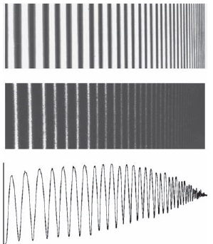
Figure 7-14 To measure modulation transfer functions a sinusoidal test target is photographed and then a microdensitometer trace made of the photographic image. (© Eastman Kodak Company.) (Top) Sine-wave test target. (Middle) Photographic image of test target. (Bottom) Microdensitometer trace of the photographic image of the test target.
power; but there are also limitations and disadvantages. For example, photographers cannot prepare their own modulation transfer functions, and the curves are more difficult to interpret than a single resolving-power number. MTFs are most useful for comparison purposes. Figure 7-15 shows published curves for two pictorial-type films having speeds of 32 and 1250. Although both films have the same response up to about 5 cycles/mm, the response falls off more rapidly for the faster film as the frequency increases, indicating that the slower film will hold fine detail better. It should be noted also that modulation transfer functions for lenses do not provide the desired information about off-axis aberrations such as coma and lateral chromatic aberration. When this information is needed, it is necessary to go through an additional procedure to produce an optical transfer function.
The following is an example of how a system MTF can be determined by multiplying the modulation factors of the components. If the modulation factors at 50 cycles/mm are 0.90 for the camera lens, 0.50 for the film, 0.80 for the enlarger lens, and 0.65 for the printing paper, the product of these numbers, and therefore the modulation factor for the system, is 0.23.
Definition is a broad term that includes sharpness, detail, and graininess.
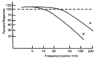
Figure 7-15 MTF curves for two pictorial films with quite different film speeds. Film A is a slow film (ISO 32) and B is a fast film (ISO 1250). One could expect intermediate speeds to fall between A and B. (Output values greater than 100% are the result of adjacency effects in the film.)
Photographic Definition
Photographic scientists and engineers stress the fact that no single number satisfactorily describes the ability of a photographic system to reproduce the small-scale attributes of the subject. The term definition, however, is used to describe the composite image quality as determined by the specific characteristics of sharpness, detail, and graininess (or the objective correlates acutance, resolution, and granularity). Definition is applied to optical images, as well as images recorded on photographic materials, although the term optical definition is preferred for the former and photographic definition is preferred for the latter. The modulation transfer function was introduced as a more comprehensive objective measure of image quality since the measured resolving power of a photographic lens, material, or system did not always correlate well with perceived image definition. Because it is difficult to translate modulation transfer function curves into small-scale image quality, photographers have still felt the need for a simple but meaningful measure of definition. One film manufacturer has attempted to satisfy this need by rating its films on the basis of the degree of enlargement allowed, which takes into account the combined characteristics of graininess, sharpness, and detail.
It should be noted that photographic definition is not determined entirely by the quality of the photographic lens and the photographic materials, but also by factors such as focusing accuracy, camera and enlarger steadiness, subject and image contrast, exposure level, and use of filters. It is not realistic to demand the same level of definition for all types and uses of photographs, including exhibition photographs, motion-picture films, portraits, catalog photographs, and photographs to be reproduced in magazines, newspapers, and on television. Many publications refused to accept black-and-white or color photographs made with small-format cameras long after it had been demonstrated that such cameras were capable of making photographs with better definition than the photomechanical processes were capable of reproducing.
Pixels
In digital photography, a light-sensitive, electrically-charged microchip (either a CCD, CMOS or Foveon X3) serves as the equivalent of film in a camera. Silicon is generally used as a light-sensitive surface and the chip is designed as a rectangular mosaic containing hundreds of thousands of discrete minute areas that act as photoreceptors. Each area is capable of registering picture information and is called a pixel (picture element). (A microchip is also analogous to the retina of the eye, which contains a mosaic of minute light-sensitive receptors called rods and cones, or simply photoreceptors.) Figure 7-16 illustrates a light-sensitive silicon chip. For reproduction purposes only 400 receptors or pixels are shown, whereas in reality they contain as many as half a million pixels within a one-half-inch square area. As light falls on the chip, each pixel generates electrical signals that are proportional to the illuminance. The signals from each pixel are transmitted to a magnetic recording disk. The magnetic image can then be converted to a positive or negative image to be viewed on a monitor or printed on paper to form a “hard copy.”
Figure 7-16 A representation of a silicon charge-coupled device (CCD) with 400 squares or pixels. The camera's lens focuses the image of an object or scene on the many light-sensitive discrete surfaces (pixels) of a CCD. The CCD converts the image into an array of electrical charges that are proportional to the intensity of the light falling on each pixel (light-sensitive square).
To specify and compare the image-quality capabilities of a light-sensitive microchip, the term pixel is used. The greater the number of separate or discrete pixels possible per unit area of a chip, the higher the potential image quality. Put differently, the smaller the pixels, the more pixels per unit area, and the better the image quality. One way to compare the image-quality potential of a microchip system to a photographic system or other system of picture recording, such as television and graphic arts printing, is in terms of point spread functions, described earlier. The smaller the point spread function of a pixel, the more information that can be packed per unit area.
With this in mind, imagine the 400-pixel chip in Figure 7-16 as having 1,000 pixels within each of the 400 small squares shown.
Pixel means picture element.
Further imagine the overall square being reduced to an area of one-half square inch. This would provide a microchip having 400,000 pixels. Each pixel would be about 0.0008 inch in diameter (about half the diameter of a human hair). In 1983 a one-half-inch-square chip (12.7 X 12.7 mm)—about the size of a fingernail—had a total of about 280,000 pixels. By comparison, Kodacolor film of about the same size used in the 1982 disk camera had a total of about 3 million pixels, each pixel being about 0.0003 inch in diameter. With photographic emulsions, the number of pixels possible per unit area is determined by the granularity and acutance of the emulsion. Current high-end digital camera can have over 21 million pixels present. As a comparison, the human eye contains about 127 million pixels consisting of 120 million rods and 7 million cones all contained in an area about 2 inches square (see Figure 7-17). The cones are much smaller than the rods, the smallest cone receptor being about 0.00008 inch (2 micrometers) in diameter.
Figure 7-17 The 120 million rods and 7 million cones in the retina of the human eye can be thought of as a total of 127 million pixels.
Common to all systems of picture recording is the breaking up of a larger continuous optical image into small discrete elements. In photography the discrete picture elements are played back optically, whereas with silicon microchips the information is played back electronically. Since the pixels are discrete photoreceptors, they provide a digital system of recording and playback of pictorial information, as well as text information.
In new micrographic technology, laser beams focused to about one-half micron are used to imprint information on a light-sensitive optical disk as tiny pits or holes. These pixels can be packed closely enough to record the images of 10,000 letter-size documents on a 12-inch-diameter disk.
On a television screen, the individual areas of the phosphors can be thought of as pixels. In the United States, a conventional 525-line television screen consists of 49,152 pixels, 256 in the horizontal direction and 192 vertically (see Figure 7-18). (In Europe a 625-line screen is common. High-resolution screens have about
Figure 7-18 Television phosphors as pixels (enlarged view).
1,000 lines.) This provides the level of picture quality seen on broadcast television. A much better picture is available, however, with a TV monitor, which consists of 128,000 pixels (640 X 200), or with higher-resolution monitors such as those with 262,144 pixels (512 X 512). In general, the more pixels per unit area of screen, the better the picture quality (Figure 7-19). There is presently no generally agreed-upon terminology for specifying the resolution of computer-generated images in terms of the number of discrete pixels. However, a qualitative grouping, as shown in Table 7-5, can be helpful. An illustration of the letter A on a low-, medium-, and high-resolution computer slide-generating system is shown in Figure 7-20.
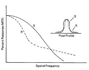
Figure 7-19 Response curves for two hypothetical television tubes. The information displayed by tube S will appear sharper but will have less resolution than that of tube R.
Table 7-5 Arbitrary grouping of pixels in terms of resolution
| Computer-Generated Images Resolution | ||
| Pixels | Total Pixels | Resolution Category |
|
250 X 250a |
62,500 | Low |
| 500 X 500 | 250,000 | Medium |
| 2,000 X 2,000 | 4,000,000 | High |
|
4,000 X 4,000b |
16,000,000 | Very High |
a On a 19-inch diagonal TV screen, each pixel would have a diameter of about 1/16 inch.
b Kodak Ektachrome films can resolve about 3,000 X 4,500 pixels in 35-mm format (1 inch X 11/2 inches) for a total of 13,500,000 pixels. Each pixel would have a diameter of about 0.000.001 (one millionth of an inch).
Digital Resolution
Many of the factors that affect the resolution of a film system also affect the resolution of a digital system. Other additional factors to consider include the number of pixels available and the system electronics that may be altering the digital data by applying image compression or gamma correction. The ISO has established a standard for determining the resolution of a electronic still-picture cameras (ISO 12233). The ISO calls for all resolution measurements to be performed in the digital domain employing digital analysis techniques.
Figure 7-21 illustrates the target that the ISO has specified for use with digital cameras. The target is illuminated at 45° angles from both sides and an exposure made so that the white of the target is near the maximum digital count and there should be no clipping of digital counts in either the white or black areas of the target.
A visual resolution measurement may be made displaying the image on a monitor or creating a hardcopy image. Care must be taken that the monitor or printer have higher resolution than the camera. Magnification on a monitor is allowed. A spatial frequency response may also be calculated from the target using image processing software.
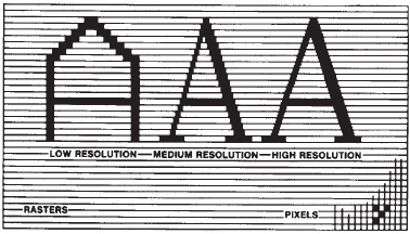
Figure 7-20 This illustration simulates the letter quality obtained by low-, medium-, and high-resolution computer slide-generating systems. (Illustration courtesy of Professor Deane K. Kayton, Audio-Visual Center, Indiana University.)
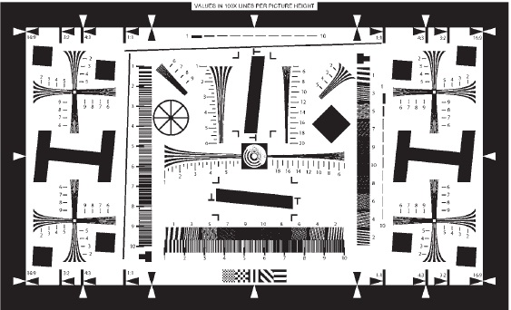
Figure 7-21 Resolution target for electronic still cameras
T-Grain Emulsions
Major advancements in the field of emulsion chemistry have led to films with significantly increased film speed and no loss of sharpness or increase in graininess. In 1982, Eastman Kodak announced a major breakthrough in emulsion technology with their new T-grain emulsion. Figure 7-22 compares a conventional-grain emulsion with the T-grain emulsion at a magnification of 6,000 X. (An electron microscope was used, as optical microscopes are limited to magnification of about 850 X.) Notice that the conventional grains are pebbleshaped whereas the T-grains are flat and present a larger surface per unit volume, which maximizes absorption of incoming incident light. The result is a much faster film with about the same amount of silver and no loss in image quality.
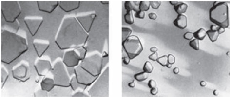
Figure 7-22 Silver halide grains at 6,000 X magnification. The T-grains appear flat and absorb light more efficiently than the conventional pebblelike grains to the right.
REVIEW QUESTIONS
- The general term that includes sharpness, graininess, and detail is …
- acutance
- tone reproduction
- definition
- resolution
- Graininess is most evident in the areas of a print having …
- a uniform light tone
- a uniform medium tone
- a uniform dark tone
- high-contrast fine detail
- Some fine-grain silver images appear warm in color because the small particles of silver …
- transmit red light
- oxidize and turn reddish
- scatter short wavelength light
- Granularity is determined by means of calculations based on …
- blending magnification
- blending distance
- microdensitometer densities
- the number of grains per square millimeter
- Acutance is an objective term that corresponds to the subjective term …
- detail
- sharpness
- graininess
- definition
- localization
- Resolving power is an objective term that corresponds to the subjective term …
- detail
- sharpness
- definition
- recognition
- detection
- If a camera lens has a resolving power of 200 lines/mm and film has a resolving power of 100 lines/mm, the resolving power of the combination is …
- 50 lines/mm
- 67 lines/mm
- 100 lines/mm
- 200 lines/mm
- 300 lines/mm
- Modulation transfer function graphs represent the relationship between …
- subject density and image density
- image exposure and image density
- subject contrast and image contrast
- subject resolving power and image resolving power
- It is estimated that the retina of the human eye contains approximately 127 million pixels (rods and cones). In comparison, television screens in this country contain approximately …
- 5,000 pixels
- 50,000 pixels
- 500,000 pixels
- 5,000,000 pixels
- 50,000,000 pixels
1 Zwick, D., “Critical Densities for Graininess of Refl ection Prints,” Journal of Applied Photographic Engineering, 8:2 (1982), p. 73.
2 Todd, H., and Zakia, R. Photographic Sensitometry, 2nd ed. Dobbs Ferry, NY: Morgan & Morgan, 1974, p. 273.
3Higgins, George C. and Perrin, Fred H. The Evaluation of Optical Images, Photographic Science and Engineering, vol. 2, no. 2, August 1958, pp. 66–76.