
Chapter 9
Essential Technologies for 5G-Ready Networks: Timing and Synchronization
Although not always front and center, synchronization has always been deeply intertwined with network communications. The role of synchronization was far more pervasive in the earlier transport networks that utilized technologies such as time-division multiplexing (TDM) circuits, which relied heavily on both ends of the link to coordinate the transmission of data. The easiest way to achieve this coordination is to use a common timing reference, acting as the synchronization source, delivered to the communicating parties. This reference signal is in addition to the user traffic, much like a coxswain in modern-day rowboat competitions. The coxswain is the person at the end of the rowboat who keeps the rowers’ actions synchronized to ensure maximum efficiency, but he does not contribute to the actual rowing capacity. In the absence of a coxswain synchronizing the rowers’ actions, it’s entirely possible for paddles to get out of sync and break the momentum. Similarly, in a transport network in the absence of a reference timing signal, both the transmitter and receiver could get out of sync, resulting in transmission errors.
The need for synchronization is more pronounced in full-duplex scenarios where communication could be happening over a shared transmission medium. If the two ends are not synchronized with regard to their transmission slots, both sides could start transmission at the same time, thus causing collisions. Similarly, last-mile access technologies such as passive optical network (PON), cable, and digital subscriber line (DSL) require strict synchronization between the customer-premises equipment (CPE) and the controller in the central office. All these last-mile technologies use TDM principles, where each CPE is assigned a timeslot for transmission, and unless the CPEs are synchronized with their respective controllers, the transmission of data will not be successful. In all of these cases, the synchronization mechanisms (that is, the reference signal) are built into the protocol itself, typically through a constant stream of bits and embedded special cues that keep the endpoints in sync.
Carrying synchronization information within the transport protocol or communication medium itself might not always be practical in all cases. Sure enough, last-mile multi-access technologies do require this continuous synchronization, but most modern transport technologies forgo this option in an effort to increase efficiency and simplicity, with Ethernet being one example. Ethernet, by principle, uses an on-demand transmission method in the sense that it transmits bits on the line only when there is actual data to be sent. This means that there are gaps between frames, which are essentially silence on the wire. Ethernet uses this to improve link utilization through statistical multiplexing and simplify hardware implementation by eliminating the complex mapping of data in discrete timeslots, as was the case with TDM. However, this lack of constant synchronization also introduces some challenges. First of all, in absence of a TDM-like coordinated timeslot, it is possible that devices on either end of a connection might start transmitting at the same time, resulting in a collision on the wire. Ethernet uses the well-known mechanisms such as Carrier Sense Multiple Access (CSMA) to remedy this situation. Second, as stated earlier, the receiving node must be ready to receive the frames sent by the transmitting node. The Ethernet preamble, which is 7 bytes of alternating zeros and ones, followed by the 1-byte Start of Frame Delimiter (SFD) inserted before the actual frame, helps the receiver temporarily synchronize its internal clock to the bitstream on the wire, thereby ensuring successful communication. Figure 9-1 illustrates the difference between the two approaches, aimed at synchronizing the transmitter and receiver on a given transmission medium.
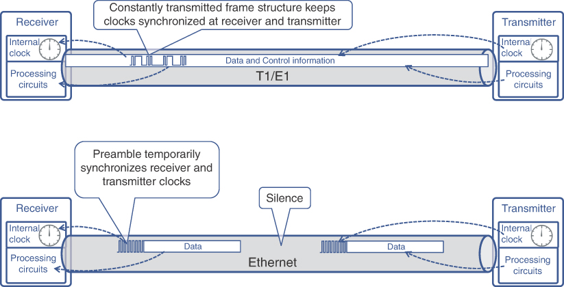
FIGURE 9-1 Synchronizing Transmitter and Receiver on a Transmission Medium
Synchronization, therefore, is a key component of any communication network, and a mobile communication network (MCN) is no exception. In an MCN, in addition to the underlying transport network equipment synchronizing its interfaces for successful transmission of raw data, components of the RAN domain require additional synchronization for RF functions. The remote radio unit (RRU), responsible for RF signal generation, relies heavily on continuous instructions from the baseband unit (BBU), or the distributed unit (DU) in a decomposed RAN architecture, as to when and how to transmit RF signals. In a typical D-RAN environment the collocated RRU and BBU communicate using the Common Public Radio Interface (CPRI) that carries the synchronization information—in addition to the control and user data. However, in a 5G decomposed RAN deployment, the BBU, or rather the DU, may be geographically separated from the RU, relying on the fronthaul network to provide connectivity. This fronthaul network maybe a CPRI Fronthaul (that is, WDM-based Fronthaul carrying CPRI over fiber) or Packetized Fronthaul (that is, carrying RoE or eCPRI). The nature of packetized fronthaul networks is radically different from the constant bitrate (CBR) nature of the CPRI in a D-RAN environment. Such fronthaul traffic might experience unpredictable latency and jitter; hence, the RU and DU cannot rely on the embedded synchronization information in packetized CPRI traffic for synchronizing their clocks. To remedy this, the packetized fronthaul network must provide timing and synchronization to the RU and DU to ensure continued mobile network operation.
The rest of this chapter will focus on the various aspects of synchronization, including the type of synchronization as well as its application and propagation in 5G networks.
Types of Synchronization
Considering time and synchronization as a singular monolithic entity is a common misconception. A closer look at transport networks paints a more intricate picture of the various aspects that need to be coordinated. The synchronization of transport network equipment is made up of more than just the time of day (ToD), which is probably the only interpretation of time in everyday life. The ToD refers to an exact moment in the regular 24-hour daily cycle and is aligned with the planetary time, maintained at both the global and individual government levels through the use of highly accurate atomic clocks. The concept of planetary time and atomic clocks is covered later in this chapter. Synchronizing the ToD across devices in a given network is an important aspect of ongoing operations. If all the devices in the network are aware of the ToD, event logging with timestamping can be used to correlate and troubleshoot problems in the network.
Nevertheless, in addition to the ToD, mobile communication networks also require frequency and phase synchronization. For someone new to timing and synchronization topics, the concepts of frequency and phase might be hard to grasp, and, as such, this section will try to use everyday examples to convey these concepts before delving deeper into frequency, phase, and time of day synchronization in mobile networks.
To understand these concepts, consider the example of two identical, fully operational clocks. As these clocks are identical, it can be safely assumed that both clocks will be ticking every second at the same speed; hence, these clocks are considered to be in frequency sync with each other. However, if these clocks do not tick at the exact same moment, they will not be considered phase synchronized or phase aligned. If one of the clocks starts running faster or slower due to an internal error or external parameters, its perspective of what constitutes 1 second will change. In other words, the frequency at which this clock ticks will change. Should this happen, the frequency synchronization between the two clocks will be lost, and their phases cannot be aligned either. Sure enough, on a linear timescale, and assuming both clocks stay operational, it is possible that the two clocks may start their second at the exact same moment, thus providing a singular, momentary instance of accidental phase alignment. However, because they now operate on separate frequencies, this phase alignment will be a one-off, accidental event with no meaningful significance.
The public transportation system could be another example that showcases the extent to which frequency and phase are interrelated. The schedules of buses and trains in modern public transport systems are carefully synchronized to provide riders the benefit of switching between the two transport mediums as quickly as possible. Consider the case of a central station that acts as an exchange point between a particular bus and a train route used by a substantial number of riders. If this specific bus and train arrive at the station every 55 minutes and stay there for another 5 minutes, their frequencies are considered to be synchronized. Suppose the bus always arrives 30 minutes past the hour, but the train arrives at the top of every hour; the riders who need to switch between the two will have to wait for an extended period of time. However, if both the train and bus routes are synchronized such that they both arrive at the top of the hour and stay for 5 minutes, this allows the riders to switch between the two without wasting any time. Now, the bus and train routes are not only frequency synchronized (arriving every 55 minutes and staying at the station for 5 minutes), they are also phase synchronized, as they both arrive and leave at the exact same time—that is, at the top of the hour. Thus, by aligning both frequency and phase, the public transportation network introduces efficiency in its system.
The 5-minute wait time between the bus or train arriving and departing also serves as a buffer should their arrival frequencies get temporarily out of sync, thus impacting their phase alignment as well. It could be a result of additional traffic on the road, unexpected road closures forcing the bus to take longer routes, or simply encountering too many traffic lights, resulting in the bus getting delayed and potentially losing its alignment and synchronization with the train. If these factors result in a cumulative delay of less than 5 minutes, there is still a possibility that riders will be able to switch between the bus and train in a timely fashion. Hence, the 5 minutes constitute the total time error budget (that is, either the bus or the train could be misaligned with each other for up to a maximum of 5 minutes without a major impact). Should the delays exceed 5 minutes, the system suffers performance degradation. In other words, the time error budget is the maximum inaccuracy a system can handle, before the time errors start impacting the overall operation of the system.
In short, frequency refers to a cyclical event at a predetermined interval, and frequency synchronization between two or more entities ensures that all entities perform the desired function at the same intervals. Examples of frequency synchronization in a mobile communication network include the internal oscillators of the RAN equipment (such as the RRU) oscillating at a predetermined interval, thus generating a predetermined frequency. On the other hand, phase refers to an event starting at a precise time, and phase alignment or phase synchronization refers to multiple frequency aligned entities starting the said event at precisely the same moment in time. An example of phase alignment in mobile communication networks can be a TDD-based system where the base station and mobile handsets must be in agreement on when a timeslot starts. Figure 9-2 outlines the concepts of frequency and phase synchronization.

FIGURE 9-2 Frequency and Phase Synchronization
Similar to how the 5-minute wait time acts as a measure of time error budget in the train and bus example, frequency, phase, and ToD have their own measure of time error budgets as well. The time error for ToD is perhaps the easiest to understand and envision. A second is universally considered to be the standard measure of time, as it refers to an exact moment in the 24-hour daily cycle. A ToD synchronization error is usually measured in seconds or milliseconds. The unit of measure for phase synchronization errors is similar to ToD in terms of base unit but differs significantly in terms of granularity. Whereas the ToD is measured in seconds or milliseconds, phase synchronization and its errors are measured in sub-microseconds or nanoseconds. The unit of measure for frequency sync errors is parts per million (ppm) or parts per billion (ppb). Here, parts refers to an individual frequency cycle, and ppm or ppb refers to an inaccuracy in a frequency cycle over the stated range. For instance, 10 ppm refers to an allowance of gaining or losing 10 cycles every 1 million iterations. Likewise, a 10 ppb allowance is the equivalent of gaining or losing 10 cycles every 1 billion iterations.
Why Synchronization Is Important in 5G
Undoubtedly, modern radio communication systems provide the convenience of being connected to the network without rigid constraints of tethering wires. Radio waves easily propagate in every direction and can cover large areas. However, the flip side of this is the interference of signals from multiple transmitters, making it hard and sometimes impossible to receive a transmission reliably without taking special measures. Chapter 1, “A Peek at the Past,” and Chapter 2, “Anatomy of Mobile Communication Networks,” briefly introduced the phenomenon of interference, along with various approaches to manage it in earlier mobile communication networks. The easiest of these was to use different frequencies in neighboring cells, thus greatly reducing the potential for signal interference. Unfortunately, this approach is unsustainable, as the usable frequency ranges for MCN are quite narrow. Rapidly increasing demand for bandwidth pushed later generations of mobile communication networks to use more sophisticated ways to share the transmission media (that is, radio waves).
As explained in Chapter 3, “Mobile Networks Today,” and Chapter 5, “5G Fundamentals,” LTE and 5G NR use Orthogonal Frequency-Division Multiple Access (OFDMA) with its 15KHz subcarriers. The use of narrow subcarriers imposes strict requirements on the frequency accuracy used in both base station radios and mobile devices. High frequency accuracy is crucial for keeping adjacent subcarriers free from interference. The 3GPP specification requires 5G NR frequency accuracy on the air interface to be in the range of ±0.1 ppm for local area and medium-range base stations and ±0.05 ppm for wide area base stations.1
Modern electronic equipment uses high-quality crystal oscillators to generate stable frequencies; however, crystal oscillators are susceptible to the fluctuations of environmental parameters such as temperature, pressure, and humidity as well as other factors such as power voltage instabilities. Although it does not completely eliminate the frequency drift, the use of specialized temperature-compensated crystal oscillators (TCXO) in the radio and processing equipment of the MCN reduces the effects of these fluctuations. Combined with an externally provided, highly stable reference frequency signal, the required frequency accuracy can be achieved at the base station. The accuracy of the reference frequency signal provided by the network should be substantially better than the required 50 ppb (±0.05 ppm in 3GPP documents) for the LTE and 5G networks, as explained in the ITU-T G.8261/Y.1361 recommendation, and many documents suggest the frequency reference provided by the network should have an accuracy of better than 16 ppb.2 A similar approach is used in the mobile device, where the carrier frequency generation circuit is corrected using the frequency extracted from the base station’s signal for higher accuracy. Frequency division duplex–based (FDD-based) mobile systems, as discussed in Chapter 2, require frequency synchronization for continued operations.
Phase synchronization, or rather time alignment, is another crucial signal transmission parameter in MCN. The term phase synchronization might be confusing for architects not very familiar with the synchronization aspect of mobile networks. The concept of phase here is used to describe the start of a radio frame. In TDD-based transmission systems, where both the base station and mobile device use the same frequency for upstream and downstream transmissions, the alignment of timeslots between the two is critical, and therefore phase synchronization is essential.
Additionally, when two neighboring cells use the same frequency bands, it is crucial to coordinate the usage of OFDM resource blocks between these cells. Coordination between the cells ensures that overlapping OFDM resource blocks are not used to transmit data for the subscribers at the edges of the cells, where interference can cause transmission errors. In simple terms, the neighboring cells coordinate which resource blocks are used and which are left for the other cell to use. In a perfectly aligned transmission between the cells, the resource block used by one cell is matched by the void or unused blocks by the other. This allows the sharing of resource blocks between the two receivers residing in the proximity of the cell edge. If the phase alignment is not achieved between the neighboring cells, the resource blocks used in both cells start overlapping, causing transmission errors, as shown in Figure 9-3.

FIGURE 9-3 Intercell Interference and Synchronization
The required precision of time alignment between multiple neighboring cells is dependent on functionality implemented at the cell sites. 5G NR allows intercell time deviation of ±1.5μs with ±1μs budget allowed for network transport. This budget also allows the use of coordinated multipoint (CoMP) transmission. However, advanced antenna features impose even more demanding requirements. For instance, carrier aggregation in 5G NR imposes the tight 260ns maximum absolute error for intra-band allocations. The time alignment tolerance for multi-radio MIMO transmission is even tighter, with a whooping 65ns maximum error.3
Collectively, these strict requirements imposed by advanced radio functions, scalable spectrum utilization, and reliable connectivity make it even more important for ToD, frequency, and phase in a 5G deployment to be highly synchronized. This is achieved by ensuring that highly reliable and uniform clock sources are used to acquire timing information across the 5G network, and when that’s not possible or feasible, then the MCN is able to accurately carry this timing information across. The next two sections discuss these topics in further detail.
Synchronization Sources and Clock Types
Broadly speaking, a clock is a device that counts cycles of a periodic event. Of course, such a clock does not necessarily keep time in seconds or minutes but rather in measures of periodic event cycles. By selecting the appropriate periodic event and denominator for the cycle count, a clock can produce meaningful timing signals for the desired application. Similar to how mechanical clocks use pendulums or weights attached to a spring, commonly referred to as oscillators, electronic equipment relies on circuits generating a periodic change in voltage or current. Although a rudimentary oscillator circuit made of resistors, capacitors, and inductors can do the job of generating the desired frequency, it lacks the accuracy to qualify as a useful reference. Clearly, the accuracy of an oscillator depends on its components’ precision. Nevertheless, it is usually not feasible to increase the precision of a simple oscillator’s components as another, more practical approach became popular in the electronics industry in the previous century.
By far the most popular way to build a simple yet accurate electronic clock is to use quartz crystal oscillators in its frequency-generating circuit. Voltage applied to the tiny slice of quartz in such an oscillator creates mechanical stress. When this voltage is removed, the dissipating stress creates electricity. This process would then repeat at the resonant frequency of this quartz slice until all initial energy is dissipated in the form of heat. However, if the signal is amplified and applied back to the crystal, a stable constant frequency can be produced. The resonant frequency of a quartz crystal oscillator depends on the shape and size of the slice of quartz, and it can easily be manufactured today with great precision. For example, virtually every electronic wristwatch today uses a quartz crystal oscillator manufactured with the resonance of 32,768Hz. The sine wave cycles are then counted, and the circuit provides a pulse every 32,768 cycles, precisely at each 1 second interval—that is, a 1 pulse-per-second (1PPS) signal. The accuracy of clocks using quartz crystal oscillators is typically in the range of 10 to 100 ppm, which equates to roughly 1 to 10 seconds per day. This time drift may be acceptable for common wristwatch use but may be catastrophic for automated processes and other applications that rely on much more accurate timekeeping.
Besides the manufacturing precision, other factors affect the accuracy of a quartz crystal oscillator. Temperature fluctuations and power voltage fluctuations are among the usual suspects. Luckily, these factors can be compensated for, and more sophisticated temperature-compensated crystal oscillator (TCXO) and oven-controlled crystal oscillator (OCXO) can provide substantially more accurate frequency sources. The accuracy of an OCXO can be as good as 1 ppb, which translates to a drift of roughly 1 second in 30 years.
For clock designs with even higher accuracy, a different physical phenomenon is used as the source of a periodic signal. Although the underlying physics of this phenomenon is quite complex, suffice it to say that all atoms transition between internal states of a so-called hyperfine structure (that is, energy levels split due to the composition of an atom itself). These transitions have very specific resonant frequencies, which are known and can be measured with great precision. Because the atoms’ resonant frequencies are used in lieu of oscillators, a clock using this phenomenon is generally called an atomic clock. The resonant frequency of cesium atoms used in atomic clocks is 9192631770 Hz.4 The measured resonant frequency is not used directly by the atomic clock but rather to discipline quartz oscillators, which are still used to generate the actual frequency for the clock’s counting circuits. Cesium atomic clocks are some of the most accurate clocks and can maintain an accuracy of better than 1 second over 100 million years. The International Bureau of Weights and Measures relies on the combined output of more than 400 cesium atomic clocks spread across the globe to maintain accurate time. This is considered the ultimate planetary clock and is referred to as Coordinated Universal Time, or UTC.5
Cesium atomic clocks are ultra-accurate, but they have bulky designs and high costs. For many practical applications, the accuracy of cesium clocks is not needed, and rubidium atomic clocks can commonly be used instead of cesium-based devices. Rubidium atoms are used to build much more compact and cheaper atomic clocks; however, their precision is lower than that of a cesium clock by a few orders of magnitude. Rubidium atomic clocks have an accuracy sufficient for most practical purposes and can maintain time accuracy within 1 second over 30,000 years. Due to their portability, rubidium clocks are commonly used as reference clocks in the telecom industry, military applications, and in the satellites of many countries’ global navigation satellite systems (GNSSs).
GNSSs are well known for the great convenience they provide in everyday navigation. Aircrafts, ships, cars, and even pedestrians routinely use navigation apps on their computers and mobile devices. These apps calculate the current position of a user based on the difference of timing signals received from multiple GNSS satellites. A few countries and unions have developed and launched their own version of GNSS, such as the United States’ Global Positioning System (GPS), the European Union’s Galileo, Russia’s Global Navigation Satellite System (GLONASS), and China’s BeiDou. Although Japan’s Quasi-Zenith Satellite System (QZSS) and the Indian Regional Navigation Satellite System (IRNSS) are also systems designed for satellite navigation and provide accurate time, they are regional systems designed to augment the GPS system for their respective regions.
Although navigation can be perceived as the main purpose of any global navigation satellite systems, these systems are also used to provide accurate time reference (called timer transfer) for many applications, including mobile communication networks. The GNSS signals encode both frequency and phase as well as ToD information, along with the information about each satellite’s orbit. In fact, the major goal of all GNSS satellites is to maintain accurate time and transmit it to the consumers on Earth’s surface and in the air. Satellite transmissions can cover large areas effectively and are ideal for the distribution of a reference timing signal.
As mentioned earlier, due to their good accuracy and portability, GNSS satellites use rubidium clocks. Satellites’ clocks are also periodically synchronized with each other as well as with the terrestrial atomic clock sources to maintain the highest accuracy of the time signals necessary for navigation calculations and providing a timing reference to surface receivers, as shown in Figure 9-4.

FIGURE 9-4 Synchronization in GNSS
Interestingly enough, due to Earth’s gravity, the clock on a satellite runs a notch faster compared to the same clock on the ground. The navigation apps routinely calculate necessary corrections to account for this phenomenon, called gravitation time dilation and explained by Einstein’s theory of General Relativity.
Normally, GNSSs provide timing signals with very high accuracy. For example, more than 95% of the time, the time transfer function of a GPS system has a time error of less than 30 nanoseconds.6 Additional errors could be introduced by the processing circuit of a GNSS receiver, and most GPS clock receivers used in the telecom industry can provide time reference with an error of less than 100 nanoseconds to the time reference signal consumers.
Implementing Timing in Mobile Networks
So far, this chapter has discussed various concepts about time, its synchronization, and its importance in 5G transport networks. As mentioned earlier, network timing is not a monolith but rather is composed of frequency, phase, and time of day—all of which have to work in unison to provide timing and synchronization for various scenarios. Generally speaking, basic FDD-based mobile networks require only frequency synchronization, whereas TDD-based mobile networks require strict phase synchronization. However, most multi-radio transmissions and intercell interference coordination (ICIC) scenarios—whether FDD or TDD based—also require strict phase synchronization.7 As previously mentioned, phase and frequency are interrelated; hence, it is always considered a best practice to implement both phase and frequency synchronization in mobile networks. ToD is important for all networks due to its use for correlating events and failures using logs with accurate timestamps.
In a traditional D-RAN implementation, the CPRI between the co-located RU and BBU is responsible for carrying the synchronization information. The RU has to be in constant sync with the BBU since the DU component of the BBU provides the necessary instructions to the RU to perform RF functions. In this case, the synchronization traffic usually remains confined to the cell site location; however, the instructions provided by the DU components of the BBU often require synchronization with neighboring cell sites’ BBUs for use cases such as ICIC implementations. If all the cell sites directly acquire their timing signal from a highly reliable, common, and accurate source such as atomic clocks in the GNSS-based satellites, the BBUs will be considered in sync with each other and thus the mobile transport network will not be explicitly required to distribute timing and synchronization information. In this case, the satellite-based timing signal is acquired directly at the BBUs using a GNSS antenna, and any required timing information is provided to the RU through the CPRI. There is no need to acquire or distribute the timing signal to the CSR, thus removing any dependencies with respect to the timing interfaces or protocols supported on the CSR. This is the exact deployment model for a large number of existing mobile deployments today and is shown in Figure 9-5.

FIGURE 9-5 D-RAN Cell Sites Synchronization via GNSS
In cases where GNSS signals might not be acquired at every cell site, the mobile backhaul would need to distribute a synchronization reference across the cell sites. One of the primary reasons for such a scenario could be security concerns, stemming from the fact that different GNSSs are controlled by individual governments. For instance, the Galileo-based GNSSs became operational in 2016, and prior to that, if a Europe-based service provider wanted to avoid using GPS, GLONASS, or BeiDou satellites, it would have to implement terrestrial timing signal acquisition and transport mechanisms.8 Additionally, with the gradual move toward a decomposed RAN architecture comprising sometimes geographically distanced RUs and DUs, the fronthaul now has to always transport timing information between the cell site and far-edge DCs, even though the rest of the mobile transport may not have to be aware of, or even carry, the timing information. Hence, it can be concluded that while distributing timing and sync information using transport networks was optional in the pre-5G networks, it is absolutely mandatory for a 5G transport network to implement the capabilities of distributing timing and synchronization information to cell sites, as demonstrated in Figure 9-6.

FIGURE 9-6 Distributing Time Through Fronthaul Network
The packetized fronthaul network relies on packet-based transport protocols that are asynchronous in nature (for example, Ethernet), which cannot be used as is to distribute timing information. In order to reliably transport timing information across this packetized fronthaul, additional mechanisms are required to distribute frequency, phase, and ToD information. These mechanisms are Synchronous Ethernet (SyncE) for frequency synchronization and accuracy, Precision Time Protocol (PTP) for phase alignment, and Network Time Protocol (NTP) for ToD synchronization.
The rest of this chapter will cover how the reference timing signal is acquired, packetized, and propagated through the mobile transport networks.
Acquiring and Propagating Timing in the Mobile Transport Network
Over the past several years, the use of GNSS has emerged as an effective and cheap mechanism to distribute the reference timing signal in mobile communication networks. Using an antenna, the network device(s) would acquire the satellite signal from one of the GNSS constellations—GPS, Galileo, GLONASS, or BeiDou. This device can be a router or other specialized clocking devices from a vendor that specializes in timing and clocking devices, such as Microsemi.9 The GNSS-based timing signal is a single composite signal that carries ToD, frequency, and phase information from the atomic clock aboard the GNSS satellites in Earth’s orbit. The network device receiving the GNSS is considered a primary reference clock (PRC) if it acquires only the frequency signal or a primary reference timing clock (PRTC) if it acquires the frequency, phase, and ToD signal. The PRTC then distributes the phase, frequency, and ToD reference to the rest of the packet network using PTP, SyncE, and NTP.
The GNSS antenna requires a clear, unobstructed view of the sky, which in some cases limits the places where a GNSS signal can be acquired in mobile transport networks. It might be beneficial to acquire the GNSS signal at a more central location such as a far-edge or edge DC and propagate it down to the cell sites. However, in a lot of cases, the mobile service provider does not own the far-edge or edge DC and, as part of its lease agreements, might not have access to the roof for GNSS antenna installation. In these cases, the GNSS antenna could be installed at the cell sites and the timing signal distributed to the rest of the mobile network. Acquiring GNSS at multiple cell site locations also allows for timing signal redundancy; that is, in the case of a GNSS reception problem on one site, another site could take over and be used as the reference clocks.
While very common and easy to use, GNSS signals are susceptible to jamming as well as spoofing. Technological advances have made devices that can jam GNSS easily accessible. While an individual with malicious intent can access GNSS jammers and jam signals within a few kilometers, disrupting mobile services in the process, the major concern for national governments is the use of jamming technologies by foreign governments or their proxies. Given the importance of satellite-based navigation and timing systems, most governments treat GNSS jamming as a threat to their national security and are taking actions to safeguard the system. For instance, the U.S. Department of Homeland Security (DHS) considers GPS (the U.S. version of GNSS) a “single point of failure for critical infrastructure.”11 Recognizing the importance of an alternate to GPS, the U.S. Congress passed a bill called National Timing Resilience and Security Act of 2018 in December of 2018 aimed at creating a terrestrial-based alternative to GPS in order to solve any problems that may arise from GPS signal jamming. Similar efforts are underway in other geographies as well.
In mobile communication networks, the service providers sometimes use anti-jamming equipment at their GNSS receivers in order to mitigate efforts to jam the GPS signal. Another approach is the use of a terrestrial frequency clock to provide a reliable source of frequency sync in case of a GNSS failure. If phase is fully aligned throughout the network, an accurate frequency signal can keep phase in sync for an extended period of time in case of a GNSS failure.
Most modern cell site routers are equipped with a specialized interface that can be connected to a GNSS antenna, acquire the signal, and propagate it to the rest of the network. Depending on the vendor implementation, the routers might also have the input interfaces to acquire the reference signal for phase, frequency, and ToD individually. Acquiring each timing component individually typically requires a specialized device at the premises that can act as the PRC or PRTC and provide individual frequency, phase, and ToD references to the router. The reference signal for frequency is acquired through a 10MHz input interface, which can be connected to a frequency source that provides a highly accurate 10MHz frequency for the networking device to align its internal clock to. Older systems used a Building Integrated Timing Supply (BITS) interface for frequency acquisition, but today BITS is seldom if ever used. Phase alignment is achieved by using a 1PPS (sometimes also called PPS) interface. As the name suggests, the 1PPS interface provides a sharp pulse that marks the start of a second and thus allows the router (or other device) to align its phase to the start edge of the pulse. The duration of this pulse is slightly less than 1 second, and the start of the second is marked by the start of the pulse.
Most networking equipment has the capability for both these options. Figure 9-7 shows the front panel of Cisco and Juniper routers with interfaces for both GNSS signal and individual frequency, phase, and ToD alignment.12, 13

FIGURE 9-7 Front Panels of Cisco and Juniper Routers with Timing Acquisition Interfaces
Once the timing signal is acquired, it needs to be propagated throughout the rest of the network to distribute the frequency, phase, and ToD information. The rest of this section will discuss the various protocols and design models used to efficiently and accurately distribute timing information through the mobile transport network.
Synchronous Ethernet (SyncE)
The proliferation of Ethernet beyond its original application area of local area networks (LANs) into the territory of traditional long-haul SONET/SDH transport helped keep the cost of higher-speed wide area network (WAN) interfaces in check. Although circuit-emulation services over packet-based networks allowed for connecting islands of traditional TDM networks over Ethernet, synchronization between the two sides of an emulated circuit required additional considerations. ITU-T defined an architecture and procedures, known as Synchronous Ethernet (SyncE), to propagate a synchronization signal over a packet-based network. The synchronization model of SyncE is designed to be compatible with that of SONET/SDH and, by design, can only provide frequency synchronization and information about the clock quality. The following few ITU-T standards define SyncE architecture and operation:
G.8261: Timing and synchronization aspects in packet networks
G.8262: Timing characteristics of a synchronous equipment slave clock
G.8264: Distribution of timing information through packet networks
As mentioned earlier, the Ethernet interface synchronizes its receiver to the bitstream on the wire only for the duration of a frame sent by the remote node. In fact, this temporary synchronization can be used for frequency propagation between SyncE-capable devices. For such a synchronization propagation method to be effective, a SyncE-capable device should have a good oscillator to keep the frequency generator of its clock from drifting when synchronization from a better clock is not available. When such a condition happens, where a device loses its reference signal, the device is said to be operating in holdover mode.
Clock accuracy used in a typical Ethernet device is quite low (around ±100 ppm). SyncE-capable devices require clocks with ±4.6 ppm accuracy or better, as per the G.8261 standard.14 Additionally, the clock on SyncE-capable devices can be locked to an external signal.
The frequency generator of a SyncE-capable device can be locked to a frequency signal extracted by the specialized Ethernet physical layer circuit from the bitstream received on the interface. Sync-E-capable devices constantly send a reference signal on the Ethernet interface. This signal does not interfere with actual packet transmission but is incorporated into it. The edges of the signal on the wire, or in the optical fiber, are used as a reference for the SyncE-capable device’s frequency generator. The internal clock is then used to synchronize all signal edges of the transmitted Ethernet frames, thereby providing a frequency reference for downstream SyncE-capable devices.
In SyncE applications, the source of a highly accurate frequency signal such as an atomic clock is referred to as a primary reference clock (PRC). When the internal clock of a SyncE-capable device is locked to a PRC via a timing acquisition interface, it becomes the source of frequency synchronization for other SyncE-capable devices. The frequency synchronization is propagated hop by hop through the SyncE-enabled network from the PRC-connected SyncE-capable devices to the downstream devices and eventually to the ultimate consumers of frequency synchronization. Figure 9-8 shows the mechanism of frequency (clocking) recovery from the signal edges of an Ethernet frame and sourcing of the frequency synchronization for the downstream hop-by-hop propagation.

FIGURE 9-8 Frequency Synchronization with SyncE
SyncE-capable devices can be explicitly configured with the synchronization hierarchy or can automatically identify it based on the exchange of messages in the Ethernet Synchronization Messaging Channel (ESMC) defined by ITU-T G.8264.15 This messaging channel is created by exchanging frames with EtherType set to 0x8809 and is required for compatibility with SONET/SDH synchronization models. ESMC channels carry a Quality Level (QL) indicator for the clock, which is in essence a value representing the clock position in the hierarchy (that is, how far the clock is from the PRC and the operational status of the clock). QL values are exchanged between SyncE-enabled devices and used to identify upstream and downstream ports in the synchronization hierarchy.
Although it requires hardware enhancements, SyncE architecture is very effective in propagating frequency synchronization, but it cannot propagate phase or ToD information. While NTP continued to be used for ToD propagation, Precision Time Protocol (PTP) was defined to transport phase synchronization information in modern networks supporting mobile communication and other applications.
Precision Time Protocol
Communication networks have used Network Time Protocol (NTP, discussed later in this section) since the 1980s to distribute timing information (more specifically the ToD). Its accuracy, or rather the lack thereof, however, left a lot to be desired for most modern applications. These applications, such as mobile communications, require much stricter accuracy (typically, to the tune of sub-microseconds), whereas NTP provides accuracy in the magnitude of multiple milliseconds at best.16
As discussed earlier, one of the ways to provide accurate timing information to relevant devices is the use of GNSS on all devices, thus acquiring a common reference time from a satellite-based atomic clock. However, it might not always be feasible, or even possible, to set up a GNSS antenna next to every device that needs phase alignment. Common reasons for not being able to implement GNSS everywhere could be excessive cost, lack of a suitable location for antenna placement, unfavorable locations, and national security concerns, among others. In short, the existing timing transport protocol fell short of the required features, and the only viable alternative of providing an atomic clock input everywhere was not realistic.
Precision Time Protocol (PTP), often called IEEE 1588 PTP after the IEEE specification that defines the protocol, fills this gap by not only providing sub-microsecond accuracy but also the convenience and cost-effectiveness of acquiring the timing reference at a few select locations and distributing it through the packet network. The first implementation of PTP, called PTPv1, was based on the IEEE 1588-2002 specification, where 2002 refers to the year the specification was published. The specification was revised in 2008 and again in 2019 to provide enhancements such as improved accuracy and precision. The implementation of IEEE 1588-2008 is called PTPv2, whereas IEEE 1588-2019 is referred to as PTP v2.1.
PTP Operation Overview
From PTP’s perspective, any device participating in timing distribution is considered a clock. This includes not only the atomic clock that generates the reference timing signal but all the routers in the transport network that process PTP packets as well. A PTP-based timing distribution network employs a multi-level master-slave clock hierarchy, where each clock may be a slave for its upstream master clock and simultaneously act as a master to its downstream clock(s). The interface on the master clock, toward a slave clock, is referred to as a master port. Correspondingly, the interface on the slave clock toward the master is called a slave port. The master port is responsible for providing timing information to its corresponding slave port. These are not physical ports but rather logical PTP constructs that provide their intended functions using a physical interface. In most cases, the master and slave PTP functions reside on directly connected devices. This is, however, not the only mode of PTP operations, as covered in the PTP deployment profiles later in this chapter.
Note
Use of the terms master and slave is only in association with the official terminology used in industry specifications and standards and in no way diminishes Pearson’s commitment to promoting diversity, equity, and inclusion and challenging, countering, and/or combating bias and stereotyping in the global population of the learners we serve.
PTP uses two-way communication to exchange a series of messages between the master and slave ports. These messages can be broadly classified in two categories: event messages and general messages. An event message carries actual timing information and should be treated as priority data due to its time-sensitive nature. By contrast, a general message carries non-real-time information to support various PTP operations. An example of a general message is the announce message, which, as the name suggests, announces the capability and quality of the clock source. For instance, a master port may send periodic announce messages to its corresponding slave port that contain information such as clock accuracy and the number of hops it is away from the clock source, among other information. The announce messages are used to select the best master clock based on the PRTC and build a master-slave hierarchy through the network using the Best Master Clock Algorithm (BMCA) defined by IEEE 1588. Here are some of the other relevant PTP messages that help distribute time through the network:
Sync: An event message from the master port to slave port, informing it of the master time. The sync message is timestamped at the egress master port.
Follow_Up: An optional event message that carries the timestamp for the sync message if the original sync message is not timestamped at egress.
Delay_Req: A message from the slave port to master port to calculate the transit time between the master and slave ports.
Delay_Resp: The master port’s response to delay_req, informing the slave port of the time delay_req was received.
Figure 9-9 shows a basic event messages exchange between master and slave ports to distribute timing information. The sync message is initiated by the master port with egress timestamp either included or carried in the follow_up message, depending on the vendor implementation. Accurate timestamping of a sync message at the last possible instant as the message is leaving the master clock is critical for time calculation. However, recording the exact time the message leaves the interface and stamping it on the outgoing packet simultaneously may present technical challenges. To alleviate this, PTP specifications allow a two-step process, where the timestamp is recorded locally at the master when the sync message is transmitted but is sent to the slave in a subsequent follow_up message. When the sync message (or the follow_up message) is received at the slave port, the slave clock becomes aware of not only the reference time at the master but also the time at which the sync message is sent (called t1) and the time at which the sync is received (called t2). However, t1 is marked relative to the master’s internal clock, while t2 is marked relative to the slave’s internal clock, which may have drifted away from the master. Thus, if the slave wants to synchronize its internal clock, it must be aware of the transit time between the two. This is accomplished by the slave sending a delay_req message to the master, which then responds with a delay_res message. The timestamp on the delay_req transmission is called t3, whereas t4 is the time when the delay_req is received at the master. The master clock notifies the slave of the receive time (that is, t4, using the delay_res message).

FIGURE 9-9 PTP Sync and Delay Messages Between Master and Slave Ports
In order to achieve time synchronization with its master, the slave clock must calculate how much its internal clock has drifted from the master—a value defined as offsetFromMaster by IEEE 1588. Once this offsetFromMaster value is calculated, the slave clock uses it to adjust its internal clock and achieve synchronization with the master clock. The offsetFromMaster is calculated using the two data sets known by the slave clock: t2 and t1, and t3 and t4. In an ideal scenario, with a transmission delay of 0 between the master and slave clocks, the values t1 and t2 should be identical, even though they are timestamped using the master and slave clocks, respectively. In this scenario, any deviation between the two timestamps could only mean that the two clocks are not synchronized; whatever the difference is between the two timestamps should be added (if t1 > t2) or removed (if t2 > t1) from the slave clock. However, every real-world scenario incurs some transit time, however miniscule, between the master and slave clocks. Using the meanPathDelay, which could only be calculated by averaging the timestamp difference for transit time in both directions, gives a fairly accurate picture of the actual offset between the master and slave clocks. IEEE 1588 specifications define the logic and process of calculating this offset in greater detail, but it eventually comes down to the following equation:17
offsetFromMaster = (t2 − t1 + t3 − t4) / 2
Figure 9-10 outlines three scenarios and their respective calculations for measuring the offsetFromMaster. The first scenario assumes the master and slave clocks are in perfect synchronization and thus the offsetFromMaster is 0. The other two scenarios assume that the slave clock is either ahead of or lagging behind the master clock by a value of 1μsec. Although the transit time stays constant at 2μsec in all scenarios, the timestamping in scenarios 2 and 3 is impacted by this inaccuracy. However, in each of these three scenarios, the preceding equation calculates the offsetFromMaster correctly. Once calculated, the offsetFromMaster is used to adjust the slave clock and maintain its synchronization with the upstream master clock, as also shown in the figure.

FIGURE 9-10 Calculating offsetFromMaster for Phase Synchronization Using PTP
As seen in all the example scenarios in Figure 9-10, PTP relies heavily on the assumption that the forward and reverse paths between master and slave clocks are symmetrical. In timing distribution networks, this property of equal path in either direction is referred to as path symmetry. However, if there is any path asymmetry between the master and slave clocks (that is, the transit time from master to slave and from slave to master differs), the offset calculation will be skewed and will eventually lead to time synchronization errors. Thus, any transit difference due to asymmetry must be taken into account by PTP during the offset calculation. The asymmetry in transit times could result from a few different factors but is usually due to the difference in cable lengths between transmit and receive ports. Just a minor asymmetry in the length of cable in either direction, sometimes introduced simply by leaving a few extra feet of slack in one strand of fiber, could lead to different transit times between the master and slave clocks in either direction. Even with transceivers using a single strand of fiber for transmit and receive, the chromatic dispersion properties of different wavelengths may cause light to travel at different speeds in either direction. This can potentially result in asymmetry of message travel time between master and slave. The actual transit time difference in both directions could be miniscule, but for a protocol like PTP, where accuracy requirements are in the sub-microseconds, even a small and otherwise negligible discrepancy in transit time between the master and slave clocks could negatively impact PTP accuracy. To remedy any possible problems, path asymmetry must be measured at the time of network deployment and accounted for as part of PTP configuration. Various test equipment vendors provide specialized tools to measure network asymmetry. As long as the network asymmetry is measured, accounted for, and remains unchanged, PTP will continue to operate correctly and provide time synchronization using the packet network.
PTP Clocks
As mentioned in the previous section, any network device participating in PTP operation is considered a clock. It is already mentioned in the previous section that the GNSS-based atomic clock provides the reference timing signal to a PRTC. From PTP’s perspective, the PRTC that provides reference time to the packet networks is called a grandmaster. Sometimes the terms grandmaster and PRTC are used interchangeably, as the two functions are often embedded on the same device in the network. However, there is a clear distinction between the two. A PRTC refers to the source for frequency, phase, and ToD, whereas a grandmaster is a PTP function where packetized timing information is originated.
For distributing timing information from the PRTC to the rest of the devices in a packetized timing distribution network, IEEE 1588 defines various types of network clocks:
Ordinary clock (OC)
Boundary clock (BC)
Transparent clock (TC)
An ordinary clock, or OC, is a device that has only one PTP-speaking interface toward the packet-based timing distribution network. Given that PTP networks are usually linear in nature—that is, PTP messages flow from a source (grandmaster or PRTC) to a destination (a timing consumer)—an OC can only be a source or a destination. In other words, an OC is either a grandmaster that distributes timing reference to the network (that is, an OC grandmaster) or a consumer of the timing information from the network (that is, an endpoint). A boundary clock, or BC, on the other hand, is a device with multiple PTP-speaking ports. A BC is simultaneously a master for its downstream slave clocks and a slave to its upstream master.
A transparent clock, or TC, does not explicitly participate in the PTP process, although it allows PTP messages to transparently pass through it. IEEE 1588 defines two different types of transparent clocks—an end-to-end TC and a peer-to-peer TC—although only the end-to-end TC is used in telecommunications networks.18 An end-to-end TC records the residence time of a PTP message (that is, the time it takes for the packetized PTP message to enter and exit the TC). This information is added to the correctionField in the PTP header of the sync or follow_up message transiting through the TC. The correctionField helps inform the master and slave clocks of any additional time incurred while transiting the TC. This effectively eliminates the transit time introduced while the packet is forwarded through the TC.
Figure 9-11 shows a PTP-based timing distribution network with different types of clock and ports.

FIGURE 9-11 PTP Clock and Port Types in xHaul Network
PTP Deployment, Performance, and Profiles
IEEE has defined the mechanics of the Precision Time Protocol in IEEE 1588 specification with a lot of choices and flexibility for vendor-specific implementations to carry timing information with a very high degree of accuracy. To keep up with the continuously changing landscape, IEEE also revised the specification in the years 2008 and 2019. IEEE, however, by its nature, focuses primarily on research and development as well as the inner details of the protocol itself rather than an end-to-end architecture. Deploying a timing distribution network using PTP, on the other hand, requires a high degree of planning and use of an appropriate network architecture to meet various constraints such as interoperability with older deployments and performance of various types of PTP clocks.
The International Telecommunication Union Telecommunication Standardization Sector (ITU-T) fills that much-needed gap through a series specification and profile definitions aimed at standardizing various aspects of a packet-based timing distribution network. This helps in creating a more cohesive end-to-end deployment model from a network timing perspective, and it also provides a set of expectations for devices participating in the timing processing and distribution. While many different standards are defined by ITU-T for packetized timing networks, this section focuses on the following critical aspects of design and deployment of 5G-ready mobile transport networks:
Reference points in a time and phase synchronization network (ITU-T G.8271)
Performance characteristics of various PTP clocks (ITU-T G.8272 and G.8273)
Deployment profiles for packet-based time and phase distribution (ITU-T G.8265 and G.8275)
ITU-T specifications use a different set of terminologies than what is defined by IEEE 1588 PTP for various clock types. The PTP grandmaster (GM) is called a Telecom Grandmaster (T-GM) in ITU-T terminology and has the same purpose as a PTP GM. However, a T-GM allows more than one master port, whereas a PTP GM was considered an ordinary clock (OC) with a single PTP-speaking port. Similarly, a PTP boundary clock (BC) is called Telecom Boundary Clock (T-BC), a PTP transparent clock (TC) is called a Telecom Transparent Clock (T-TC), and an ordinary slave clock is called a Telecom Timing Slave Clock (T-TSC) in ITU-T terminology. From a mobile xHaul perspective, an RU or a DU could be considered a T-TSC as also shown in the O-RAN Alliance’s Synchronization Architecture and Solution Specification.19 From here on, this chapter will primarily use the ITU-T defined clock terminologies because a lot of deployment-related specification, such as O-RAN Alliance’s Synchronization Architecture and Solution Specification, uses the same ITU-T terminology.
Reference Points in a Time and Phase Synchronization Network
Formally titled Time and Phase Synchronization Aspects of Telecommunication Networks, the ITU-T G8271 specification defines various reference points and their characteristics for a packetized timing distribution network. These reference points, referred to as A through E, span the whole network from the time source to its ultimate destination and everything in between. The G.8271 specification uses the concept of time error budget, which is the maximum inaccuracy allowed at various reference points in the timing distribution network.
The G.8271 reference points are defined from the perspective of time distribution, not from the packet network’s perspective. In fact, the G.8271 reference model views the packet network transport as a monolith, a singular black box, where the timing signal enters through the T-GM and exits just as it’s ready to be provided to the end application. Following are the reference points defined by the G.8271 specification and the error budgets allowed within each:
Reference point A: This is the demarcation at the PRTC and T-GM boundary. The total error budget allowed at the PRTC is ±100 nanoseconds (that is, the PRTC can drift up to a maximum of 100 nanoseconds from the global planetary time).
Reference point B: This refers to the demarcation between the T-GM and the rest of the packet network. G.8271 specs do not define a time error budget for T-GM, but since PRTC and T-GM are implemented together in most implementations, vendors and operators consider the ±100ns deviation for both the PRTC and T-GM combined.
Reference point C: The packet network between the T-GM and the last T-TSC before handing over the timing signal to the end application. The total TE budget allowed for the packet network is ±200 nanoseconds, irrespective of the number of T-BCs used.
Reference points D & E: These reference points correspond with the end application in the ITU-T specification. While ITU-T distinguishes between the T-TSC and end application as two separate entities, telecommunication networks oftentimes refer to the end application as a clock. For instance, the O-RAN timing specification refers to the O-RU as a T-TSC. Additionally, reference point D is optional and only used when the end application further provides the clock to another end application, as shown in Figure 9-12.
ITU-T G.8271 also defines maximum time error budgets for various failure scenarios such as PRTC failure and short-term or long-term GNSS service interruptions. In most failure scenarios, the maximum end-to-end time error from the PRTC to the end application, as defined by ITU-T G.8271, should not exceed 1.5μsec, or 1500 nanoseconds. This 1.5μsec value is inclusive of the usual ±200 nanosecond budget for a packet network resulting from T-BC or T-TSC inaccuracies, as well as any errors resulting from path asymmetry and clocks entering holdover state due to GNSS or PRTC failures. The maximum total time error expected at reference point C is 1.1μsec, or 1100 nanoseconds, and includes up to 380 ns of path asymmetry and 250 ns inaccuracy that may be introduced in case of PRTC failure. The maximum time error allowed for the end application is 150 nanoseconds. Figure 9-12 provides a graphical representation of these reference points and their respective time error budget.

FIGURE 9-12 G.8271 Defined Time and Phase Synchronization Reference Points and Error Budgets
Performance Characteristics of Various PTP Clocks
As stated previously, the packetized timing distribution network is made up of ordinary clocks (OCs) and a boundary clock (BC). These clocks implement the PTP functions to distribute timing information, but they inevitably introduce time errors due to the strict timestamping requirements imposed by PTP. As such, the total time error introduced in the packet network is the combination of the total number of clocks used in the topology and the time error introduced by each one. The commutative value of the time error introduced by all the clocks in the packet network cannot exceed ±200 nanoseconds, as specified by ITU-T G.8271 specification and mentioned in the earlier section.
The time error accumulates while PTP propagates timing over the packet network, but it is not a constant value. ITU-T G.2860, aptly named “Definitions and terminology for synchronization in packet networks,” indeed defines a few different types of time errors that a PTP clock may introduce in a PTP-based timing distribution network. Here are some of the noteworthy error types:
Maximum absolute time error (max |TE|): This is the maximum error allowed by a clock. Under normal circumstances, a clock should be well below the max time error and closer to a constant time error (cTE).
Constant time error (cTE): cTE refers to the mean of time error experienced by the clock over time. ITU-T G.8260 defines cTE as an average of the various time-error measurements over a given period of time. A device’s cTE is often considered an indicator of its quality and accuracy.
Dynamic time error (dTE): Similar to how jitter is used to define the variation of latency in packet networks, dTE is a measure of variation in the time error introduced by the clock. A higher dTE value often indicates stability issues in the clock implementation and/or operation.
Since the introduction of PTP in 2002, network equipment manufacturers have been constantly improving their PTP-enabled devices. But the reality is that most of the functions required for PTP—a good quality internal oscillator, capability of real-time recording and timestamping of sync messages, and so on—are hardware-based functions. Any meaningful leap in the quality of PTP handling and accuracy requires updated hardware. At the time of this writing, ITU-T has defined four classifications of PTP-supporting devices based on their accuracy in handling PTP functions. These classifications are Class A, B, C, and D.
Class A represents the first generation of PTP-supported hardware and is the least accurate with higher allowance of time error budgets. Class B represents an upgraded hardware with better performance than Class A hardware, and Class C offers even better PTP performance than Class B. Class D hardware is expected to surpass the capabilities of Class C PTP devices, but it is not yet available for mobile communication networks. Almost all network equipment providers support Class C timing on their mobile networking equipment portfolio.
ITU-T G.8273.2 defines the time error allowance for Class A, B, and C PTP hardware, as seen in Table 9-1. Specification for Class D is still being finalized at the time of this writing.20
TABLE 9-1 Permissible Time Error for Class A, B, C, and D PTP Clocks
T-BC/T-TSC Class | Permissible max|TE| | Permissible cTE Range |
|---|---|---|
Class A | 100 nanoseconds | ±50 nanoseconds |
Class B | 70 nanoseconds | ±20 nanoseconds |
Class C | 30 nanoseconds | ±10 nanoseconds |
Class D | Not yet defined | Not yet defined |
The classification of a PTP device plays an important role in building a packetized timing distribution network. Recall that, as shown in Figure 9-12, ITU G.8271 specification allows a total time error of ±200 nanoseconds for the packet network irrespective of the number of T-BCs used. For example, when using Class A PTP devices, with a cTE of ±50 nanoseconds, the network topology is limited to a maximum of only 4 PTP-aware devices before the time error budget exceeds the ±200 nanosecond threshold. Conversely, using a Class B or Class C device allows a maximum of 10 or 20 devices, respectively.
As the PTP clock classification is hardware dependent, a software-only upgrade will not convert a Class B timing device into Class C. Converting an existing device class (for example, Class B to Class C) requires a forklift upgrade; as such, service providers must take into account a device’s timing class while choosing the appropriate hardware for their 5G network deployments. Class C (or above when available) timing-capable devices are recommended for 5G fronthaul deployments.
PTP Deployment Profiles
In addition to defining network reference points and device accuracy classifications, ITU-T also provides several timing deployment profiles. The primary purpose of these deployment profiles is to establish a baseline reference design for both brown field and green field deployments. These deployment models are necessary for the industry, as service providers have a huge preexisting install base made up of devices that may not be capable of transmitting time with the precision required by PTP. ITU-T G.8275, “Architecture and requirements for packet-based time and phase distribution,” defines two primary deployment profiles:
ITU-T G.8275.1: Precision Time Protocol telecom profile for phase/time synchronization with full timing support from the network
ITU-T G.8275.2: Precision Time Protocol telecom profile for time/phase synchronization with partial timing support from the network
The profiles’ names are pretty self-explanatory: the ITU-T G.8275.1 deployment profile requires full PTP support from every device in the packet network. In this profile, every transit node (that is, router) must support the T-BC function and be responsible for generating sync and delay_req messages for PTP operations. G.8275.1 is aimed at new deployments where service providers have the option to deploy network equipment with full PTP support. It is the recommended deployment profile for 5G xHaul networks and results in the best possible timing synchronization using PTP.
Conversely, G.8275.2 is aimed at scenarios where PTP needs to be deployed over an existing infrastructure composed of both PTP-speaking and non-PTP-speaking devices, thus creating a Partial Timing Support (PTS) network. In other words, G.8275.2 allows the use of non-T-TBC and non-T-TSC devices in the timing distribution network. This deployment profile allows the service providers the flexibility to deploy phase and time synchronization in their existing network without having to build a brand-new PTP-capable transport. Using G.8275.2, mobile service providers may place a few T-BC-capable devices in their existing infrastructure and enable PTP-based timing and phase distribution. The T-BC connecting the non-PTP-aware and PTP-aware parts of the network is called T-BC-P (T-BC with Partial Timing Support). It must be noted that while it is permissible to use the G.8275.2 deployment profile, the PTS nature of this profile usually results in a lower accuracy compared to the G.8275.1 profile.
Both deployment profiles mentioned allow multiple Telecom Grandmasters (T-GM) to be deployed in the network. This means that the timing reference signal may be acquired at multiple locations in the network and distributed throughout the packet transport. When the G.8275.2 profile is used, it may be possible that T-GMs reside in two separate timing networks connected by a non-PTP-speaking network in the middle. This could be a common scenario in 5G networks where a service provider may have deployed a T-GM in its core or aggregation network and now wants to deploy a 5G-capable xHaul network with T-GM at multiple cell sites. Should such a scenario happen, a feature called Assisted Partial Timing Support (APTS) can be used to ensure the Core T-GM stays synchronized with the Edge T-GM, while both serve as a PRTC/T-GM for their respective networks. In other words, APTS is used to calibrate the PTP signal between the Core and Edge T-GMS, using GNSS as a reference, thus creating a more robust and accurate timing distribution network, even with a G.8275.2 profile.
Figure 9-13 shows the various ITU-T G.8275 deployment profiles.
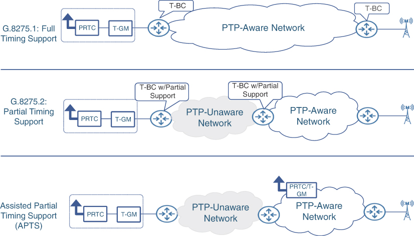
FIGURE 9-13 ITU-T G.8275 Deployment Profiles
Network Time Protocol
Because both NTP and PTP carry timing information over a packetized network infrastructure, a question that network architects often ask themselves is, “Should PTP replace NTP in my network?” The answer to this question is a resounding NO! for a variety of reasons.
NTP has been a widely used timing distribution protocol in communication networks over the past several decades. It has gone through several enhancements over the years to make the protocol more robust and efficient. Not only does NTP have widespread support across vendors and device types, but it is also a lightweight protocol when compared to PTP and does not require expensive hardware. Although the accuracy provided by NTP is magnitudes lower than that of PTP, it is sufficient for its proposed application—that is, to carry the ToD information, accurate in the order of milliseconds. The primary application for ToD in a network is event tracking, where routers and other network devices use the ToD learned through NTP to timestamp the system log (syslog) messages. These syslog messages are used to report a wide range of events such as user login/logoff, configuration changes, protocol-level events, alarms, errors, warnings, and so on. Network management systems make use of this stamping to correlate various events in the network. Given NTP’s widespread use in the networking industry, its (mostly) well-understood nature, and a plethora of reputable sources that cover NTP extensively, this book will not go into the details of NTP operations.
It is expected that NTP will continue to be used for ToD synchronization between network devices for the foreseeable future due to its widespread support across almost all network devices. At the same time, PTP and SyncE will be used to distribute phase and frequency synchronization in 5G-ready mobile xHaul networks.
Summary
During the design phase of a mobile transport network, there is usually a lot of focus on topics such as routing, forwarding, quality of service, and VPN services. Timing and synchronization design and deployment discussions for mobile services have traditionally been an afterthought at best, and justifiably so for the most part.
This chapter explored the importance of distributing timing and synchronization through mobile communication networks. It also examined the reasons why timing and synchronization were considered optional for previous generations of mobile transport networks but is mandatory for next-generation 5G mobile networks. Additionally, this chapter also covers the following topics:
Basic concepts of time and synchronization
Various types of synchronization, such as frequency, phase, and time of day (ToD) synchronization and their relationship to each other
The various sources of clocks and why atomic clocks provide the highest level of accuracy for providing a reference timing signal
The use of the global navigation satellite system (GNSS) and how it can be used to distribute high-quality, accurate time reference to mobile transport networks
The use of Synchronous Ethernet (SyncE) to distribute frequency synchronization across packet networks
Precision Time Protocol (PTP) operations, clock types, reference network, and deployment profiles to distribute phase synchronization through a packet-based mobile transport network
The use of Network Time Protocol (NTP) for distributing ToD synchronization and why NTP cannot replace PTP in mobile networks for the foreseeable future
Timing and synchronization are the final building blocks discussed in this book for designing and deploying 5G-ready mobile transport networks. The next chapter will focus on combining all the essential technologies needed to build a mobile communication network—RAN decomposition and virtualization, 5G Core, mobile xHaul transport, Segment Routing–based transport underlay, data center networking, VPN services, and time synchronization—and how to use these individual technologies to create a cohesive, end-to-end 5G network design.
References
1. 3GPP Technical Specification 38.104, “NR; Base Station (BS) radio transmission and reception,” https://www.3gpp.org/ (last visited: Mar 2022)
2. ITU-T G.8261, “Timing and synchronization aspects in packet networks,” https://www.itu.int/ (last visited: Mar 2022)
3. 3GPP Technical Specification 38.104, op, cit.
4. National Institute of Standards and Technology (NIST) F1 Cesium Fountain Atomic Clock, https://www.nist.gov/ (last visited: Mar 2022)
5. Bureau International des Poids et Mesures (BIPM): Time Department, https://www.bipm.org/en/home (last visited: Mar 2022)
6. GPS Accuracy, https://www.gps.gov/ (last visited: Mar 2022)
7. “5G is all in the timing,” Ericsson, https://www.ericsson.com/ (last visited: Mar 2022)
8. Galileo Initial Services, https://www.euspa.europa.eu/ (last visited: Mar 2022)
9. Microsemi, https://www.microsemi.com/ (last visited: Mar 2022)
10. “Configuring the Global Navigation Satellite System,” Cisco, https://www.cisco.com/ (last visited: Mar 2022)
11. “Resilient Navigation and Timing Foundation,” https://rntfnd.org (last visited: Mar 2022)
12. Cisco NCS540 front panel, https://www.cisco.com/ (last visited: Mar 2022)
13. Juniper ACX500 front panel, https://www.juniper.net (last visited: Mar 2022)
14. Rec. ITU-T G.8261.1, “Packet delay variation network limits applicable to packet-based methods (Frequency synchronization),” https://www.itu.int/ (last visited: November 2021)
15. ITU-T G.8264, “Distribution of timing information through packet networks,” https://www.itu.int/ (last visited: Mar 2022)
16. RFC 1059, “Network Time Protocol (Version 1) Specification and Implementation,” https://www.ieee.org/ (last visited: Mar 2022)
17. Dennis Hagarty, Shahid Ajmeri, and Anshul Tanwar, Synchronizing 5G Mobile Networks (Hoboken, NJ: Cisco Press, 2021).
18. Ibid.
19. O-RAN Synchronization Architecture and Solution Specification 1.0, https://www.o-ran.org/ specifications (last visited: Mar 2022)
20. ITU-T G.8273.2, “Timing characteristics of telecom boundary clocks and telecom time slave clocks for use with full timing support from the network,” https://www.itu.int/ (last visited: Mar 2022)