
Chapter 6
Emerging Technologies for 5G-Ready Networks: Segment Routing
As discussed thus far, mobile communication networks have evolved significantly since their introduction in the 1970s. In the same timeframe, transport networks have gone through technological advances of their own and have brought the latest transport technology into mobile communication networks (MCNs) to provide reliable and effective connectivity between cell sites and the mobile core. These mobile transport networks have evolved from T1/E1 in the early days of MCNs, to ATM and Frame Relay in the second generation, and finally to an all-IP transport in the third and fourth generations of mobile networks. With more recent enhancements in the radio access network (RAN) and mobile core, the traditional mobile backhaul (MBH) has also seen a move toward a more sophisticated xHaul network. In parallel to all these changes, and given the shift toward software-defined transport, there is also a desire to incorporate network programmability into mobile transport.
Today, IP- and MPLS-based transport networks make up the bulk of all MBH deployments. Being more than two decades old, Multiprotocol Label Switching (MPLS) has become a versatile protocol with a multitude of features and custom knobs. The enhanced functionality comes at the expense of added complexity, however, primarily through augmentation of multiple features and functions in existing network architectures.
Mobile network operators demand simplicity with a higher degree of programmability and control over traffic in the transport network. Segment Routing is one of the emerging transport technologies that promises to remove a lot of complexity, while at the same time offering network programmability and integration with higher-layer application, which have become critical in the next generation of transport networks.
Complexity in Today’s Network
Since its inception in the late 1990s, MPLS has been widely adopted as the transport technology of choice, becoming the bedrock of virtually all large-scale networks, including transport for MCN. It borrows the old ATM and Frame Relay concepts of traffic switching, quality of service (QoS), and path-based traffic forwarding, while adapting them for IP transport. MPLS works by encapsulating IP data within a 4-byte label, which is pushed on the IP packet at the source router. This label is used to make forwarding decisions by routers along the label switched path (LSP), where every transit router examines the label information, compares it with its own forwarding information base (FIB), swaps the label with the new forwarding information (that is, the new label), and forwards it toward the destination. It can also impose (push) or remove (pop) labels according to the local FIB. An IP and routing table lookup is not performed during the forwarding process, making MPLS a Layer 2.5 technology according to the Open Systems Interconnect (OSI) model.
MPLS was originally designed for fast packet switching in core networks, and later offered additional value through traffic engineering, fast reroute, and virtual private network (MPLS-VPN) capabilities. MPLS technology makes use of purpose-built protocols to provide extensibility and flexibility, which has allowed it to keep up with the growing traffic patterns and network evolution for over two decades. For instance, in addition to the IGP for route and topology distribution, Label Distribution Protocol (LDP) is used to propagate label information through the network, and Resource Reservation Protocol (RSVP) is needed to provide traffic engineering capabilities. The trade-off, however, is that the use of each additional protocol adds a layer of complexity as well as contributes to scalability limitations on the routers running these protocols. In order to exchange labels, every router establishes and maintains an LDP adjacency with each one of its neighboring routers. This TCP-based adjacency is in addition to any Interior Gateway Protocol (IGP) and Border Gateway Protocol (BGP) adjacencies that the router might already have, using memory and CPU resources as well as contributing to network traffic in the form of periodic hellos. RSVP, used to provide traffic engineering and bandwidth reservation for services throughout the network and thus called RSVP-TE, is even more taxing on routers’ resources than LDP. For RSVP-TE to work, every router along the path (called midpoints) must be aware of how to forward the traffic based on the traffic engineering or bandwidth requirements established at the source—also called the headend. Over the last several years as networks grew larger and traffic engineering was deployed to ensure guaranteed bandwidth or assured path, midpoint scaling has emerged as a major resource strain and scalability roadblock. Although MPLS has enabled a number of value-added services for the transport network over the past quarter century, what was once a revolutionary and exciting innovation now seems cumbersome and too complicated to operate and manage with all the add-ons.
The biggest challenge for MPLS as the transport protocol of choice emerged when it gained a foothold in access networks such as MBH. As explained earlier in Chapter 3, “Mobile Networks Today,” MPLS-based services are established using a router’s host route without summarization—relatively easy to accomplish within a smaller domain (such as the IP Core) comprising a relatively small number of routers. However, when implemented in access networks such as MBH, where device numbers can range in the hundreds of thousands of nodes that require connectivity across multiple access, aggregation and core domains, scalability challenges start to emerge. The introduction of Seamless MPLS architectures, using a combination of IGP, careful route filtering, and enhancements in BGP to carry label information, as defined in RFC 3107, enabled mobile network operators to circumvent the scalability challenges and deploy MPLS in some of the world’s largest mobile communication networks with 200K cell sites.1
Despite being more than a decade old and one of the most deployed backhaul architectures, however, Seamless MPLS concepts remain too complex for some. The layers of reachability defined in the Seamless MPLS architecture—IGP within each domain, BGP across domains through next-hop self-manipulation—present a complicated solution, which was discussed earlier in Chapter 3. It requires a deep and thorough understanding of the interworking of multiple communication protocols for any network architect designing an MPLS-enabled backhaul or any operations engineer troubleshooting connectivity issues to navigate through the multiple layers of reachability. Simply put, the Seamless MPLS architectural framework provides scalability and uniformity across domains but is high maintenance and complex to design, manage, and operate.
Introducing Segment Routing
In everyday life, a path to a destination can be described in different ways. for example, “walk to the intersection of streets A and B and walk east for one block,” or “hop on a bus number X, get off at the railway station, and take a train to city Y.” Each of these path examples can be dissected into individual segments; for example, “walk to the intersection of streets A and B” is the first segment and “walk east for one block” is another one. These are examples of predetermined routing decisions made at the source. Segment Routing (SR) relies on a similar concept—it uses a collection of segments, or rather instructions, that make up the entire path to reach the destinations. This information is added to the traffic at the source, before it’s passed on to a data network that is capable of understanding and acting upon these instructions.
SR addresses the complexities and challenges that were faced in Seamless MPLS-based networks and offers a simplified, SDN-friendly, scalable solution that could help scale services offered by the data network. Its simplicity and ease of implementation have made it gain popularity and become a favored choice for service-oriented data networks, such as an xHaul transport network in an MCN. Figure 6-1 shows a simple, end-to-end overview of the use of SR in a mobile transport network providing connectivity between cell sites and the 5G Core.

FIGURE 6-1 Segment Routing in Mobile Communication Networks
Concept of Source Routing and Segments
Source routing has always been desirable, as the data source is often the most informed entity about the preferred or required treatment for the data it generates; however, implementing source routing in an IP network would have meant using IP options in the header. This could support only a limited number of hops as well as make the IP header bulky and inefficient to parse. It also requires a holistic view of the network topology and link states, whereas typical IP routing protocols provide only the next-hop information. Hence, source routing is neither efficient nor easy to achieve because, without the appropriate knowledge of the data network that has to transport this traffic or the ability to influence those data paths, very little could be done at the source to control the destiny of data. Mechanisms such as QoS marking, traffic engineering, and policy-based routing (PBR) have been used to exert some amount of control, but all of these have their own drawbacks and limitations. QoS markings allow the source to request a specific traffic treatment; however, this requires a hop-by-hop QoS definition across the entire network to classify and honor those markings. PBR can be used to match against a specific source attribute, overriding the global routing table, but it, too, has to be defined on every transit router and hence is not practical for influencing the end-to-end traffic path. Traffic engineering, commonly implemented using MPLS, also faces many challenges discussed in previous sections.
So, it’s no surprise that all dynamic routing protocols implemented today use traffic destination information to make forwarding decisions. These protocols depend on best path calculations using various metrics and forward traffic toward the next hop, with the expectation that the subsequent hop knows what to do next. The applications sourcing the traffic have no visibility of the topology and no control or influence over the decision-making process for the path used. It’s technically possible to define a source-routed path on the application itself, which in case of an MCN could be the subscriber’s mobile devices. This, however, poses a security threat, as these applications and data sources reside outside the service provider’s trust boundary. As such, any decision to influence the traffic path within an SP network must be delegated to the equipment within the trusted network and with appropriate topology information, such as the CSR or IP routers in the 5GC domain.
Segment Routing (SR) includes the path instructions in the packet itself at the source and, hence, in essence uses the concept of source routing.2 It offers a much simplified and scalable mechanism to achieve this while still leveraging the dynamic destination-based routing of the network, and at the same time instructing the transit routers of the desired behavior. These instructions, called segments, are defined in the RFC as follows: “A segment can represent any instruction, topological or service based.”3 The segments can therefore represent a link, a networking node (router), a portion of the traffic path, a specific forwarding instruction, a particular traffic treatment, or a combination of these. Segments can vary in the level of detail and can be very precise, defining the exact routers and links that the traffic should take, or they can be loosely defined to ensure that specific routers or links are in the path used to reach the destination. Connecting back to the analogy of directions used by humans to reach a destination, each part of an instruction can be considered a segment, and the specific details of how to reach the end of a segment may be omitted and left for the person to pick any available option. Similarly, in SR, the segments might require that a certain router (which might not be the preferred next hop based on dynamic routing) be reached, while not necessarily enforcing the exact link or intermediate node to reach that router.
Segment IDs (SIDs) and Their Types
To distinguish between segment instructions, an SR-capable device relies on special identifiers, called segment identifiers (segment IDs, or SIDs for short). Although the term SID pertains to the identifier of a segment rather than the segment itself, the industry uses the term to describe both segments and their respective identifiers. The term SID will be used in both senses throughout this book, unless the difference is highlighted.
When we take a closer look at the path analogy from the previous section, it is possible to observe that some segment instructions can be recognized and executed at any starting point (“walk to the intersection of streets A and B”); thus, these have global significance. Others are relative, or locally significant, and can only be executed from a very specific position (for example, “walk east for one block”). While the latter can potentially be executed anywhere, it will hardly result in the desired outcome, if not done at the specific location. SR uses the same concept and distinguishes globally significant, or global SIDs, and locally significant, or local SIDs.
For the SR-capable routers to act according to the instruction encoded in the SID, it has to be expressed in the transmitted packet. At the time of publication, two main approaches exist:
SR-MPLS: Uses MPLS labels to express SIDs.
SRv6: Uses the IPv6 destination address field and additional IPv6 routing headers to express SIDs.4, 5
Figure 6-2 shows the SID expression in SR-MPLS and SRv6 packets. The SRv6 concepts will be introduced later in this chapter, while this section’s focus is on SR-MPLS.

FIGURE 6-2 Segment ID (SID) Representation in SR-MPLS and SRv6
A number of different segment types and SIDs are defined by the Segment Routing Architecture IETF standard; some are global, while others have local significance:6
Prefix-SID: This is one of the most common SIDs used in SR and serves as an identifier for the IGP-Prefix segment, an instruction to reach a specific IGP prefix. How this IGP prefix is reached is not explicitly specified, and if multiple equal-cost paths to this prefix exist, all of them can be used simultaneously; that is, Equal Cost Multi Path (ECMP) is used. The Prefix-SID is a global SID and can be recognized by any SR-capable router in an IGP domain. It is akin to an instruction such as “walk to the intersection of streets A and B.”
Node-SID: This is a type of the Prefix-SID and therefore is also globally significant. It represents an IGP prefix uniquely identifying a node, which is usually the router’s loopback interface.
Anycast-SID: This is another type of the Prefix-SID and is tied to an IGP prefix announced by multiple nodes in the same IGP domain. Anycast-SID is a global SID and is used to instruct an SR-capable router to forward a packet to the closest originator of the Anycast IP prefix. In everyday life, this instruction type is similar to “drive to any of the closest gas stations.”
Adjacency-SID (or Adj-SID for short): This is an example of a local SID. This SID identifies a router’s particular IGP adjacency, persuading the router to forward a packet over this adjacency, regardless of a best path installed in the routing table. Applying SR jargon to the original “walking” analogy, the Adj-SID would be the “walk east for one block” segment.
Binding-SID: This identifies an instruction to forward a packet over a Segment Routing Traffic Engineered (SR-TE) path or, using SR jargon, an SR policy. The SR traffic engineering concepts and constructs will be covered in the upcoming sections of this chapter. Binding-SID is equivalent to taking a predetermined bus route from a bus station. Although Binding-SID can be implemented either as a local SID or a global SID, at press time, most of the Binding-SID implementations are locally significant.
BGP Prefix-SID: This can be used in scenarios where BGP is used to distribute routing information. BGP Prefix-SID is very similar to the Prefix-SID but is bound to a BGP prefix and has global significance.7
The next few SID types belong to segments used in BGP Egress Peering Engineering (BGP EPE), an approach defined in the Segment Routing EPE BGP-LS Extensions IETF draft.8 In simple terms, BGP EPE applies concepts of SR to BGP peering in order to forward packets toward a specific BGP peer, or a set of peers. Expanding the original human analogy to this case, the use of BGP EPE segments can be viewed as an instruction to change transportation authority and hop off the bus to take a train to the final destination. A few different types of BGP EPE SIDs are defined the Segment Routing Architecture IETF standard:9
BGP PeerNode-SID: This instructs a router to forward a packet to a specific BGP peer, regardless of the BGP best path. By using this SID type, a packet source can define the autonomous system (AS) exit point. However, being a local SID, the BGP PeerNode-SID allows the use of any adjacency toward the BGP peer.
BGP PeerAdj-SID: In contrast, this is used to specifically define which adjacency or link has to be used to forward a packet to the BGP peer.
BGP PeerSet-SID: This is another form of BGP EPE SID and is used to designate a set of BGP peers, eligible for packet forwarding. Because the BGP PeerSet-SID can identify more than one BGP peer, a load-balancing mechanism can be used to forward packets toward these BGP peers.
With the growing list of SR adopters, new use cases for Segment Routing may emerge requiring new SID types. The list of SIDs presented in this section is not exhaustive and will likely expand. Figure 6-3 provides an example of different SID types in SR-MPLS networks.

FIGURE 6-3 Segment ID Examples
Another characteristic feature of Segment Routing is its elegant approach to the distribution of instructions or SIDs throughout the network. In an effort to simplify network design and implementation, SR does not rely on additional protocols but rather leverages the existing IGP or BGP protocols instead. Figure 6-4 highlights the simplification brought in by SR, as compared to existing Seamless MPLS architectures, and shows how SR simplifies the protocol stack by leveraging existing routing protocols to perform functions other than basic reachability and connectivity. The SR implementation of these functions is discussed in subsequent sections.
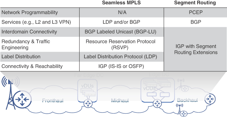
FIGURE 6-4 Protocol Stack Simplification with Segment Routing
Defining and Distributing Segment Information
In a typical network, information such as router’s capabilities, prefixes, adjacencies between the routers, and link attributes are distributed by an Interior Gateway Protocol (IGP). The popular IGPs used by service providers are designed to be friendly for functionality expansion and use type-length-value (TLV) tuples to carry chunks of information within IGP data units. Allowing an IGP to carry additional information about routers or their links is only a matter of adding new TLVs or sub-TLVs to the protocols’ specification. A few IETF RFCs propose adding SR extensions to the three popular IGPs: namely, RFC 8667 for ISIS, RFC 8665 for OSPF, and RFC 8666 for OSPFv3.10, 11, 12 In essence, all these RFCs propose additional TLVs and sub-TLVs to propagate SR Prefix-SIDs along with the prefix information, Adjacency-SIDs with information describing adjacencies, as well as some non-SID information required for SR operation.
Unlike traditional MPLS implementations, where labels are always locally significant (with the exception for some special use labels), SR heavily relies on the use of global SIDs, which require special precautions in the case of SR-MPLS. Indeed, a global SID should have the same meaning on all the nodes in a particular domain; therefore, if the SID value is expressed as an MPLS label, either this label must be available on every node or another form of unambiguous mapping of this SID to the label that’s understood by the downstream devices should exist.
Suppose a prefix of 10.0.0.1/32 is propagated throughout the domain and has a corresponding Prefix-SID, represented by an MPLS label 16001. It is not always reasonable to assume that this MPLS label is available on all the nodes in the domain. This MPLS label may already be in use by some other protocol, or outside the label range supported by the device, and thus cannot be used by SR-MPLS. The problem is easily solved if the Prefix-SID or any other global SID is propagated as a value relative to some base, instead of the actual label. This relative value is called an index, and the base with the range allocated for SR global SIDs becomes a Segment Routing Global Block (SRGB). Each node can then advertise its own SRGB, allowing neighbors to correctly construct MPLS labels mapped to the global SIDs by this node. Put simply, if the Prefix-SID of 10.0.0.1/32 is propagated as an index of 1, it is translated to an MPLS label of 16001, provided that the downstream neighbor’s SRGB starts at 16000. Standards allow SID distribution as both an index or actual value; however, current implementation uses an index for Prefix-SIDs and the actual value for Adjacency-SIDs.
The distribution of Adjacency-SIDs as values is particularly interesting, as the standard also defines a Segment Routing Local Block (SRLB) to be used for some types of local SIDs. Although Adj-SID is a local SID, the adjacency itself is always unique and thus does not require any coordinated use of a particular value across multiple nodes. A node can simply allocate a label from its dynamic label space and propagate it as a value because no other node is required to have this local label installed in the FIB. The proposed use of SRLB is rather for locally significant but non-unique intent, such as “forward a packet to a locally attached scrubber” or something similar.
Another important type of non-SID information propagated by IGP and worth mentioning is the SR algorithms supported by a node. Any SR-capable node supports at least one algorithm—Shortest Path First (SPF), which is the same algorithm used by IGPs without SR extensions. SPF is the default algorithm used in SR, but other algorithms may be supported as well. For example, the Strict SPF algorithm may be supported by default, based on vendor’s implementation. Simply put, Strict SPF is the same as regular SPF, with one exception: it does not allow any transit node to redirect the packet from SPF path. By using Strict SPF, the source can be sure that a packet does not deviate from the intended path due to a local policy on a transit node. Other types of SR algorithms can also be defined and are generally known as flexible algorithms. SR flexible algorithms are discussed later in this chapter.
Another example of non-SID information required by SR is the Maximum SID Depth (MSD) supported by a node. The MSD is valuable in SR-TE scenarios, where a list of SIDs expressed in an MPLS label stack might exceed the capabilities of some platforms. If every node’s MSD is known, the end-to-end path can be calculated using the allowed number of SIDs.
In ISIS, most non-SID information is carried in sub-TLVs under Router Capability TLV. Prefix-SIDs are propagated as sub-TLVs under Extended IP Reachability TLV, along with multiple flags and algorithm field tying the Prefix-SID to a particular algorithm (SPF, Strict SPF, or flexible algorithms). Finally, Adj-SIDs are propagated under the Extended IS reachability TLV using sub-TLVs defined for this purpose. Figure 6-5 illustrates an example of an ISIS packet capture with SR extensions.

FIGURE 6-5 ISIS Extensions for Segment Routing Example
OSPF carries similar sub-TLVs in various Type 10 Opaque LSAs. Non-SID SR information is flooded in the Router Information Opaque LSA, while the Prefix-SID and Adj-SIDs are transported as sub-TLVs in the Extended Prefix Opaque LSA and Extended Link Opaque LSA, respectively.
Although IGP has the most comprehensive set of SR extensions, it is possible to propagate SR information using Border Gateway Protocol (BGP) as well. BGP is a highly flexible protocol and a popular choice to convey routing information not only between autonomous systems but within many data centers as well. The RFC 8669 defines a new optional transitive path attribute to transport both the Prefix-SID label index and originator’s SRGB range. This BGP Prefix-SID path attribute can be attached to BGP labeled Unicast prefixes and used to distribute SR information across the network.13
Segment Routing Traffic Engineering (SR-TE)
Growing network complexities, exploding traffic volumes, and diverse traffic types have rendered networks using only the SPF algorithm to calculate optimal paths inadequate. Because network links are expensive assets, service providers wish to utilize them as much as possible; however, in many cases, they remain idle and not generating revenue. An attempt to reclaim these idle or underutilized links and transport appropriate traffic types over them has created a new field of networking—traffic engineering (TE). TE brings innovative approaches to steer traffic over a vast number of potential paths through the network, improving the overall efficiency of network resources utilization, reducing the cost of transportation for critical and sensitive traffic, and offering a customized forwarding path for certain traffic types.
Current Approach to Traffic Engineering
In a way, rudimentary TE capabilities were offered by routing protocols via link metric manipulation. Due to its nature, however, metric manipulation affects all traffic types; hence, instead of distributing, it shifts all traffic flows without adding much improvement in network resources utilization efficiency. However, when mixed with strategically provisioned logical tunnels, acting as pseudo-links between a few network nodes, static routing or PBR enables achieving some degree of traffic distribution over multiple paths. Unfortunately, when IP-based logical tunnels are used, such as Generic Routing Encapsulation (GRE), this poses a risk of routing instabilities and potential routing loops, as IP-based tunnels can be easily affected by interaction with static routing and metric changes in routing protocols. Although this method still remains in a network architect’s tool inventory, more sophisticated and powerful methods were invented to comply with demanding service level agreements (SLAs) and provide granular control over different traffic types as well as optimal link utilization in complex and large topologies.
The MPLS forwarding plane created an opportunity to take the tunnel-based approach to a whole new level. A labeled switch path (LSP), an equivalent of a tunnel, can be established in the MPLS forwarding plane by programming an appropriate state on each node along the desired path. Every node along this path would need to allocate a special label associated with that LSP, and the packet received with this label at the top will be forwarded down the LSP.
Normally, traffic is steered into an LSP at the headend node by various methods. Some of these methods include preferential use of labeled paths over regular Routing Information Base (RIB) entries to reach BGP next hop(s), special IGP tweaks, and static routing. Once the decision to steer the packet into an LSP is made, an MPLS label is pushed on top of this packet, and it is forwarded along the LSP.
Forwarding a packet along the LSP means sending a packet to the immediate downstream neighbor over a specific adjacency. Before the packet hits the link toward the next downstream node, the ingress label is typically swapped with a label assigned to the same LSP by a downstream node. The process repeats until the penultimate hop, where a label can be swapped with label zero or removed completely, depending on the configuration. Using this process, a packet can be forwarded along any pre-negotiated path toward the destination, regardless of the result of SPF algorithm calculations for a particular destination, as shown in Figure 6-6. This method is called MPLS-TE, and it proved to be effective in achieving the goals of sending traffic over an engineered path. MPLS-TE is currently a widely deployed technique in many service provider and enterprise networks.
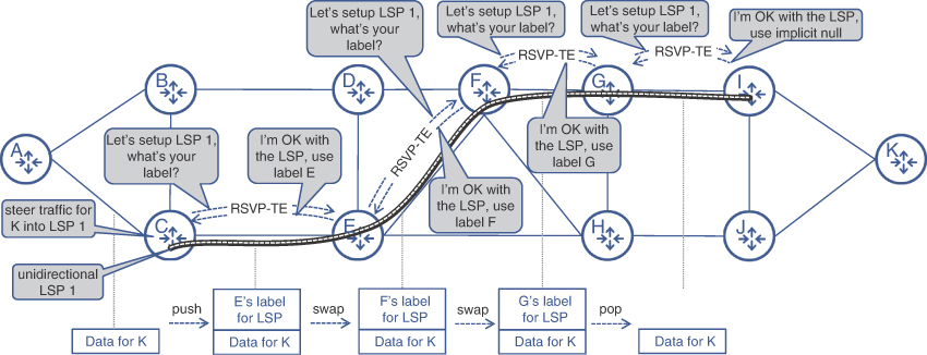
FIGURE 6-6 Example of MPLS-TE LSP Packet Forwarding
The desired path of an LSP can be calculated at the headend node by executing a special version of the SPF algorithm, called Constrained Shortest-Path First (CSPF), on the known network topology. As the name implies, CSPF is based on SPF but uses additional constraints for the calculations, such as “exclude certain links from the topology” or “use special metric for calculations.” While the number of LSPs originating at a particular headend can be significant, with powerful CPUs and ample memory resources, today’s routers can easily cope with all those path calculations. The impact on midpoint nodes, however, can be much more pronounced. Because every node in the path of any LSP has to program and maintain the forwarding state, in large networks a typical midpoint node might be in the path of hundreds of thousands of LSPs, which creates a significant scalability challenge.
Negotiating the use of MPLS labels for each LSP across the network relies on extensions to Resource Reservation Protocol (RSVP), referred to as RSVP-TE.14 The RSVP-TE protocol signals the desired path and secures MPLS labels for LSP hop-by-hop, such that every node down the path is aware and ready to forward traffic down the LSP. If an LSP has special demands, such as a certain level of available bandwidth along the path, RSVP-TE takes care of the bandwidth requests and provides arbitration for the situation when multiple LSPs request more bandwidth than is available at a particular node. These mechanisms come with a price, as the appropriate state has to be created and periodically refreshed on all these nodes, which exacerbates scalability challenges faced by MPLS-TE midpoint nodes. Additionally, these negotiations may impose a delay in establishing an LSP.
Besides scalability challenges, the use of an additional protocol for MPLS-TE operation can bring more network vulnerabilities and requires attention when securing the network perimeter. All of these challenges, combined with increased complexity of deployment, operation, and troubleshooting, create significant backpressure, slowing down the MPLS-TE adoption rate. TE with SR takes a different approach and provides a way around these serious challenges.
Traffic Path Engineering with Segment Routing
TE was an integral part of SR since its very inception. In fact, enabling SR on a network immediately makes it TE-ready—no additional protocols, labels, negotiations, or tunnel maintenance on transit nodes required. Instead, Segment Routing Traffic Engineering (SR-TE) uses SIDs as waypoints. The collection of these waypoints (that is, various types of SIDs) forms a navigation map helping all nodes to send packets along desired paths. A headend, in turn, can craft the path instructions by listing the IDs of all segments a packet has to traverse. The resulting SID-list becomes the path instruction, which can be expressed as an MPLS label stack and pushed on top of a packet. The packet is then forwarded according to the top label, until it reaches the end of the current segment, where the label is popped and the next label becomes active. This process continues, taking the packet through all segments over the desired path, as shown on Figure 6-7, where Router C implements an SR policy toward Router I, which uses the Prefix-SID of Router G as a first waypoint, relying on intermediate routers to implement ECMP wherever possible. Router G forwards traffic to the next waypoint over adjacency to Router I, as prescribed by Router C.

FIGURE 6-7 Example of SR-TE Packet Forwarding
Having the complete set of instructions attached to the packet itself removes the need for label negotiations along the LSP. Because there are no negotiations, no additional protocols are needed and, more importantly, no additional state is created on mid- and endpoints. As far as the midpoint is concerned, all necessary actions are already programmed in its FIB for every MPLS label used by SR, thanks to the routing protocol’s SR extensions. Hence, the midpoint can simply forward packets, sent over SR-TE path, as yet another MPLS packet with no additional per-LSP state created. The same is true for endpoints; however, endpoints typically receive either unlabeled packets or packets with the service label exposed, due to the penultimate hop popping (PHP) behavior.
Without the need to maintain extra state on mid- and endpoints, the SR approach to TE is ultra-scalable. All the necessary state for each SR-TE path is created and maintained on headend nodes, with a major component being the SR-TE path’s SID-list. The SID-list can either be defined statically via configuration, dynamically calculated on the headend itself, or programmed by an external application through APIs (if supported by the headend’s software). The CSPF algorithm is used to calculate the path, applying the desired constraints and optimization criteria on the SR-TE topology database. In SR terminology, the resulting SID-list, combined with some additional parameters, creates an SR policy—the equivalent of an MPLS-TE tunnel.15
Segment Routing TE Policies
Justifiably, there are no references to tunnels in SR-TE jargon, as there is no extra state created at the end of or along the LSP; therefore, no actual tunnels are created. In SR, a packet is forwarded along the desired LSP using instructions attached to the packet itself, typically in the form of MPLS labels. These instructions rather define a policy on how a packet should be forwarded across the network, thus the name SR policy.
SR policy is a construct used to create and attach traffic-forwarding instructions to the packets. This policy defines the intent on how traffic should be treated and forwarded across the network. In a simple scenario, an SR policy is associated with a single SID-list, providing instructions on how to forward packets across the network. When such a SID-list is programmed in the FIB, SR policy is considered to have been instantiated on the headend.
Even the most stable networks are prone to link and node failures thus programmed SID-lists might become obsolete and cause traffic blackholing. This scenario is quite likely in the case of statically defined SID-lists. Yet, even with dynamically calculated SID-lists, it is still plausible that CSPF would not be able to find another path, due to the constraints defined in the SR policy after the failure in the network. To provide more flexibility, SR policies can have more than one candidate path. Each candidate path is paired with a preference value and can prescribe to use a different path for SR policy, if a more preferred candidate path is unavailable. Moreover, each candidate path can have more than one SID-list, each with its own weight. When a candidate path with multiple SID-lists is active, the traffic is load-balanced across these SID-lists based on the ratio of their weights, as shown on Figure 6-8.16 Only one candidate path can be active at a time for a given SR policy, and if none of the candidate paths are valid, the whole SR policy becomes invalid and is removed from the forwarding table.
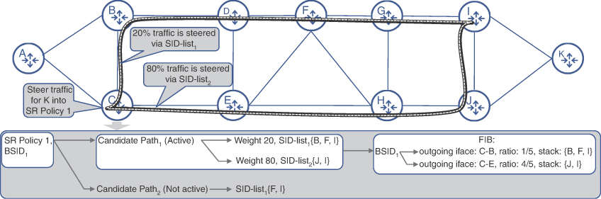
FIGURE 6-8 SR Policy Construct
Depending on communication flows, a significant number of SR policies can be programmed on each individual headend node, let alone in the whole network. It is entirely possible to have multiple SR policies with different paths, or otherwise different traffic treatment, between a given headend and endpoint pair. Thus, every SR policy cannot be differentiated based only on the headend–endpoint pair but requires an additional parameter for proper identification. This parameter is color—an arbitrary 32-bit number used to form the tuple (headend, color, endpoint) that uniquely identifies the SR policy in the network.17 Oftentimes, color is also used to identify the intent (that is, it can represent how traffic will be treated by the network) and can further be connected to specific SLAs such as Gold, Silver, and Bronze traffic types.
When instantiated, each SR policy is assigned its own binding SID (BSID), which is one of the primary mechanisms to steer traffic into the SR policy. Typically, the BSID is locally significant and is swapped with a stack of labels representing the SR policy’s active SID-list, effectively steering a packet labeled with BSID into its respective SR policy. The use of BSID is not the only available mechanism for traffic steering, however, as seen in the next section.
Traffic-Steering Mechanisms
The most straightforward approach to steer traffic into an SR policy is to use a BSID, but it requires an upstream node to impose the BSID on top of the packet. When a packet with the BSID arrives on the node with the SR policy instantiated, the BSID is expanded into the SR policy’s actual SID-list. In addition to the BSID, a few other mechanisms exist to steer traffic in the SR policy locally.
Although it depends on the vendor’s implementation, one obvious way to steer traffic locally into the SR policy is to use static routing (altering routing table pointers); however, such direct use of static routing doesn’t scale very well.
A modified version of static routing, or rather routing table tweaking, is used to steer traffic flows into SR policies. In many cases, it might be desirable that traffic flows for destinations beyond the endpoint of an SR policy be steered into that SR policy. To accomplish this, a node instantiating the SR policy tweaks its routing table to point to this SR policy as its outgoing interface for any prefixes that are advertised by nodes beyond the SR policy’s endpoint. In some implementations, it is even possible to identify a set of prefixes that are eligible for this behavior, thus limiting the traffic flows automatically steered into the SR policy. Cisco routers implement this behavior under the name of autoroute.
Another, even more scalable and flexible approach is to use the color of the SR policy for automated steering. Automated steering is the go-to solution in environments with services connected via BGP L2 and L3 VPNs. These VPN services rely on a potentially large number of service prefixes advertised by provider edge (PE) routers. This approach normally results in the color being attached to a prefix as a special BGP Color Extended Community defined in the IETF draft Advertising Segment Routing Policies in BGP.18 The 32-bit color value in the Color Extended Community is used to form a tuple (headend, color, prefix’s BGP next hop). This tuple is then compared with the active SR policies’ identifying tuples on this headend. The active SR policy with the matching color and endpoint (the headend value always matches for obvious reasons) is then used to forward traffic destined to this BGP prefix. This automated steering solution works for both service (VPN) and transport routes.19 Figure 6-9 shows both automated steering and autoroute mechanisms.

FIGURE 6-9 Steering Traffic Flows into SR Policy
This automated steering approach can be combined with an automated SR policy instantiation mechanism in a feature known as On-Demand Next Hop (ODN). In addition to automated traffic steering into matching active SR policies, ODN can create and instantiate SR policies if a matching SR policy does not exist. ODN uses BGP next-hop as an endpoint and the value from Color Extended Community as the SR policy’s color. Depending on the vendor’s implementation, some form of color authorization may be present on the headend, as well as some form of SR policy templates defining optimization criteria and constraints for each color. Put simply, an ODN template removes the need for configuring a separate SRTE policy for destinations that share the same policy constraints. With color authorized through the ODN policy template, any BGP prefix with matching Color Extended Community attribute will result in an automatic SR policy instantiation toward its next hop.
ODN offers a highly scalable solution, removing the need to provision and instantiate a mesh of SR policies between PE routers in advance. Use of this feature can greatly reduce management overhead and operational complexity in a typical MCN with its numerous cell sites-given that there is a need to establish connectivity between cell sites (for Xn communications) as well as between cell sites and the Mobile Core. CSRs can now be configured with only a handful of SR policy templates, allowing ODN to instantiate SR policies to the remote nodes that are advertising service routes with appropriate colors. Figure 6-10 illustrates an overview of ODN operation.
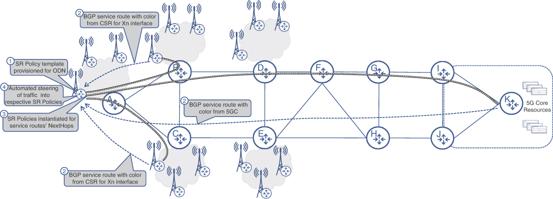
FIGURE 6-10 ODN Operation Overview
Software-Defined Transport with Segment Routing
In everyday life, a commuter might rely on map applications (Google Maps, Apple Maps, and so on) to learn the most optimal route to a destination. Even though the shortest route to the destination may already be known, the state of traffic, congestion, and road closures might result in a different route being faster or better. The cloud-based map application, with better overall visibility of these variables, can therefore provide a better path at that instant. Similarly, in a data network, even though the routing protocols would have already calculated the shortest path, these protocols are not designed to dynamically optimize the path based on network utilization and constraints other than IGP metric. If an external controller has full view of the network’s topology, applicable constraints, current state of links, and possibly their utilization, it can then make a more informed and better decision about the traffic path compared to the dynamic routing protocols. The network utilization and efficiency can be significantly improved, provided this controller can influence the traffic’s path in the transport network, rerouting it through its computed path. It is this idea that led to software-defined networking (SDN), which has gained a lot traction in the last few years and has now become an important part of any network architecture, especially in service provider networks.
At the time SDN started to gain popularity, almost a decade ago, MPLS-TE was already being used to override IGP-computed routing paths in transport networks. Although it could be adapted and used in software-defined transport, MPLS-TE was not invented with SDN in mind. Its scalability limitations, in addition to the slow reaction time to establish a TE tunnel, didn’t make it a very convincing choice for transport SDN. In contrast, SR-TE, a new entrant, presented itself as a viable alternative to MPLS-TE for implementing software-defined transport.
Building Blocks for Software-Defined Transport
The controller performing the brain functions of the software-defined transport, generally called an SDN controller, would need to learn sufficient information about the network. At a bare minimum, it would need to be aware of the full network topology as well as any changes occurring in it, such as link or node failures. Additionally, its path computation can be more accurate if it has real-time information, such as link utilization, latency of the links, allocated bandwidth over a link, constraints and affinity associated with the links, type of links (encrypted vs. unencrypted), and so on. The controller will also need to be able to communicate the path decisions to the network devices.
None of the existing protocols could fulfill these requirements. Hence, implementation of SDN for transport networks gave birth to the following new protocols and functions that could facilitate the implementation of its concepts and methods:
Path Computation Element (PCE)
BGP Link State (BGP-LS)
Path Computation Element Communication Protocol (PCEP)
These protocols and functions will be discussed next.
Path Computation Element (PCE)
The SDN controller used by SR-TE is called the path computation element (PCE).20 Although the PCE was not defined exclusively for SR-TE, it has become the de facto transport SDN controller used across the networking vendors. The PCE relies on a hybrid SDN model rather than completely removing intelligence from the forwarding devices. In fact, by definition, the PCE functionality can be implemented on the forwarding device directly, instead of being deployed externally. Irrespective of the deployment model used, the following are the three key functions a PCE is meant to perform:
Topology collection: As highlighted earlier, topology awareness is a primary requirement for the SDN controller to be able to compute the desired path. Hence, the PCE should be able to learn this information from the network. One protocol of choice for topology collection is BGP-LS, discussed in the section that follows.
Path computation algorithms: In MPLS-TE networks, the headend was responsible for path computation using its limited topological awareness. In SDN-based transport, this function of Constraint-based Shortest Path First (CSPF) computation is delegated to the PCE.
Communication with the headend: The PCE should be able to receive a path computation request from the headend router, which now acts as a client to the PCE and is referred to as the path computation client (PCC). Consequently, the PCE should be able to communicate the computed path to the PCC. Since none of the existing protocols provided the capability for such message exchange, a new protocol called PCE Communication Protocol (PCEP) was defined to fill the void.21 PCEP will be discussed in detail in the next section.
BGP Link State (BGP-LS)
Both of the protocols that are predominantly used in transport networks (OSPF and ISIS) are link-state protocols, and hence the routing database for these contains complete information about the links, nodes, and prefixes that build the network. Additionally, through the use of SR extensions, these protocols also communicate SR-related information such as SID values, SRGB, and SRLB ranges, as well as SPF algorithms being used by a router. In MPLS-TE, the link-state information from the IGPs was used to populate a traffic engineering database (TED) utilized by the headend nodes to compute the TE path.
One apparently simple way for the PCE to learn the TED information is by making it part of the IGP domain. This would enable the PCE to learn the IGP link-state information directly and generate the TED. A challenge with this approach, however, is that a typical large-scale transport network is composed of multiple IGP domains. The link-state information, including the SR-related extensions, is not meant to be propagated across IGP domain boundaries—this would have defied the purpose of creating these domains. Hence, by only participating in IGP, the PCE’s visibility will be limited to only one domain. Even if the PCE resides in IGP’s backbone (Area-0 in OSPF or level-2 ISIS), it can only learn the prefixes (and not the link states and SR details) from other areas due to the nature of IGP.
Therefore, for gathering and sharing the TED with the PCE, a new method was required. BGP, being a scalable and efficient protocol for bulk updates, was chosen for this, and a new BGP Network Layer Reachability Information (BGP NLRI) was defined to carry TED information.22 Known as BGP Link State (BGP-LS), this address family uses BGP peering between the PCE and the IGP network to gather and provide the full picture of the network to the PCE.
The area border routers are typically used as the BGP peering points and source of link-state information, thus reducing the number of BGP-LS sessions. Furthermore, BGP-LS can leverage the existing BGP route reflector hierarchy for scalability and high availability.
Path Computation Element Communication Protocol (PCEP)
As hinted earlier, the PCE and the PCC need to communicate for exchanging path computation requests and responses. PCE Communication Protocol (PCEP) provides the capability for this communication between PCC and PCE.23 Just like PCE, the definition of PCEP pre-dates SRTE, and hence PCEP can be also used for SDN-type implementation for MPLS-TE. However, the widespread use and deployment of this protocol has been for SR-TE. In addition to the basic functions mentioned, PCEP is also used for the PCC to discover the PCE, carry periodic keepalive messages between them to ensure connectivity, event notification exchange, and error messages related to path computation. The PCE may also use PCEP to initiate a policy that hasn’t been requested by the PCC but rather initiated by an external application.
Application Integration with Transport Network
The need for traffic engineering has always been driven by applications, as it’s the applications that require a certain SLA. However, while leveraging an SDN framework, instead of applications directly interacting with the network elements, the PCE acts as an abstraction of the underlying network, providing a communication medium between the application and the transport network. To work coherently with external applications, the PCE is expected to provide a northbound API interface. Figure 6-11 illustrates the transport SDN building blocks and their operation in a Segment Routing network.

FIGURE 6-11 Overview of Software-Defined Transport Network
While it’s the application that dictates the traffic policy, it uses this API interface to communicate those requirements and constraints to the PCE. The PCE is then responsible for computing the path based on those constraints, communicating that path information to the PCC, and maintaining the path. In some cases, the applications may even override the PCE’s computation function and instead provide a pre-computed path for the PCE to implement on the network.
Some networking vendors might choose to integrate the PCE functions and applications together as a single product offering. For example, Juniper Network’s Northstar Controller boasts of capabilities such as topology visualization, analytics, and real-time monitoring—thus reducing the need for an additional external application.25 Similarly, Cisco’s Crosswork Optimization Engine adds visualization to the PCE functions, while delegating detailed analytics to closely knit external applications that are part of the Cisco Crosswork Cluster.26
5G Transport Network Slicing
Perhaps one of the most promising new concepts introduced in 5G is that of network slicing, which allows a mobile service provider to offer differentiated services to a particular traffic type or an enterprise customer. Traditionally, providing special treatment to traffic types has been synonymous with quality of service (QoS), and although QoS is one of the tools within the slicing toolkit, a network slice is defined end-to-end rather than a per-hop behavior like QoS. This end-to-end network slice, spanning across the MCN domains, is identified using a network slice instance (NSI). Each of the MCN domains uses its respective technology toolkit to implement a corresponding subnetwork slice identified by a network slice subnet instance (NSSI).27 These subnetwork slice instances within various domains combine together to form an end-to-end NSI, as shown in Figure 6-12.

FIGURE 6-12 A Network Slice Instance
The set of technical tools in the RAN and 5GC networks may allow an NSI to use its own dedicated UPF and antennas as well provide its own QoS classification. However, it is the transport network that offers a rich and diverse set of capabilities to complete an end-to-end slice by implementing network functions to comply with the slicing requirement imposed by the NSI. One such capability is the use of an SDN controller, as mentioned in the previous section, to administer end-to-end transport slices by using SR-TE policies. Transport network slices might not have a 1:1 correlation with RAN or 5GC slices, and in most cases might not even be aware of the slices in those two domains. However, the transport domain’s role is instrumental in ensuring the end-to-end slicing requirements are met while transporting slice traffic between the RAN and 5GC domains. For an end-to-end NSI to be established using the NSSIs in every domain, a slice manager is needed to not only stitch together subnetwork slices across domains but also to provide a workflow for creating, operationalizing, managing, and tearing down a slice instance.
Network slicing remains an area of active research and development with many vendors offering a slew of products or solutions working together to realize an end-to-end network slice. While 3GPP has defined various slicing requirements and functions for the RAN and 5GC domain, it has relied on other standard bodies such as IETF, and now O-RAN alliance, to define transport slicing mechanisms. This section will exclusively focus on the technology toolkit available within the mobile transport domain to implement network slicing function based on the type of network slice implemented.
Network Slicing Options
Using the previous example of roads and directions, a network slice can be considered a choice between toll roads, High-Occupancy Vehicle (HOV) lanes, and bus lanes. Toll roads are exclusive to the group of travelers willing to pay extra in exchange for a faster, less-congested route. On the other hand, both HOV and bus lanes are shared resources to enable mass transport. The HOV lanes cater to commuters who meet certain criteria and provide them with a less-congested route, thus reducing commute times. On the other hand, bus lanes move a lot of people but might not use the best route for everyone, thus getting everyone to their destinations, but with added delays.
Similarly, network slicing can be classified into two broad categories: hard slicing and soft slicing. When using hard slicing, network resources are dedicated for an NSI and are off limits to other types of traffic, much like an exclusive toll road. These might be newer, high-capacity, lower-latency networks that might implement state-of-the-art features and functions for premium, high-paying customers. Soft slicing is similar in concept to the shared traffic lanes, where the network resources can be shared between different subscribers and types of traffic. Although the network resources (that is, routers and links) can be shared between multiple slices, they could still provide differential treatment to various traffic classes. For instance, similar to HOV lanes, traffic for network slices that meet specific criteria could be prioritized and sent over an optimal path, whereas bulk data traffic could use under-utilized, high-capacity links that might not always be best in terms of latency.
The network slicing options should not be considered binary choices but rather a spectrum that can be mixed and matched to provide the desired treatment to the traffic based on the individual slice objective. Basic transport network slicing, for instance, can be implemented by a simple MPLS-based VPN providing traffic isolation between different customers or types of traffic. Various QoS mechanisms, such as prioritization, queuing, and bandwidth allocation, can also be used to define the treatment that a particular traffic type or a slice must receive through the transport network. In fact, the early O-RAN xHaul Packet Switched Network Architecture Specifications define transport network slices using a combination of just MPLS VPN and QoS mechanisms.29 More advanced slicing implementations—for instance, dedicating network resources exclusively to a network slice or using a custom algorithm to calculate the best path instead of the IGP metric—require additional features and capabilities. One such feature is the use of Segment Routing Flexible Algorithm to implement both soft and hard network slices.
Segment Routing Flexible Algorithm
Routing protocols and their respective forwarding algorithms have always been a fundamental component of IP networks, continuously calculating the best path for routers to send traffic over. These routing protocols have gone through a variety of upgrades and enhancements to ensure the calculation of the best possible path, ranging from simply counting the number of hops to using the networks links’ bandwidth to calculate the shortest path to the destination. This use of link-speed-based metrics leaves room for suboptimal routing. For instance, if the mobile network has a few low-bandwidth links in its topology and new higher-bandwidth links are added, there will be scenarios where the multi-hop, high-bandwidth link combo is preferred over a low-bandwidth direct link. The resulting network utilization is skewed in favor of high-bandwidth links, while lower-bandwidth links remain underutilized. In fact, the more mesh of links a service provider uses across their network, the more suboptimal link usage may become. Any changes to the IGP’s default algorithm to accommodate the low-capacity link would result in the path changing for all traffic, resulting in the oversubscription of the shorter but low-capacity link. The optimal solution would be to allow low-bandwidth traffic to continue using the low-capacity link while bandwidth-intensive services use high-capacity links.
Segment Routing introduces the concept of Flexible Algorithm, called Flex-Algo for short, which makes it easier for network operators to customize the IGP to calculate a constraints-based best path to a destination, in addition to simultaneously calculating a default metric-based best path. In other words, Flex-Algo allows a network operator to use custom metrics in parallel to the IGP’s default link-bandwidth based metric. The routers participating in the SR Flex-Algo use the Flexible Algorithm Definition (FAD), composed of calculation type, metric type, and the set of constraints, all of which are flooded through the network by IGP through Segment Routing Extensions TLVs. Using these TLVs, the routers also learn about other routers participating in the same Flex-Algo and thus form a per-algo virtual topology. The IGP SPF calculations for the said Flex-Algo are performed over this virtual topology using the metric and constraints specified in FAD. The net result is a best path, calculated using customized constraints and a metric defined by the service provider, utilizing a subset or a logical slice of the network composed of routers participating in that Flex-Algo instead of the whole network. In addition to the default IGP algorithm, called Algo 0, up to 128 Flex-Algos, represented numerically from 128 through 255, can be defined.30 Figure 6-13 illustrates the concept of logical topologies based on default algos and Flex-Algos.

FIGURE 6-13 Creating Network Subtopologies with Segment Routing Flex-Algo
One of the commonly used constraints in a Flex-Algo implementation is the inclusion or exclusion of certain links or nodes based on their capabilities (for example, whether they support link encryption), speed (for example, low-capacity links that could be used for mMTC and high-capacity links preferred for eMBB services), geographical placement (for example, government affairs traffic never leaving an approved geographical region), or the monetary cost of traversing that link. Three different metrics have thus far been defined for Flex-Algo: namely, IGP metric (the link cost), unidirectional delay, and traffic engineering (TE) metric. Today, delay is one of the commonly used metrics for value-added services over Flex-Algo—which can be used in lieu of, or in addition to, the IGP- or TE-based metric.
The strict delay-based metric can be used for URLLC services such as remote medicine and self-driving cars, whereas a combination of predefined delay range and bandwidth-based metrics can be used for services such as live video, which is bandwidth intensive but more tolerant of the delay. To use delay as a metric, the network must support latency measurement across the network and advertise it to the devices computing the end-to-end path. There are multiple existing standards to advertise delay-related metrics into IGP and BGP, such as RFC 8570 and RFC 7471 to advertise TE extensions in IS-IS and OSPF, as well as an IETF draft to allow BGP Link State to carry such information.31, 32, 33 Delay measurements are typically network-vendor-specific implementations but loosely based on repurposing or enhancing existing performance monitoring protocols and specifications such as Two-Way Active Measurement Protocol (TWAMP) and Packet Loss and Delay Measurement for MPLS Networks.34, 35
SR Flex-Algo provides the capability for implementing soft and hard transport slices for 5G. Figure 6-14 shows a few such examples of mobile transport networks using Flex-Algo to create network slices and offer differentiated services. The first example showcases a scenario where the mobile service provider has put together a new, faster transport network connecting the CSRs and the 5GC using more direct, freshly laid-out connections through Router L. This network allows traffic to bypass existing IP aggregation and core, thus cutting down on transit latency and avoiding any congestion. In doing so, the newly deployed network connections also become the best path for all traffic types originating from the cell site. However, just like the case of a toll road, the mobile service provider might want to restrict access to this part of the network and allow only premium services over this network. The mobile service provider might therefore implement Flex-Algo on Routers A, B, I, L, and K, thus creating a network slice, and steer traffic into this transport network slice using an SR policy. In this case, Router L and its interfaces are dedicated for exclusive use of premium services, emulating a hard network slice, while the rest of the routers share their network resources across other services, as shown in Figure 6-14. The network operator can also implement separate slices for each of these services to influence traffic behavior. For instance, mMTC services can be configured to use any available path, whereas eMBB traffic might be instructed to avoid low-capacity links, even if it results in traffic taking a longer path, as shown in Figure 6-14 as well.
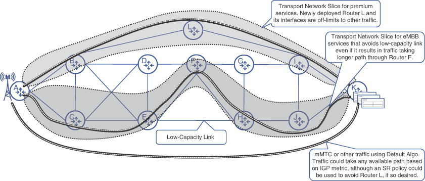
FIGURE 6-14 Network Slices in an MCN
While Flex-Algo plays a critical role in implementing transport network slicing, its ability to optimize the number of SIDs for a given constrained path makes Flex-Algo an effective network-scaling mechanism. As mentioned earlier, a constrained path might require multiple SIDs to be stacked on top of the packet, thereby increasing the packet size as well as introducing the risk that some devices might not have the hardware capability to impose or parse the excessively large SID list. While a mechanism such as MSD propagation is used as a preventive measure, it does not offer a solution to lower the numbers of SIDs in the packet. Flex-Algo, on the other hand, not only provides a slicing mechanism, but it can also reduce the number of SIDs required to forward traffic along a constrained path.
Because Flex-Algo fundamentally alters the metric used to calculate a path, the next hop (or rather the SID associated with the next hop within the Flex-Algo domain) becomes an instruction to reach that waypoint using the metric associated with the FAD. For instance, if a Flex-Algo uses delay as the metric, then the SID for the destination would represent the best path using the lowest delay, instead of the lowest link cost. This is in contrast to the default algo, where if the lowest delay path were to be used, the headend would need to impose multiple SIDs, representative of the lowest latency path, should that path be different from the cost-based path. In essence, Flex-Algo not only makes it easier and efficient to implement transport network slicing, it inherently optimizes and reduces the number of SIDs a headend may need to impose on the packet, as shown in Figure 6-15. Due to its rich feature set and effectiveness, Flex-Algo is also listed as both a transport-slicing and network-scaling mechanism in O-RAN’s xHaul Packet Switched Architecture Specification.
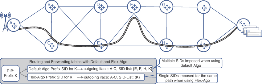
FIGURE 6-15 Lowering SID List with Flex-Algo
Redundancy and High Availability with Segment Routing
Besides achieving the primary objectives of efficient network utilization and custom forwarding paths for certain traffic types, MPLS-TE was instrumental in another aspect of network operation—rapid restoration of traffic forwarding. Thanks to its fast reroute (FRR) capabilities, MPLS-TE offered various types of path protection, typically restoring traffic forwarding within 50ms upon failure detection.36 In fact, MPLS-TE FRR became so popular that many networks deployed MPLS-TE for the sole intention of using its FRR feature.
MPLS-TE FRR features were followed by IP Fast Reroute (IP-FRR), also known as Loop-Free Alternates (LFA).37 Being an IP-only feature, LFA offered a path-protection mechanism that does not require an MPLS forwarding plane for detours. LFA leverages the IGP’s SPF algorithm to pre-calculate backup paths toward destinations, while considering a failure in the directly connected links or nodes that are used as the primary path to those destinations. For all destinations, the FIB is programmed with a pre-computed backup path, which takes over immediately upon detection of a failure on the primary link, thus reducing convergence times.
While LFA is a very effective and simple-to-use mechanism for path protection in IP-only networks, it has a major drawback. LFA is topology dependent and, in some networks, it cannot offer any backup paths to protect traffic. If paired with LDP, it can further be extended to such topologies and is called Remote LFA or rLFA. Using rLFA, a backup path in the form of MPLS LSP is established to remote nodes, thus providing FRR capabilities to scenarios where IP-only LFA is not possible.
Segment Routing offers a new Topology-Independent Loop-Free Alternate (TI-LFA) path-protection mechanism by extending LFA and rLFA principles to use Prefix- and Adjacency-SIDs for effective and topology-independent restoration of a traffic path after link or node failures.38
Segment Routing Topology Independent Loop-Free Alternate
The TI-LFA mechanism is based on the same theory as LFA and rLFA, but applied to an SR-enabled network. Similar to its predecessors, the feature is local to the node and can provide rapid traffic path restoration for local adjacency failure scenarios. No additional information, besides what is already known in the SR-enabled network, is needed for TI-LFA operation. The core of the TI-LFA algorithm is the analysis of what-if scenarios, where a primary adjacency, used as an outgoing link for a given destination, fails. The analysis results in a pre-calculated backup path being installed for each destination into the FIB. This backup path must use a different outgoing interface, compared to the primary path, and may involve a few SIDs added on top of the packet to enforce the desired backup path.
Depending on the configuration, TI-LFA can treat the failure of an adjacency as a link or a node failure. In the latter case, the backup path is calculated to avoid the whole node rather than just the link. If no suitable backup paths are found for node protection, the routers may fall back to link-protection calculations.
Although TI-LFA is called “topology independent,” strictly speaking it still depends on the topology because at least one alternate path should exist. Moreover, the SID-list, calculated by TI-LFA for a destination prefix, also depends on the topology. This SID-list may be composed of multiple SIDs to force traffic over certain links in the network regardless of their metric, or may be empty. As shown in Figure 6-16, node B’s primary path toward K goes via nodes C, E, H, and J. If the adjacency with C fails, node B simply switches the outgoing interface to the adjacency with node D. No additional SIDs are required to enforce a loop-free backup path toward K. Conversely, besides switching the outgoing interface, the backup path from node C toward prefix K requires pushing two SIDs: the Prefix-SID of node B and the Adjacency-SID of B’s adjacency to node D. This is due to the high metric on the link between nodes B and D. Without this SID-list, node B will try to forward packets with Prefix-SID K back to node C, causing a loop.

FIGURE 6-16 TI-LFA Backup Paths Example
When enabled, the TI-LFA algorithm is executed by the IGP for each destination as soon as that destination is learned. If a loop-free alternate is found for the destination, the appropriate SID-list and outgoing interface is installed in the FIB as a backup path for the destination. With the pre-computed backup path installed, the decision to switch over is made by the FIB without waiting for IGP to reconverge. Upon detection of an adjacency failure, all destinations using this adjacency as a primary outgoing interface immediately switch over to their respective backup paths, which remain active until the network reconverges.
As in the case of MPLS-TE FRR or IP-LFA, the failure detection is critical to any rapid restoration mechanism. Just enabling TI-LFA may not achieve the goal of recovering from a failure within 50ms without suitable failure detection. Normally, link failures are detected by the loss of signal on the receive side of the interface transceiver. In this ideal failure-detection scenario, the detection is instantaneous and restoration of traffic forwarding, by switching to a backup path in the FIB, is almost immediate and can easily meet the 50ms target. However, if the link to another node is transported by some other device (for example, WDM transport), the fiber cut might not necessarily result in the loss of signal on the router’s interface. In the absence of other detection mechanisms, the router would need to wait until IGP declares the link as down, which may take a few dozen seconds with default IGP timers. To avoid such scenarios, many network architects prefer to use the Bidirectional Forwarding Detection (BFD) mechanism, ensuring detection of link failures within just a few milliseconds.
Segment Routing Loop Avoidance Mechanism
TI-LFA rapid restoration acts quickly to repair a broken path, but in doing so it may use a non-optimal path toward the destination. After IGP converges over the new topology, the router updates primary paths toward impacted destination prefixes, recalculates backup paths, and, if SR-TE is used, re-optimizes the SR policy path.
TI-LFA is effective in reacting to local adjacency failures and, if enabled on all nodes in the network, delivers a reliable rapid restoration method. Nevertheless, link failures or sometimes even link-up events might cause short-lived or transient loops in the network. As shown in Figure 6-17, a new link between nodes F and H comes up with a metric of 5 and node B’s IGP receives and processes the topology change information before node D does. Due to the high metric between nodes G and I, node D might still consider B as a best next hop to reach K. Yet, node B already knows that the best path to K is via D, F, H, and J. This results in a microloop between B and D for a short period of time.
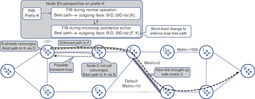
FIGURE 6-17 Loop-Avoidance Mechanism
The mechanism to avoid transient loops is proposed in the IETF draft Loop Avoidance Using Segment Routing and is already implemented as the SR microloop avoidance feature by multiple vendors.39 Using the example from Figure 6-17, the loop-avoidance mechanism alters node B’s behavior. In order to avoid packets from looping between B and D, node B enforces traffic to be safely delivered to node F, by pushing Prefix-SID of F on top of the packet, justifiably assuming F’s IGP has already converged. This enforced path remains in effect for a preconfigurable duration and then removed from the FIB, reverting back to normal forwarding.
The loop-avoidance mechanism is triggered by IGP upon receiving remote or direct link-down or -up events and uses a timer-based approach to keep loop-mitigating path enforcement in place. This mechanism is not intended to replace TI-LFA but rather complement it.
Segment Routing for IPv6 (SRv6)
Although current deployments of Segment Routing are predominantly SR-MPLS, where labels are used as a representation of SIDs, an alternate approach is starting to emerge for IPv6-enabled networks. Instead of relying on the MPLS forwarding plane, Segment Routing can use the IPv6 forwarding plane almost natively, thanks to IPv6’s enormous address space and extensible headers. Technically speaking, source routing capabilities were part of the IPv6 standard a long time before Segment Routing was introduced. Extension headers could include the routing header, which lists a set of IPv6 addresses for a packet to visit. What is different in Segment Routing v6 (SRv6), however, is how IPv6 addresses are used both in the destination address of an SRv6 packet and in the routing extension header. This section expands on the SRv6 implementation in an IPv6 network.
IPv6 Adoption and Challenges
SRv6 requires an IPv6 forwarding plane, be it dual-stack (IPv4 and IPv6) or native IPv6 network. Although the promise of transitioning the networking world from IPv4 toward a future-proof IPv6 address space remains unfulfilled after more than two decades, the strides to get broader IPv6 adoption have resulted in more than 35% of users accessing the Internet using IPv6 natively today.40 Significant challenges, such as a lack of capable customer premises equipment (CPE) to support IPv6, complex migration paths, massive software and hardware upgrades, and outright inertia, to name a few, have slowed down this trend over the preceding years. In the wake of these challenges, innovative mechanisms, such as Carrier-Grade Network Address Translation (CGNAT), allowed many service providers to stay in the IPv4 comfort zone. Some say that IPv6 lacks a killer application to push for a fast transition and, although debatable, there is a possibility that by selecting SRv6 as one of the 5G technology enablers, the O-RAN Alliance might have just made SRv6 a killer app for the industry’s transition to IPv6.
Segment Information as IPv6 Address
The fundamentals of Segment Routing implementation for the IPv6 network (SRv6) do not differ from SR-MPLS (that is, the concept of segments, the use of SIDs, and the use of IGP by the control plane to propagate SID information across the network). Instead of using MPLS labels as SIDs, as was done for IPv4 networks, SRv6 repurposes the 128-bit Destination Address (DA) field in the IPv6 header.
Just like in SR-MPLS, the SRv6 SID identifies an instruction on a particular node. For SRv6, this instruction is advertised as a single 128-bit value that can be logically split into two parts. The first group of bits, called Locator, uniquely identifies the node, while the remaining bits, called Function, are used to define special traffic treatment upon reaching the node. Depending on the Function, the SID can represent a Node-SID, Adjacency-SID, or other types of SIDs. Thus, the Functions here are analogous to SID types in SR-MPLS. A node may define multiple such SID values, each with a different Function. Figure 6-18 shows the use of the DA field in an IPv6 header for an SRv6 SID.

FIGURE 6-18 Repurposing IPv6 Header’s DA for SRv6 SID
These SIDs can then be advertised to the IPv6 network using newly defined IGP TLVs for SRv6.41 The SRv6-capable routers in the network will interpret the TLVs and build their information table for advertised SIDs, while installing the appropriate entries in their forwarding table. Additionally, the Locator portion of the SIDs is advertised as an IPv6 prefix. It allows for any non-SRv6-capable router in the network to learn the Locator like any other IPv6 prefix, while ignoring the SRv6 TLVs. The SRv6-capable routers can now send traffic toward any of these SIDs by simply using that SID as a destination address in the IPv6 packet, letting the packet take the best IGP path. This simple idea of using IPv6 predefined fields was further extended for SR-TE capability in SRv6. The SID list is computed using the constraint-based SPF calculations (just like in case of SR-MPLS), either locally at the headend router or by the PCE. This SID-list is then embedded into the IPv6 Header. If this list comprises more than one SID, then a newly defined IPv6 routing extension header called Segment Routing Header (SRH) is used to embed this list into the IPv6 header.42 The SRH uses a predefined option in IPv6 to add a header field called routing header. The type field of the routing header is set to type 4, indicating the header will be used for SIDs. SRH then stores the SID-list in the type-specific data field of the routing header.
The first SID from the list is also copied to the DA field of the IPv6 header, and standard IPv6 routing and forwarding take care of the rest. That destination router recognizes the presence of SRH, copies over the next SID from the SRH as a new destination address, and decrements the Segments-Left field in the SRH. It then proceeds to forward the packet to the new destination. The process will be repeated, until the Segments-Left counts down to 0, at which point the SRH is removed and the last SID is copied over to the DA. This process is called Penultimate Segment Pop (PSP). The packet then gets routed toward the DA, which was effectively the last SID in the list. This results in the flow of data through the exact engineered path that was determined at the headend node. Figure 6-19 shows this process as the packet traverses the network.
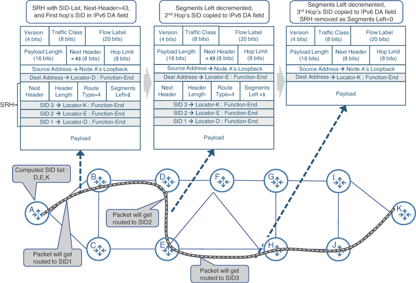
FIGURE 6-19 Traffic Engineering with SRv6
Despite its simplicity, the use of SRH for SR-TE experienced some headwinds for real-world implementations. The SRH with the list of 128-bit SIDs bloats up the IPv6 header, thus adding significant overhead. Additionally, the imposition of this stack at the headend and the processing of it at the intermediate nodes are resource heavy for the forwarding CPU. More recently, to overcome and avoid these potential inefficiencies, a few new approaches have been proposed. These ideas revolve around recognizing that using the entire 128-bit space is overkill for a single SID value and instead suggest using shorter SID values. This offers more efficient use of the IPv6 header space, and either significantly reduces the need for SRH or makes SRH compact. With these implementations, the SRv6 routers will now need to use special manipulation on the DA field, instead of replacing it with a new SID from the list. There are multiple competing IETF drafts that are currently under discussion and making their way through the standardization process. Two current front-runners that suggest shorter SRv6 SIDs are SRv6 micro-segment (uSID) and Segment Routing Mapped to IPv6 (SRm6).43,44
Segment Instructions in SRv6
As mentioned earlier, an SRv6 SID consists of a locator and a function. Each of these functions defines a certain instruction to be executed upon reaching the Locator node. These instructions are called behaviors in SRv6 specification, and an SRv6-capable node should support some, if not all, of these. This section details some of the primary behaviors performed by the SRv6 forwarding plane.
Headend Encapsulation (H.Encaps) is a behavior implemented by SRv6 headend when it steers a packet into SRv6 policy. This behavior can be compared to an MPLS label push operation, when a stack of labels expressing a SID-list is added on top of the packet. Instead of a label stack, SRv6 pushes another IPv6 header and installs SRv6 SID into the Destination Address (DA) field of the packet. In its current implementation, when the SRv6 SID-list contains more than one SID, an SRH is added to the packet. H.Encaps can be optimized by one of the emerging SRv6 drafts discussed earlier.
The same behavior can be applied to L2 frames, for example, while using L2VPN service, in which case it is called H.Encaps.L2. The entire frame can be encapsulated into an IPv6 packet following the same logic, by putting the SRv6 SID into the DA field and the possible addition of SRH.
H.Encaps.Red and H.Encaps.L2.Red are flavors of H.Encaps and H.Encaps.L2, respectively, with a simple difference: these behaviors do not include the first SRv6 SID, already installed in the DA field, in their SRH. This reduces the SRH size and hence the name of the behavior.
The MPLS label-swap operation equivalent is not specifically called out in the standard. For any non-end-of-segment node, it is simply usual forwarding operation based on the DA field. Interestingly enough, this means that any IPv6-enabled router can forward SRv6 packets, even if it does not explicitly support SRv6. Of course, such a router cannot be an SRv6 headend or endpoint or otherwise act as an end-of-segment node.
The End behavior in SRv6 can be mapped to the MPLS label pop operation, whereupon reaching the end of the segment, the active SID should be removed from the packet. The SRv6 endpoint implements this operation by replacing the SRv6 in the DA field by the next SID from the SRH. When there is no SRH or no active segment in the SRH, the endpoint should pop the current IPv6 header and start processing the next header. The basic End behavior in SRv6 can be seen as an equivalent of a Prefix-SID. Besides this basic End behavior, there are many other, more specialized flavors of the End behavior defined in the standard to implement a rich set of instructions supported by SRv6, a few of which are covered in this section.
End.X behavior is a flavor of End SRv6 behavior. The X in its name stands for the L3 Cross-Connect action, and this behavior is an equivalent of an Adjacency-SID in SR-MPLS. Besides replacing the DA field in the SRv6 packet, or removing the header and SRH altogether, the SRv6 node forwards the packet over a specific L3 adjacency, without any further processing or lookups.
End.DX4 and End.DX6 behaviors instruct a router to decapsulate a packet and cross-connect it with IPv4 or IPv6 adjacency, respectively. It pops the IPv6 header and exposes the underlying IPv4 or IPv6 packet, which is then forwarded over a specific IPv4 or IPv6 adjacency without additional lookup. These behaviors can be considered as an equivalent of a per-CE L3VPN label paired with a transport label for the advertising PE. Indeed, the locator part of the SRv6 SID helps to bring the packet to the correct PE, while the function part of the SRv6 SID identifies which VRF to use.
End.DT4 and End.DT6 behaviors are very similar to the previously described End.DX4 and End.DX6, with one significant difference. These behaviors instruct the router to execute a lookup on the exposed packet in the appropriate table. The direct equivalent of using these behaviors would be L3VPN with per-VRF label allocation.
End.DX2 is another flavor of an End behavior, applicable to L2 Ethernet frames. The End.DX2 behavior is typically associated with L2VPN or EVPN services, but otherwise works similarly to the End.DX4 and End.DX6 behaviors.
Note
End behaviors, like other SRv6 components, may evolve with the development of existing and new SRv6 specifications.
Many other types of End behaviors are already defined in the IETF “Segment Routing over IPv6 (SRv6) Network Programming” standard; however, this list is likely to grow over time.45
Implementing Services with SRv6
A few characteristic features of SRv6 make it an attractive option for network architects. First off, it is ultra-scalable. With 128 bits available for SRv6 locators and functions, it is hard to imagine a network exhausting this enormous space. SRv6 can easily support a typical MCN deployment with its vast number of cell site routers and numerous domains, without the need of a Seamless-MPLS-type workaround.
Secondly, SRv6 runs natively on the IPv6 forwarding plane and can even leverage non-SRv6 routers running vanilla IPv6 along the path of an SRv6 policy. For an IPv6-enabled network, the use of SRv6 may eliminate the need to keep special MPLS tables, freeing up NPU’s precious on-die memory resources. The ability to incorporate information about the VPN itself and reachability to the PE in a single SRv6 SID provides an efficient way to deploy services with SRv6. The same functionality requires multiple labels in an SR-MPLS environment.
While SRv6 is starting to gain popularity, it should not be a surprise that at the time of this writing, SR-MPLS is the technology of choice for Segment Routing deployments. The transition from MPLS-LDP to SR-MPLS is greatly facilitated by the ability of SR-MPLS to run in parallel with existing label distribution protocols. SRv6, on the other hand, requires end-to-end IPv6, yet the level of IPv6 adoption in today’s networks falls behind the ubiquitous MPLS in the SP and enterprise world. Nevertheless, SRv6 is considered a pathway forward in mobile communication networks, whereas SR-MPLS is here today.
Summary
This chapter took a deep dive into the fundamentals of Segment Routing, an emerging transport network technology that is fast becoming a de facto standard for any 5G-ready mobile transport network.
This chapter discussed the following topics:
Evolution of the MPLS-based networks through the use of purpose-built protocols and resulting operational complexities
Fundamentals of Segment Routing and various types of segment IDs
Segment Routing Traffic Engineering and its role in programming a traffic path through the network using Constraint-based Shortest Path First algorithms
Mechanisms of traffic steering into SR policies
Building blocks of a software-defined transport
Use of PCE as a transport SDN controller and its interaction with the network and higher-layer applications
5G transport network slicing with SR Flexible Algorithms
Rapid restoration and loop-avoidance mechanisms used by Segment Routing
An introduction to Segment Routing on the IPv6 network (SRv6)
Chapter 7, “Essential Technologies for 5G-Ready Networks: DC Architecture and Edge Computing,” will focus on data centers, which is another critical technology to build 5G networks. The chapter will discuss design principles of these DCs and their integration with SR-enabled xHaul networks.
References
1. “World’s Largest LTE Deployment—Reliance JIO India,” https://www.ciscolive.com/c/dam/r/ciscolive/us/docs/2017/pdf/CCSSPM-1004.pdf, slide 20 (last visited: July 2021)
2. IETF RFC 8402, “Segment Routing Architecture”
3. Ibid.
4. Ibid.
5. IETF RFC 8986. “Segment Routing over IPv6 (SRv6) Network Programming”
6. IETF RFC 8402, op. cit.
7. IETF RFC 8669, “Segment Routing Prefix Segment Identifier Extensions for BGP”
8. “BGP-LS Extensions for Segment Routing BGP Egress Peer Engineering” (IETF draft), https://datatracker.ietf.org/doc/html/draft-ietf-idr-bgpls-segment-routing-epe-19 (last visited: July 2021)
9. IETF RFC 8402, op. cit.
10. IETF RFC 8667, “IS-IS Extensions for Segment Routing”
11. IETF RFC 8665, “OSPF Extensions for Segment Routing”
12. IETF RFC 8666, “OSPFv3 Extensions for Segment Routing”
13. IETF RFC 8669, op. cit.
14. IETF RFC 3209, “RSVP-TE: Extensions to RSVP for LSP Tunnels”
15. “Segment Routing Policy Architecture” (IETF draft), https://datatracker.ietf.org/doc/html/draft-ietf-spring-segment-routing-policy (last visited: Mar 2022)
16. Ibid.
17. Ibid.
18. “Advertising Segment Routing Policies in BGP” (IETF draft), https://datatracker.ietf.org/doc/html/draft-ietf-idr-segment-routing-te-policy/
19. Ibid.
20. IETF RFC 4655, “A Path Computation Element (PCE)-Based Architecture”
21. RFC 5440, “Path Computation Element (PCE) Communication Protocol (PCEP)”
22. IETF RFC 7752, “North-Bound Distribution of Link-State and Traffic Engineering (TE) Information Using BGP”
23. RFC 5440, op. cit.
24. “Advertising Segment Routing Policies in BGP,” op. cit.
25. “Northstar Controller,” https://www.juniper.net/content/dam/www/assets/datasheets/us/en/network-automation/northstar-controller.pdf
26. https://www.cisco.com/c/en/us/td/docs/cloud-systems-management/crosswork-infrastructure/4-0/InstallGuide/b_cisco_crosswork_platform_40_and_applications_install_guide/m_overview.html (last visited: Feb 2022)
27. 3GPP TS 28.530 version 15.0.0, Release 15, “5G; Management and orchestration; Concepts, use cases and requirements,” https://www.3gpp.org/
28. O-RAN xHaul Packet Switched Architectures and Solutions, https://www.o-ran.org/specifications
29. Ibid.
30. “IGP Flexible Algorithm” (IETF draft), https://datatracker.ietf.org/doc/html/draft-ietf-lsr-flex-algo (last visited: Feb 2022)
31. IETF RFC 8570, “IS-IS Traffic Engineering (TE) Metric Extensions”
32. IETF RFC 7471, “OSPF Traffic Engineering (TE) Metric Extensions”
33. “BGP-LS Advertisement of IGP Traffic Engineering Performance Metric Extensions” (IETF draft), https://datatracker.ietf.org/doc/html/draft-ietf-idr-te-pm-bgp (last visited: Feb 2022)
34. IETF RFC 5357, “A Two-Way Active Measurement Protocol (TWAMP)”
35. IETF RFC 6374, “Packet Loss and Delay Measurement for MPLS Networks”
36. IETF RFC 4090, “Fast Reroute Extensions to RSVP-TE for LSP Tunnels”
37. IETF RFC 5286, “Basic Specification for IP Fast Reroute: Loop-Free Alternates”
38. “Topology Independent Fast Reroute Using Segment Routing” (IETF draft), https://datatracker.ietf.org/doc/html/draft-ietf-rtgwg-segment-routing-ti-lfa (last visited: Feb 2022)
39. “Loop Avoidance Using Segment Routing” (IEFT draft), https://datatracker.ietf.org/doc/html/draft-bashandy-rtgwg-segment-routing-uloop/ (last visited: Feb 2022)
40. IPv6 usage statistics, https://www.google.com/intl/en/ipv6/statistics.html
41. “IS-IS Extensions to Support Segment Routing over IPv6 Dataplane,” (IEFT draft), https://datatracker.ietf.org/doc/html/draft-ietf-lsr-isis-srv6-extensions (last visited: Feb 2022)
42. REF2: IETF RFC8754, “IPv6 Segment Routing Header (SRH)”
43. “Network Programming extension: SRv6 uSID instruction” (IETF draft), https://datatracker.ietf.org/doc/draft-filsfils-spring-net-pgm-extension-srv6-usid (last visited: Feb 2022)
44. “Segment Routing Mapped to IPv6 (SRm6)” (IETF draft), https://datatracker.ietf.org/doc/html/draft-bonica-spring-sr-mapped-six (last visited: Feb 2022)
45. Ibid.