Chapter 2
Anatomy of Mobile Communication Networks
Various individual components and interconnected systems come together to make an end-to-end mobile communication network (MCN). The previous chapter introduced the evolution of mobile generations in the context of three distinct MCN domains, namely:
Radio access networks (RANs): These networks comprise discrete interconnected components that collectively provide the air interface to connect the end user of the mobile services to the mobile network.
Mobile transport and backhaul: The network infrastructure that provides connectivity between RANs and the mobile core.
Mobile core: The brain of an MCN. The mobile core enables and implements services for the end users.
Mobile services rely on each of these domains working together in cohesion. A deeper understanding of the anatomy of these domains, as well as the interaction within and between them, is critical for designing effective mobile network architectures. This chapter will take a closer look at these distinct yet tightly interconnected domains that make up an end-to-end mobile communication network.
Understanding Radio Access Network
The RAN is perhaps the most prominent component of the mobile communication network. It is also the interface between a mobile operator and its subscriber. A vast majority of mobiles users remain completely oblivious to the rest of the network’s components, typically equating the quality of their overall service to an operator’s RAN performance. Mobile operators obviously seem to be aware of this and use slogans like “Can you hear me now?” (Verizon) or “More bars in more places” (AT&T)—a nod to the performance and reliability of their RAN—in an effort to win market share.
While the perceived key measure of RAN performance is cellular coverage, there are actually many factors that contribute to an efficient RAN design. Mobile operators spend a lot of effort, time, and money ensuring optimal operations and continued RAN enhancements. Although radio frequency (RF) planning and optimization might be an apt topic for a book on its own, this section provides a brief overview of key RAN concepts.
Units of Radio Frequency
When Heinrich Hertz proved the existence of electromagnetic waves through his experiments between 1886 and 1889, nobody, including Hertz, believed that there could be any real-life applications for them. Initially referred to as Hertzian waves and later commonly called radio waves, these electromagnetic waves were measured in cycles per second (CPS). The cycles represent the frequency of oscillations per second, with higher frequency waves being measured in kilo-cycles (kc) and megacycles (mc). As an honor to Heinrich Hertz, cycles per second was replaced with Hertz (Hz) as the unit of frequency measurement in 1920 and was officially adopted by the International System of Units in 1933.
How the RF Spectrum Is Allocated
When electromagnetic waves propagate, they don’t directly affect each other. Yet, a receiver detects the superposition of electromagnetic waves as they appear in certain points in space. This phenomenon, called interference, restricts the receiver’s ability to reliably detect radio waves emitted by a specific transmitter. When two transmitters, in close proximity to each other, emit radio waves in the same direction and at the same frequency, it is very hard or sometimes impossible to detect individual transmission. To avoid this scenario, the concept of “right to use” was introduced to regulate the use of radio frequencies within a geographical area.
As part of the right-to-use process, the “usable” frequency ranges would first be defined by the standard bodies. Based on these standards, the regulatory bodies (that is, government agencies) would then auction off the rights to use these frequencies within a geographical area to various operators. New frequency ranges are sometimes made available, either due to technological enhancements or through the repurposing of a previously allocated spectrum, kicking off a new round of auctions. The right is to a frequency range in a particular market is a valuable commodity, one which mobile operators spend hundreds of millions, if not billions, of dollars to acquire and use. One such example is FCC Auction 107, where a mere 280MHz spectrum attracted bids upward of $80 billion.1
Mobile operators are not the only users of the radio frequency spectrum. Public services (law enforcement, fire departments, first responders, hospitals), broadcasting (radio and television), as well as government and military services are all consumers of the radio spectrum. As such, government bodies tasked with regulating the RF spectrum set aside various frequency ranges for specialized use. For instance, in the United States, radio frequencies in the 535–1705KHz range are reserved for AM radio broadcast, 88–108MHz are reserved for FM radio, and 54–72MHz, 76–88MHz, 174–216MHz, and 512–608MHz are reserved for TV broadcast.2, 3
In addition to auctioning off frequency ranges for exclusive use of mobile operators, some frequency ranges are made available to operators for unlicensed usage. One such example is the Citizens Broadcast Radio Service (CBRS) in the U.S. CBRS and its equivalent around the world, such as Licensed Shared Access (LSA) in Europe, provide specific frequency spectrum ranges to new and incumbent mobile providers as well as to private entities for various uses, including deploying mobile networks. This is done, in part, to foster competition and to lower the cost of entry for startups. CBRS and other free-to-use spectrums are an important part of mobile standards.
Choosing the Right Frequency
Radio waves operating at different frequencies have different characteristics in terms of their applicability for mobile services. For instance, radio waves in lower frequency ranges are less susceptible to absorption and reflection by obstacles. These radio waves tend to bend easily around corners, a phenomenon called diffraction, and would therefore penetrate buildings and structures better, thus providing superior signal propagation. Conversely, higher frequency radio waves tend to be more susceptible to obstacles and have far worse penetration within buildings and structures.
Another factor affecting radio transmission is the way antennas emit and receive radio waves. Although many different antenna types exist and are used for different purposes, mobile communication systems usually rely on omnidirectional antennas in their mobile devices. The size of a typical omnidirectional antenna is a function of its operational frequency and becomes proportionally smaller for higher frequencies. This has a profound effect on the reception of radio waves by omnidirectional antennas. Due to its smaller effective area, a high-frequency omnidirectional antenna collects less energy compared to its lower-frequency counterpart at the same distance from the transmitter. In other words, smaller high-frequency omnidirectional antennas produce weaker electrical signals at the inputs of a receiver. Hence, this effectively reduces the usable distance of a higher-frequency transmission even in the absence of obstacles. This dependency is routinely included in the equations used by radio engineers designing transmission systems and is often referred to as free space path loss. Despite its utility in radio engineering, the free space path loss equation and concepts can be somewhat misleading, as this effect is not inherent to higher-frequency radio waves themselves and is rather caused by the omnidirectional antennas’ operational principles. High-frequency radio transmissions can be successfully implemented over great distances with the use of directional antennas (for example, dish antennas). Mobile devices, however, are typically designed with omnidirectional antennas for better usability, but there are trade-offs in terms of effective coverage area for higher-frequency bands.
If signal propagation was the only goal, a provider would use lower-frequency ranges in locations with more buildings and structures such as a metro downtown. In that case, higher-frequency ranges would then be reserved for suburbs and open spaces such as along stretches of highways. Signal propagation is just one of the factors in a provider’s RF strategy, however. There are other factors to consider as well, such as the width of the frequency range.
The radio frequency range, known as a frequency band, is akin to highway traffic lanes. The wider the highway, the more individual traffic lanes that can be fit in either direction. The more traffic lanes there are, the more cars that can simultaneously use the highway. The same is true of radio waves and mobile traffic. The individual highway lanes are the “channels” in a mobile radio network that carry mobile traffic. An individual channel, also called carrier channel, is a range of frequencies within the available spectrum. Generally speaking, the channel width and the total number of channels in a defined frequency spectrum determine overall traffic capacity.
Simply put, a frequency band is a range of frequencies, and a carrier channel is a subset of a frequency band used for mobile communications. Channels are characterized by their width and central frequency, also called the carrier frequency. In mobile communications, it is the carrier frequency that is then modulated to produce the resulting signal.
Each mobile generation has defined the carrier channel width as well as the supported frequency spectrum. For instance, 1G AMPS networks used a channel width of 30KHz, while their European counterpart, ETACS, used 25KHz channels. AMPS used frequency bands in the range of 824–849MHz for user-to-base-station communication (referred to as reverse link in the mobile world and upstream frequency from a network’s perspective) and 869–894MHz for base-station-to-user communication (referred to as forward link or downstream frequency). ETACS had defined 890–915MHz as upstream and 935–960MHz as downstream frequency bands. With defined channel widths of 30KHz and 25KHz, AMPS and ETACS allowed for 832 and 1000 channels, respectively, in each direction.
Correlating Frequency Ranges and Capacity
Recent advances in electronics have unlocked the use of higher frequency ranges (24GHz and higher). These higher frequency ranges have wider bands available, providing the capability for not only more channels but also wider channel widths. For instance, between 900 and 910MHz, there is 10MHz or 10,000,000Hz available, whereas between 2.4 and 2.5GHz, there is 100MHz available that can be utilized for various channels. Hence, it should be kept in mind that when frequencies are listed in GHz, a small delta in the numbers would reflect a large step when compared to MHz. This is a subtle distinction that is easy to overlook.
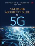
Newer generations introduced higher channel widths (for example, 200KHz for GSM, 5MHz for most 3G implementations) as well as new frequency ranges. 1G and 2G networks primarily used the frequencies below 1GHz, whereas 3G and 4G defined and used additional higher-frequency ranges between 1 and 6GHz. Recently, 3GPP Release 16 extended this range to 7.125GHz. Today, the frequencies below 1GHz (also called sub-1GHz frequencies) are referred to as low-band, whereas the frequencies in the 1–7.125GHz range (also called sub-7GHz frequencies) are called mid-band frequencies. These low-band and mid-band frequency ranges are collectively referred to as Frequency Range 1 (FR1).
More recently, the use of frequencies higher than 24GHz has been defined for mobile communication as well. These frequencies are classified as high-band frequencies and referred to as Frequency Range 2 (FR2). These ultra-high frequencies are also called millimeter wave (mmWave) frequencies, due to their wavelengths being a few millimeters. Figure 2-1 shows various frequency band classifications, their relative spectrum availability, and their propagation efficiency characteristics.

FIGURE 2-1 Frequency Band Classifications
Going back to the analogy of highway traffic lanes, larger frequency bands represent highways that can now fit more and wider traffic lanes, thus providing higher capacity. From a transport network perspective, the use of higher-frequency ranges, where wider channels are more readily available, results in greater overall bandwidth requirements to adequately support all services.
The frequency range used by a provider is dependent on three primary factors:
Whether the frequency range has been introduced for use by standard bodies such as 3GPP
Whether the regulatory authorities have made the frequency spectrum available
Whether the provider has the rights to use that particular frequency band for a given geographical area
As long as the preceding three criteria are met, a provider could use a frequency range for their 2G, 3G, 4G, or 5G service offerings. Frequency spectrum is not tied to a single generation, and a provider may repurpose a previously used band, assigning it for a newer generation of mobile service. In reality, low-band frequencies that have been available since 1G and 2G networks were the first ones to be repurposed and used in 5G networks. Figure 2-2 illustrates this frequency use and reuse across generations.
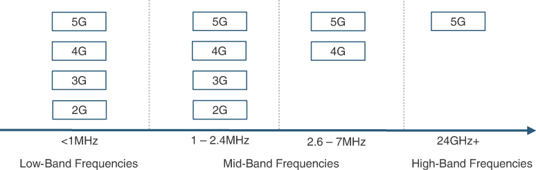
FIGURE 2-2 Typical Frequency Band Usage Across Mobile Generations
To summarize, frequencies in low bands have better propagation efficiency than higher ones, while mid and high bands offer more and wider available channels, which translates into higher overall system capacity. Using high bands might require direct line of sight or close proximity to the radio tower to provide adequate coverage. In that context, mid-band frequencies (below 7GHz) provide a good balance of coverage and capacity, and hence attract extremely high bids for acquiring right of use.4 The highly sought-after C-Band frequencies fall under this category. For example, in the year 2021 Verizon Wireless spent about $53 billion to acquire an average of 161MHz of C-Band spectrum for nationwide use in the USA. C-Band spectrum is the higher end of mid-band frequencies (that is, above 3GHz) which has been allocated for cellular use.
Mobile operators typically use a mix of various frequency bands. Due to their propagation properties, low-frequency bands are often better suited for suburban and rural areas, whereas higher bands might be preferred in dense urban areas. In reality, multiple frequency bands are used within the same cell to provide a mix of coverage and speed to as many mobile users as possible.
RF Duplexing Mechanisms
All radio transmissions are simplex (that is, unidirectional) in nature. This means that for the mobile phone and antenna on the cellular tower to communicate in both directions, duplexing techniques are required. The two primary techniques used to achieve duplex communication in mobile systems are Frequency Division Duplex (FDD) and Time Division Duplex (TDD).
FDD uses two separate frequencies for uplink and downlink communications. In this case, both the mobile phone and cell tower would transmit and receive at the same time, albeit on different frequencies. When an FDD schema is used, the uplink and downlink frequency bands are separated by what is called a guard band. This guard band is an unused frequency channel that provides a buffer between the uplink and downlink channels to minimize interference between the two. An example of an FDD guard band would be the 20MHz channel between the 1850–1910MHz uplink and 1930–1990MHz downlink frequencies specified for operating band number 2.5
Operating Band Numbers
Supported frequency ranges are typically identified by a band number and a common name. There is no direct correlation between a band number and its frequency range, as the ranges are added as and when it becomes feasible to do so. Hence, band 1 (commonly called 2100) defines 1920–1980MHz for upstream and 2110–2170MHz for downstream, while band 2 (called PCS 1900) identifies 1850–1910MHz and 1930–1990MHz. The specification also defines if an operating band uses FDD or TDD as the duplexing mechanism.
In 5G specifications, the previously defined band numbers are prefixed with n (for example, band 1 becomes n1) and new operating bands are specified as well. Before 5G, a total of 88 operating bands were defined.6 5G NR Base Station (BS) radio transmission and reception specification by 3GPP currently specifies operating bands n1 though n96 in the FR1 frequencies and addition band in FR2 frequency ranges.7
TDD is another mechanism used to provide duplex communications between a cell tower and mobile equipment. In TDD, a single frequency is used in both upstream and downstream directions, but it uses different timeslots to achieve duplex communication. With this approach, there is no need for a guard band; however, the timeslots are now separated by a guard interval that ensures transmit and receive timeslots do not overlap. The guard interval should be long enough to accommodate for signal propagation time between transmitter and receiver. The use of a guard interval introduces inefficiencies in spectral usage, as no signal transmission can occur for the duration of the guard interval. Likewise, inefficiencies also exist in FDD transmission in cases where a frequency band is left unused in order to provide the guard band function. Figure 2-3 provides an overview of TDD and FDD mechanisms in mobile systems.

FIGURE 2-3 TDD and FDD Duplexing Mechanisms
There are pros and cons to both duplexing techniques. FDD has been in use since the early days of mobile communications, making it a proven and more widely deployed technology. With dedicated upstream and downstream frequencies, FDD offers traffic symmetry and continuous communications in either direction. On the other hand, FDD contributes to spectral wastage due to the need of allocating frequencies in pairs and setting aside a guard band to separate upstream and downstream frequencies. The hardware costs for FDD-based systems are typically higher than their TDD counterparts due to the use of diplexers—passive devices to separate upstream and downstream bands using frequency-based filtering.
TDD systems adjust well to asymmetrical traffic distribution, as is typically the case with consumer data traffic. With timeslots allocated for transmit and receive over the same frequency band, it is possible to adjust timeslot allocation to match traffic distribution. Using a single frequency band also results in similar channel propagation characteristics in either direction. This channel reciprocity is useful in implementing advanced antenna features, some of which will be discussed in Chapter 5, “5G Fundamentals.” TDD requires strict synchronization between cell towers and mobile phones to ensure all entities adhere to their timeslots. The guard interval also plays a role in terms of the coverage area for TDD-based mobile systems. For smaller cell coverage zones, the signal travel time between a cell tower and mobile phones can be relatively shorter, resulting in a smaller guard interval. For larger cell coverage zones, a longer guard interval might be required, introducing significant spectral inefficiencies and overhead. For this reason, TDD systems might be more suited to smaller coverage zones. While TDD systems are cheaper than FDD in terms of hardware, their coverage shortcomings result in more cell towers being deployed in a geographical region, potentially resulting in higher overall deployment and subsequent management costs.
To summarize, FDD has the following characteristics:
Dedicated upstream and downstream frequency bands (that is, all channels within a given band are used for either upstream or downstream communications).
Symmetric upload and download capacity due to dedicated frequency bands.
Guard band between upstream and downstream channels contributes to spectral wastage.
Slightly higher capital cost due to diplexer-based antenna systems.
TDD characteristics can be summarized as follows:
Uses the same frequency band for upstream and downstream. All channels within the frequency band are used for both upstream and downstream communication.
Allows reassignment of upstream and downstream timeslots to match traffic asymmetry.
Guard interval contributes to spectral wastage. This wastage increases with larger geographical coverage, as the guard interval proportionally increases with distance.
Using either FDD or TDD techniques, modern communication systems achieve duplex communications over the radio interface. The choice of duplexing mechanism is completely transparent to the end user; however, network architects need to be aware of RF duplexing mechanism to ensure proper network synchronization and bandwidth utilization planning.
Cell Splitting and Sectoring
Each cell in a cellular network contains RF antennas and transceivers to provide mobile service throughout the cell’s coverage zone. As cells in densely populated areas start to experience a higher number of subscribers, the resulting congestion creates capacity and connectivity challenges. Cell splitting and cell sectoring are the two common mechanisms that address these challenges, and they are extensively utilized today.
Cell splitting is the process of dividing an existing cell into multiple smaller cells, each with its own base station location and frequency carriers. The result is a statistical distribution of subscribers over multiple cells, thereby increasing overall cellular system scale and capacity. Cell splitting could be an expensive option for an operator, as it requires site acquisition and installation of new base stations as well as managing connectivity to the mobile core. Although it’s sometimes necessary, an operator would typically avoid cell splitting due to the complexities and cost associated with the process.
Another option is cell sectoring, where multiple directional antennas are used instead of an omnidirectional antenna. These directional antennas are mounted on the same antenna tower without the need for an additional base station site, with each one providing RF coverage within its own sector. A multisector cell site, therefore, scales better and can provide services to a larger number of subscribers. Most common sectoring configurations are three, four, or six sectors per cell with the use of either 120-degree, 90-degree, or 60-degree directional antennas, respectively. Figure 2-4 provides a high-level overview of cell sectoring for various directional antenna configurations.

FIGURE 2-4 Cell Sectoring Examples
Variations in terrain, building structures, and obstacles might cause higher RF signal attenuation and degradation in certain directions. In such cases, it might be necessary to boost signal strength in a particular direction to compensate for geographical considerations. Cell sectoring, with its directional antennas, makes it easier to adjust transmission power to match the terrain in a given sector. This would not be possible with omnidirectional antennas, as adjusting transmission levels can increase interference with neighboring cells.
Spatial Diversity Within a Sector
Spatial diversity is a commonly used technique to increase RF performance and reliability within a sector or cell. Multiple antennas are mounted for the same sector, but with enough physical separation among them to ensure that radio signals between each antenna panel and the mobile device take different physical paths. Figure 2-4 shows different sectors within a cell, as well as multiple spatially diverse antennas in each sector. In doing so, spatial diversity provides increased reliability for subscribers through multiple signal paths.
Spatial diversity also has a utility in implementing advanced antenna features such as Multiple Input, Multiple Output (MIMO). Chapter 5 covers advanced antenna features in more detail.
Each sector, through the use of its own set of antennas and frequencies, is considered an independent cell by the mobile network. As a result, cell sectoring increases the overall capacity without significant costs; however, sectors result in an increase in the number of handoffs as mobile users move across different sectors within the same cell. The cell site also has to account for additional radio antennas and corresponding equipment.
Today, almost all cellular deployments take advantage of multiple sectors to not only increase capacity and scale but also RF efficiency by adjusting transmit power in directions where it is most needed.
What’s a Cell Site?
A cell site is the demarcation point between radio access and mobile transport networks. It houses the necessary radio and transport equipment to provide an air interface to mobile subscribers as well as connects the radio network to the mobile backhaul. A mobile operator can have thousands, if not tens of thousands, of cell sites throughout its cellular coverage area.
The most prominent part of the cell site is a cell tower—a tall structure that mounts antenna panels. While certainly noteworthy and significant, cell towers and antennas are not the only components of a cell site. Each antenna panel is connected to a radio unit (RU) that has historically been placed at the base of the cell tower in a weatherized cabinet or shelter, along with other equipment such as the baseband unit (BBU), DC power batteries, and routers or switches. Together, the RU and BBU provide radio signal modulation and demodulation, power amplification, frequency filtering, and signal processing. Depending on the RAN equipment manufacturer, the RU and BBU could be separate devices or implemented in a single modular chassis, but historically co-located in the cell site cabinet.
Due to the placement of antennas and the RU, the coaxial cable connecting the two is dozens of feet or sometimes over 100 feet (30+ meters) long. When traveling such a distance over coaxial cable, the RF signal experiences significant attenuation that degrades the signal quality. One of the earlier workarounds implemented involved placing amplifiers near the antennas to compensate for signal attenuation.
In later deployments, the RU functionally is moved away from the BBU and implemented in smaller form factor that can be mounted on top of the cell tower alongside antenna panels. This remote radio unit (RRU)—also called remote radio head (RRH)—connects to the antenna panels using jumper cables that are just a few feet long, typically 3–5 feet (1–2 meters). The reduction in length of the cable ensures significantly less attenuation between the antenna and RRH, eliminating the need for an external amplifier. The resulting RF efficiency, along with the technically advanced RRH hardware, opens up the possibilities for new and advanced antenna functions, some of which will be discussed in later chapters.
Integrated Antenna and Remote Radio Head
While current deployments use a remote radio head (RRH) and antenna connected by a jumper cable, there are some integrated antenna–RRH devices available for deployment. The adoption of such integrated devices stems from a desire to simplify antenna deployments as well as to reduce the wear and tear on jumper cable connections overtime.
Figure 2-5 provides a pictorial view of the placement of the antenna, RRH, and BBU.

FIGURE 2-5 Typical Cell Site Components
While the RU relocated to the top of the cell tower as RRH, the BBU remained at the base of the cell tower. As the RRH became remote to the BBU, there was a need to define an interface and protocols between the two. This led to RAN equipment manufacturers—Ericsson, Huawei, Alcatel (now Nokia), and NEC—to come together to define the Common Public Radio Interface (CPRI), a publicly available specification using optical fiber for RRH-to-BBU communications.8 In reality, however, the RAN equipment vendors created proprietary CPRI implementations with little to no vendor interoperability between RRH and BBU. The motivation for a proprietary CPRI implementation was as much an effort to offer a differentiated product as it was to protect market share and deter competition. As a result, the mobile operator would be locked in to the same vendor for its RRH and BBU needs.
Base Station or Cell Sites?
Described for the first generation of mobile networks, the expression base station has now become synonymous with a generation-neutral description of RAN equipment and its related functionality at the cell site. Although 3GPP has defined explicit generation-specific terminologies, the use of base station has persisted and continues to this day.
The combination of antenna, RU or RRH, and BBU, along with the RAN functions these devices provide, is referred to as base transceiver station (BTS) in 2G, NodeB in 3G, evolved NodeB (eNodeB or eNB) in 4G, and gNodeB (gNB) for 5G. Going forward, this book will use the generic terms cell site and cell tower, except when referring to generation-specific mobile terminologies.
Who Owns the Cell Site?
A mobile operator typically owns the equipment at a cell site, but they might not own the physical site itself. Depending on the location, a cell site can be established on a dedicated piece of land or on the roof of a building structure. Whatever the case may be, it is very likely that the physical cell site location is owned by a different company that leases the site to the mobile service provider.
The cell site owner might lease parts of the site to multiple mobile operators. Such an arrangement would include a place at the cell tower for antenna panels and RRUs as well as dedicated shelter and/or cabinet(s) at the base of the tower for BBU and other equipment.
This business model offers many benefits to a mobile operator, including cost savings, access to cell sites at favorable locations, and minimizing operational expenses. Mobile operators are increasingly moving toward a leased cell site model instead of owning their own cell sites.9
Types of Cell Sites
A mobile operator deploys different types of cell sites depending on the desired coverage area, location, and population density. The most commonly deployed cell type is a macrocell or a macrosite—a high-powered cell site providing mobile coverage over several kilometers. A macrosite is typically a multisector site that requires a large footprint to accommodate cell tower and shelter space. However, such dedicated spaces might not always be possible for specialized venues such as shopping malls, sports stadiums, or densely populated urban areas. In those scenarios, a mobile operator might deploy small cells in lieu of, or in addition to, macrocells.
Small cell is an umbrella term used to define multiple types of cell sites. For all intents and purposes, a small cell is functionally equivalent and has all the components of a macrocell—antennas, RU, and BBU—just at a smaller scale. Small cells are likely to be single sector sites that provide mobile coverage over a limited geographical area. Some examples of small cells include microcells, metrocells, picocells, and femtocells, each one being differentiated primarily by the service area and the number of subscribers. Depending on the scenario, a small cell can be deployed as an indoor site (shopping mall, hospital, stadium, house, and so on) or as an outdoor site (university campus, densely populated downtown, and so on).
Given the propagation characteristics of mmWave frequencies, small cells play an increasingly important role in providing adequate bandwidth and coverage in high-density areas. Figure 2-6 shows some sample cell site types.

FIGURE 2-6 Cell Site Examples
Some small cell devices, especially the ones designed for residential use, such as femtocells, have the BBU functionality embedded into the device itself. This implementation, defined in 3GPP Release 9,10 is called a home NodeB (HNB) in 3G and home eNodeB (HeNB) in 4G. Other small cells do require an external BBU that could be placed in a centralized location if there is no room for a BBU at the small cell site. The mobile architecture, with a BBU in a central location, is called Centralized RAN (C-RAN) and is discussed in Chapter 3, “Mobile Networks Today.” Some small cell deployments use a distributed antenna system (DAS). Primarily used indoors, a DAS environment usually consists of a centralized radio unit with antennas distributed within the building. A coaxial cable, with splitters, is used to connect the radio equipment to multiple antennas.
Table 2-1 provides an overview of common cell site types and their deployment scale.
TABLE 2-1 Commonly Used Cell Site Types
Cell Type | Deployment Type | Coverage Area | Subscribers per Sector |
|---|---|---|---|
Macrocell | Outdoor | 5+ kilometers (3+ miles) | Few thousand |
Microcell | Outdoor | ~3 kilometers (2 miles) | Around a thousand |
Metrocell | Outdoor | ~1 kilometer (<1 mile) | Few dozen |
Picocell | Outdoor/indoor | ~ 500 meters (0.3 miles) | Couple of dozen |
Femtocell | Indoor | ~ 50 meters (0.03 miles) | Less than a dozen |
A mobile operator would use a combination of macrosites as well as indoor and outdoor small cells, creating a heterogenous network (HetNet) of multiple types of cell sites. The use of different site types is aimed at providing adequate coverage and bandwidth for its subscribers.
Mobile Transport and Backhaul
When talking about mobile communication networks (MCNs), the mobile industry focuses primarily on two domains—RAN and the mobile core—as these interact closely to provide mobile services. As such, the mobile industry by and large considers the transport networks as just a pipe connecting these two mobile domains. Perhaps this disregard is a holdover from the early days of mobile networks, when transport was an ordinary point-to-point link from base stations to the central office. The transport network, however, plays a vital role in the implementation of MCNs. With the exponential growth of mobile subscribers, the scale and complexity of the transport network have grown as well, requiring sophisticated and efficient transport design. This transport network, connecting the RAN and mobile core in an MCN, is called a mobile backhaul (MBH) network. Figure 2-7 shows a snapshot of a typical mobile communication network comprising these three domains.

FIGURE 2-7 A Typical Mobile Communication Network
Historically, mobile and data services were offered by different service providers. In cases where mobile operators don’t own the transport infrastructure, they would lease it from a network provider. For early mobile deployments, these were point-to-point T1/E1 links, but they gradually evolved to include ATM, IP, or Frame Relay after 3GPP defined IP and ATM as acceptable transport mechanisms.
Ethernet, standardized in the 1980s for use in local area networks (LANs), kept evolving by introducing higher speeds (1Gbps, 10Gbps, and higher) as well as providing the capability to be deployed over larger geographical distances. Moreover, IP and Ethernet made significant strides in quality of service (QoS) mechanisms, chipping away at the advantages of technologies offering strict service level agreements (SLAs), such as ATM. By the mid-2000s, Ethernet had started replacing T1/E1, Frame Relay, and similar technologies and established itself as a cheap and effective technology, offering superior bitrates in campus, metro, and wide area networks.
Mobile operators also saw these benefits and (slowly) started to make a similar transition toward IP. This made Ethernet and IP the de facto standards, instead of TDM and ATM, for mobile backhaul as well.
What Constitutes Mobile Backhaul Networks?
Traditionally, data networks have been organized in a three-layer hierarchy:
Access: Provides network connectivity to end users or hosts
Aggregation (sometimes called distribution): “Aggregates” multiple access networks (also called access domains)
Core: Connects multiple aggregation networks (also called aggregation domains) to provide end-to-end connectivity
This layered network concept emerged from the early days of local and campus area networks as an effective, extensible, and scalable network architecture.
Service providers adopted a similar architecture for high-speed wide area transport networks as well. The roles of aggregation and core domains largely stayed the same as their campus network counterparts, but the access domain now provides the last mile for residential and/or business connectivity. As such, the access domain can be considered a collection of various smaller networks with a multitude of last-mile access technologies. Data Over Cable Service Interface Specifications (DOCSIS, commonly called cable for simplicity), Digital Subscriber Line (DSL), passive optical network (PON), and Ethernet are the most commonly used last-mile technologies in access networks.
The consolidation of Internet and mobile service providers in the early 2000s meant that the newly created, larger telecom companies now owned the RAN, MBH, and the mobile core, along with the high-speed data and Internet networks. This ownership of multiple networks created an opportunity for consolidated service providers to, over time, merge their networks for operational simplicity and cost savings.
The mobile transport networks from 3G onward, which used IP as the transport, were modeled very similar to high-speed data networks in terms of layered hierarchy. However, despite growing similarity between the mobile transport and data networks and the mergers between Internet and mobile providers, the mobility networks remained separate. The reason for keeping two parallel networks was simple—merging these was a complicated task, and the mobile networks were a source of considerable revenue, so the old “if it ain’t broke, don’t fix it” mentality prevailed.
Mobility and data network architects have their own unique perspectives on transport architectures. Data network architects view transport as distinct access, aggregation, and IP core domains. For these architects, MBH is just another access domain. The mobility architects, on the other hand, view the whole IP network as mobile backhaul, discounting the access, aggregation, and core boundaries. This perception is understandable given that data and mobility architects have considerably different focus areas. Figure 2-8 gives a pictorial representation of networks from a mobility architect’s perspective and a network architect’s perspective.

FIGURE 2-8 Provider Networks as Seen by Mobility and Network Architects
As shown in Figure 2-8, MBH networks can be considered another type of access network. As such, various connectivity models could be applied to create a robust and efficient MBH network.
Cell Site Connectivity Models
By some estimates, the United States had over 395,000 cell sites in 2019. This number was up from 104,000 in 2000 and 253,000 in 2010.11 Most mobile operators have thousands, if not tens of thousands, of cell sites in their network, with some operators exceeding 100,000 sites. For instance, as of 2021, Reliance Jio in India has over 170,000 cell towers with tens of thousands more planned.12 The scale of the MBH network connecting these cell sites is in stark contrast with the scale of IP core and aggregation networks where the typical device count is in the tens or hundreds of devices. Given the size of the MBH network, it typically consumes the biggest chunk of the overall mobile transport network deployment budget. Hence, an efficient and cost-effective cell site backhaul connectivity model is of paramount importance. In addition to the scale, another aspect that complicates the deployment and connectivity models for MBH networks is the geographical distribution of cell sites. These cell sites are usually deployed over large areas with varying terrain, and any connectivity model must take location diversity into account.
Considering these complications, perhaps it’s not too surprising that mobile network operators utilize various connectivity models for MBH networks, as shown in Figure 2-9. The section that follows explores these connectivity models in more detail.
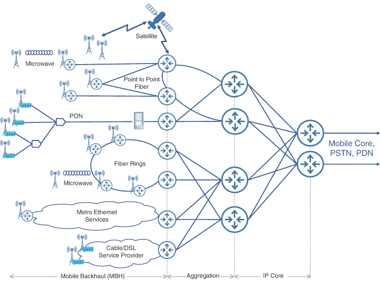
FIGURE 2-9 Cell Site Connectivity Models
Point-to-Point Fiber Connectivity
With the capability to carry massive amounts of data over longer distances, optical fiber has always been the preferred medium for transport networks. This also holds true for mobile backhaul networks where fiber connectivity could be extended from aggregation nodes to each cell site. The use of point-to-point fiber from each cell site to aggregation node is perhaps the best, albeit expensive, option to accomplish this task.
The dedicated fiber between the cell site and aggregation node(s) offers the highest bandwidth availability to and from the cell site, thus alleviating any scalability concerns resulting from increased data use from mobile subscribers. At the same time, it’s easier to upgrade to a higher capacity interface (for example, 10Gbps or 100Gbps), provided the transport devices at both the aggregation and cell sites support high-capacity interfaces. Additionally, any failures such as fiber cuts or cell site router failures are also localized between the two devices and do not impact other parts of the network.
The aggregation node, however, represents a single point of failure in the access domain for all cell sites connected to it. To alleviate this, as a best practice, aggregation nodes are deployed in pairs, and cell sites can be dual-homed to both aggregation nodes for redundancy. Both single-homed and dual-homed cell sites with point-to-point fiber links were previously shown in Figure 2-9.
The two aggregation nodes to which the cell sites are dual-homed are often, but not necessarily, co-located. The dual-homed connections from the cell sites to the aggregation nodes create a Clos architecture, creating an access fabric of dual-connected nodes. The same concept could be applied in the aggregation and IP core networks (see Figure 2-10).

FIGURE 2-10 Clos Fabric for Mobile Backhaul Networks
Clos Fabric
The term Clos fabric refers to a hierarchical, point-to-point connectivity design that creates a partial mesh topology between, and across, different network layers. Clos fabric offers a deterministic number of hops between various devices. It is extensively used in data center architectures and is covered in detail in Chapter 7, “Essential Technologies for 5G-Ready Networks: DC Architecture and Edge Computing.”
Point-to-point fiber to each individual cell site provides unparalleled architectural simplicity, flexibility, and scalability. However, the downside of such fabric-style, point-to-point fiber connectivity is its significant cost. The dedicated link for each site also requires a dedicated network interface on the aggregation node. This not only adds to the overall cost of the aggregation node(s), but also requires a larger, bulkier chassis (to accommodate a network port per cell site) that in turn needs more real estate for installation and consumes more power. This option also requires abundant fiber availability from aggregation nodes to every cell site, which could be challenging for large geographical areas. Oftentimes the projected cost of fiber deployment for an access fabric for MBH makes this option impractical.
To better balance cost and benefits, mobile operators have been exploring other options for MBH network design. One of these alternatives is to use fiber rings instead of point-to-point connections between cell site and aggregation nodes.
Fiber Rings
Fiber rings provide a healthy mix of cost and functionality in comparison to a point-to-point topology. In a ring-based deployment model, a number of cell sites are chained together, with each end of the chain connected to an aggregation node. The two aggregation nodes, marking the ends of this chain, may have a direct link between them, making it a closed ring as opposed to an open ring, where there is no link between the aggregation nodes. Both open and closed ring models are acceptable and widely deployed options, and both provide a redundant path to aggregation in case of a link failure on the ring. The ring topology depicted in Figure 2-9 is an open ring.
A ring-based topology operates with significantly fewer fiber links as compared to a point-to-point fiber connectivity model. Fiber rings also reduce the span of each fiber link, as the neighboring cell sites tend to be closer to each other than the aggregation node site. Therefore, rings allow the mobile service provider to connect a significantly higher number of cell sites with a lower fiber deployment cost. The cost savings, coupled with geographical coverage and built-in redundancy, make fiber ring topologies a favorite among mobile service providers for backhaul connectivity.
Fiber ring-based mobile backhaul deployments are not without their compromises. First and foremost, higher-capacity interfaces are required on the ring, as a plurality of cell sites share the same connection. Latency is another concern, as traffic from a cell site router now traverses more devices, and potentially longer distances, before getting to the aggregation node. The increased latency could have an impact on latency-sensitive services.
It’s hard to estimate how many cell sites are currently deployed using fiber rings, as providers tend not to publish this level of design and deployment choices, but it’s fair to say that ring-based topologies are overwhelmingly preferred by service providers for their MBH deployments.
Passive Optical Networks (PONs)
Developed as a last-mile access technology, passive optical networks (PONs) provide fiber access to the end user, who could be a residential subscriber, an enterprise, or, in the case of MBH, a cell site.
A PON operates as a two-device solution, consisting of an optical line termination (OLT, sometimes called an optical line terminal) and an optical network termination (ONT, also called an optical network unit, or ONU). The OLT resides at the aggregation site, whereas the ONT or ONU is the user-side device that, in the case of MBH, resides at the cell site.
ONT vs. ONU
The terms ONT and ONU are frequently used interchangeably, the difference being that ONT is used in ITU-T defined standards, while ONU is used by IEEE. An ONT was initially considered more feature-rich than an ONU, but that distinction is almost negligible today.13
This book will refer to the user-side equipment of a PON as ONT.
The optical network that connects the OLT and ONT, called the optical distribution network (ODN), uses a single strand of fiber with different wavelengths for upstream and downstream communication. An optical splitter, a passive mechanical device, splits this single strand of fiber from the OLT into 2, 4, 8, 16, or more branches to create point-to-multipoint connectivity between the OLT and ONT. The technology gets its name from the passive nature of the splitter; that is, it does not require any power to operate. Multiple optical splitters can be cascaded, resulting in flexible topologies to match a provider’s fiber availability. An OLT has multiple PON interfaces, with each one connecting to multiple cell sites, as shown in Figure 2-11.

FIGURE 2-11 Passive Optical Networks for Mobile Backhaul
There is a one-to-many relationship between the OLT and the ONT, where upon bootup, every ONT registers with its respective OLT and downloads its configuration. PON is a TDM-based technology, where an OLT acts as a “controller” for all the ONTs registered with it, providing each one with a timeslot for upstream and downstream communication.
PON has been an effective technology that brings fiber access to consumers and businesses at a reasonable cost to network operators. PON standards have evolved over the years to keep up with growing adoption and demands. Some of the popular PON variations are Gigabit PON (GPON), XGPON (10 Gig PON), Next Generation PON (NG-PON), and its subsequent evolution, NG-PON2. Each one of these standards extends the bandwidth available per PON port as well as the total number of subscribers that can be connected over a single port. GPON, for instance, offers 2.4Gbps downstream and 1.2Gbps upstream bandwidth with up to 64 nodes (128 in some cases) on a single GPON interface. NG-PON2, by contrast, offers 40Gbps downstream and 10Gbps upstream with a split ratio of up to 1:256 (that is, a single NG-PON2 port could support 256 ONTs).
The lower cost of the solution comes from the use of flexible fiber layout, as well as the cost of the equipment itself. The passive optical splitter is a low-cost, compact device that could be installed anywhere without having to worry about power availability. The ONT is an inexpensive optical-to-electrical converter with limited functionality that can often be implemented on a pluggable transceiver. A single PON interface on the OLT can terminate dozens of ONTs, further reducing the overall cost of a PON-based solution.
The total bandwidth of a PON interface is shared among all the ONTs connected to that interface. A higher split ratio means a larger number of ONTs connected on the same PON port, resulting in less bandwidth for each individual ONT. In an MBH network, this means the cell site’s throughput is dependent on the split ratio, with an inverse relationship between the split ratio used and total bandwidth available.
Microwave Links
All the mobile backhaul models discussed thus far require fiber connectivity all the way to the cell site. In many cases, however, getting fiber to a cell site might not be possible or feasible. Difficult terrain, unusually long distances to remote cell sites, high cost of deployment, challenges in obtaining necessary permits for fiber trenching, and meeting time to market goals are some of the reasons why a mobile network operator may forgo wired connectivity to cell sites in favor of wireless options.
One of the wireless options is microwave, a line-of-sight technology that uses directional antennas to transmit and receive traffic between two fixed locations. Using microwaves, the cell sites could either be connected directly to the aggregation nodes or daisy chained. Figure 2-12 shows sample mobile backhaul topologies using fiber and microwave.
FIGURE 2-12 Using Microwave Links for Mobile Backhaul
While fiber is the preferred connectivity option for MBH networks, microwave links offer an opportunity to extend connectivity to cell sites quickly and often at a lower cost. Microwaves do have considerable drawbacks in terms of link speed and stability. Because microwave requires direct line of sight, careful planning is essential to ensure there are no obstacles (natural or man-made) between microwave sites, taking into account future vegetation growth and construction plans. Microwave links are also susceptible to atmospheric conditions, and link performance could deteriorate in unfavorable weather conditions. Nonetheless, due to shortened deployment timelines and cost savings, microwave is a popular backhaul connectivity choice for mobile operators, even though microwave links provide significantly lower bandwidth compared to fiber links. A combination of fiber and microwave offers a mobile operator flexible options to create a backhaul topology. As of 2017, microwave links accounted for more than 56% of all MBH links due to widespread adoption of the technology in developing regions.14
Metro Ethernet Services
As Ethernet gained popularity, it created a growing need for standardized Ethernet services for metro and wide area networks. Metro Ethernet Forum (MEF), a nonprofit consortium of network operators and equipment vendors, was created in 2001 with an objective of expanding Ethernet from a LAN-based technology to a “carrier class” service over long distances.
MEF Certification
To help Ethernet become a reliable and robust form of WAN communication technology, MEF created standardized service definitions, established common terminologies, and devised service attributes. MEF also created a certification program, where equipment vendors and network operators can get their products and service offerings certified. The certification ensures that both the Metro Ethernet products as well service offerings adhere to the various service guidelines and attributes defined by MEF.
The services defined by MEF are commonly referred to as MEF services, Metro Ethernet services, or Carrier Ethernet Services and are broadly classified into three categories:
Ethernet Line (E-Line) services: Point-to-point services between two sites, similar to a leased line such as T1/E1.
Ethernet LAN (E-LAN): Multipoint services between multiple sites, similar to how multiple individual nodes communicate in a LAN.
Ethernet Tree (E-Tree): Rooted multipoint services where multiple end nodes communicate with a few select “root” nodes. The end nodes are not allowed to communicate between themselves directly, similar to legacy Frame Relay services.
MEF services operate independently of the underlying physical medium and topology and can be implemented over fiber rings, fabric, PON, or wireless technologies such as microwave. Figure 2-13 shows a view of these E-Line, E-LAN, and E-Tree services.

FIGURE 2-13 Metro Ethernet Services for Mobile Backhaul
Metro Ethernet services play a significant role in providing backhaul connectivity. Mobile operators that do not own their own transport can purchase Metro Ethernet services from data service providers, whereas the ones that do may implement MEF services to provide connectivity from cell sites to the rest of the network. A detailed implementation of MEF services is covered in Chapter 8, “Essential Technologies for 5G-Ready Networks: Transport Services,” and its application in mobile networks is discussed in Chapter 10, “Designing and Implementing 5G Network Architecture.”
Cable and DSL
Commercial Internet services such as cable and Digital Subscriber Line (DSL) are additional low-cost cell site connectivity options for backhaul networks. These technologies were originally designed to provide Internet access for residential and business subscribers and are geared toward best-effort quality of service with relatively low bandwidth.
Cable and DSL might be good connectivity options for smaller cell sites catering to a limited number of mobile subscribers but are not suitable for typical macrocell sites that offer mobile services over a larger geographical area. The use of cable and DSL in mobile backhaul has been steadily declining and being replaced with fiber or microwave.
Satellite
In rare cases, satellite-based communications from cell sites can be used for mobile backhaul. Traditionally, satellite backhaul has been a costly connectivity mechanism, offering lower speeds and higher latency, when compared to most of its terrestrial counterparts. Recent advancements in satellite technology have, to some extent, addressed the cost challenges. Latency, however, continues to be a major concern with satellite-based backhaul communications. Depending on the satellite orbit (low-earth, mid-earth, or geosynchronous), the round-trip latency from cell sites may range from tens to hundreds of milliseconds, which might not be feasible for latency-sensitive applications.
Satellite-based backhaul might be useful for some outlying cell sites due to their isolated or remote locations. Providers might also use satellites as a temporary, stopgap measure while building out their microwave or wired networks. Satellite links make up less than 2% of total backhaul links and are expected to remain a niche option for backhaul connectivity.15
Mobile Core Concepts
What started as a then-sophisticated mobile switching center in the first generation of mobile communication slowly transformed into a set of individual devices implementing multiple functions to provide the mobile services. These devices perform functions such as mobile device registration, processing and switching mobile traffic (both voice and data), implementing and managing subscriber policies, usage tracking, and billing support—essentially acting as the brain of the mobile network. This brain of the mobile communication network (MCN) is called “mobile core.”
The evolution of mobile core’s individual functional blocks has been extensively discussed in the previous chapter. This evolution of functionality was accompanied by changes to how mobile core devices are physically deployed and connected. For someone designing or implementing the RAN and MBH, the mobile core appears as a monolithic block that they are connecting to. However, in reality, the mobile core is geographically spread out.
In the initial days of cellular services, the mobile core (just the MSC and some databases at that time) served small geographical regions where they were deployed. Though these MSCs were initially connected using PSTN, data technologies such as Frame Relay, ATM, and eventually IP/Ethernet started to dominate this connectivity landscape over subsequent years. Mergers of many data network providers and mobile service providers further bolstered this transition through reduced cost of long-haul data links that could meet the growing bandwidth demands of inter-MSC communication. Mobile providers therefore started using leased (or owned) data links to connect the geographically spread mobile core devices.
The distributed nature of this mobile core resulted in higher deployment, management, and maintenance costs. To lower that expense, mobile operators found it attractive to try consolidating the data centers hosting mobile core devices and reducing the devices’ footprint. There were a few key challenges that initially hindered such consolidation:
The subscriber scale supported by the mobile core devices would limit the coverage area per device.
The cost associated with backhauling the traffic from the cell site to mobile core would increase with distance.
Due to their higher serialization delays, the lower capacity links would result in higher latency and degraded user experience.
Over the years, multiple factors and innovations contributed to overcoming these challenges. The multifold increase in devices’ capacity and performance allowed a fewer number of mobile core devices to serve subscribers over a larger geographical region. At the same time, technological improvements resulted in higher-bandwidth links with lower serialization delays, which made it possible to cover larger distances within the same latency budget. Business mergers yet again supported the transition as the cost of backhaul connectivity decreased with network consolidations. The resulting reduction in mobile core footprint and its geographical consolidation still required an optimal balance between backhaul cost, device scalability, and network latency to be considered. Therefore, the RAN-facing devices had limited room for consolidation due to these limiting factors. On the other hand, devices, such as databases and authentication servers, implementing functions internal to the mobile core could be consolidated even further into a few central locations.
The resulting architecture is a geographically distributed mobile core, with some devices in centralized data centers, with other devices in data centers forming the periphery of this distributed mobile core. PSTN, PLMN, and PDN gateways were also consolidated to select locations on this periphery—determined based on requirements and traffic load of the various geographical markets. Figure 2-14 shows this geographical deployment layout of the mobile core.
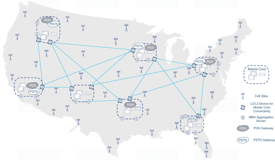
FIGURE 2-14 A Geographical Layout of a Mobile Core
By the third generation of mobile networks, the functions within the mobile core could be broadly placed into three categories:
Voice traffic signaling, processing, and switching
Data traffic signaling, processing, and forwarding
Databases to store subscriber information and usage details
As voice traffic was historically handled using circuit switched networks, the part of the mobile core performing those functions was dubbed circuit switched core. On the other hand, starting with 2.5G, the data traffic functions were implemented as a packet switched network and consequently dubbed packet switched core, or simply packet core. The databases supporting the functions such as user registration and authentication continued to be part of the circuit switched core, even though the packet core also made use of them.
Circuit Switched Core
Up until 3G, the voice traffic in mobile networks was circuit switched, with the MSC performing the functions of user registration, call routing and establishment, switching the voice circuit between end users, intra- and inter-provider roaming, and so on. For calls that originated or terminated outside the provider network, Gateway-MSC (G-MSC) were used—which would perform all the regular MSC functions and additionally connect with the PSTN. In later releases of 3G, the MSC was split into MSC-Server (MCS-S) and Media-Gateway (MGW). The MSC-S inherited the signaling responsibilities of the MSC, while the voice circuit was established via MGWs. In 3G, IP started to take center stage to interconnect MSCs, or rather their 3G equivalents—MGW and MSC-S. This resulted in new frameworks such as SIGTRAN that defined the use of SS7 protocols over IP transport. However, the use of circuit switched voice continued to exist and hence the name “circuit switched core.”
Visited MSC (V-MSC) and Gateway MSC (G-MSC)
All MSCs in the 2G network have the responsibility to manage multiple base station controllers. These MSCs are interconnected and can route calls to and from the mobile handsets that are registered to it. For calls that originate or terminate from networks outside the mobile provider’s network (for example, PSTN and other mobile providers), a small subset of these MSCs has connectivity to external networks and acts as a gateway to those networks. Consequently, these MSCs are referred to as Gateway MSC (G-MSC). The MSC where a mobile subscriber is registered is referred to as Visited MSC (V-MSC) for that subscriber. The G-MSCs still serve as V-MSCs for the BSCs they manage but perform the additional functions of gateways to external networks.
Identifiers and Databases in Mobile Networks
The user registration and communication flow makes use of various identifiers. The identifiers used are stored in various databases as well as the SIM card and mobile handset.
Subscriber Identification Module (SIM) Card
GSM introduced the concept of the SIM card, which is a small card with a microcontroller and memory built into it. SIM cards are meant to securely store the user’s identifying information and provide that information to the mobile service provider when authenticating and registering the user. A subscriber can therefore use the mobile service by plugging their SIM card into any compatible mobile device.
Figure 2-15 shows where these identifiers were originally stored.

FIGURE 2-15 Owners of Key Identifiers in a Mobile Network
Table 2-2 summarizes the identifiers and their use.
TABLE 2-2 Summary of Identifiers Used in Mobile Communication Network
Identifier | Description and Purpose |
|---|---|
Integrated Circuit Card Identifier (ICCID) | The ICCID is used to uniquely identify a SIM card. It’s up to 22 digits long—starting with “89,” representing the Telecom Industry. The ISSID is followed by Mobile Country Code (MCC), Mobile Network Code (MNC), a provider-generated serial number, and a single-digit checksum (C). |
International Mobile Subscriber Identity (IMSI) | IMSI uniquely identifies a mobile subscriber and is assigned upon signing up for the mobile service. IMSI is typically 16 digits long, comprising the MCC, MNC, a unique serial number generated by the provider called the mobile subscriber identification number (MSIN), and finally a single-digit checksum. IMSI is securely stored within the SIM card’s memory as well as the mobile provider’s databases. |
International Mobile Equipment Identity (IMEI) | IMEI is a unique 15-digit number associated with a mobile device. The first eight digits of IMEI, referred to as the type allocation code, encodes information about the device manufacturer and model number. These are followed by a serial number specific to the manufacturer (six digits) and finally a check digit to verify the integrity of the other values. IMEI can be used to track and/or block stolen and grey market devices from connecting to the mobile network. |
Home Network Identity (HNI) or Public Land Mobile Network (PLMN) | The service provider is uniquely identified using the combination of MCC and MNC values. This value is referred to as HNI or PLMN. |
Mobile Station International Subscriber Directory Number (MSISDN) | The MSISDN is what the mobile subscribers generally refer to as their phone number. It is mapped to the IMSI in the mobile provider’s database. The MSISDN comprises a country code (up to three digits), a national destination code (up to three digits), and a subscriber number that can be up to 10 digits long. |
Mobile Station Roaming Number (MSRN) | To facilitate the routing of calls within the mobile core, the visiting MSC assigns a temporary number to the subscriber, called the MSRN. It is locally significant within the network of the provider and uses the same format as the MSISDN. |
Temporary Mobile Subscriber Identity (TMSI) | TMSI is a temporary identity assigned to the mobile subscriber to use in lieu of the IMSI, which is kept secret and used only during registration to secure the privacy of the subscriber from eavesdroppers. |
Local Mobile Station Identity (LMSI) | LMSI is another temporary value assigned to the subscriber with the purpose of acting as a pointer to the database for faster IMSI lookup. |
Cell Identification (CI) value | CI is a byte value that uniquely identifies a cell site. |
Location Area Code (LAC) and Location Area Identifier (LAI) | The cells in the mobile network are grouped together into location areas, and a 16-bit identifier called the LAC is used to represent that area. The LAC, MCC, and MNC are broadcasted as a single value referred to as the LAI. |
Figure 2-16 illustrates the format of these identifiers.

FIGURE 2-16 Formats for Key Identifiers in a Mobile Network
In the mobile core, the four mentionable databases where these identifiers are stored are the HLR, VLR, AuC, and EIR, as described in the sections that follow.
Home Location Register (HLR)
The Home Location Register (HLR) was introduced in the previous chapter as a database containing information of all the mobile users. Expanding that definition further, the HLR is the mobile service provider’s master database where a subscriber’s information is populated upon signing up for the service. This information includes the subscriber’s phone number (MSISDN), the IMSI value allocated, types of services subscribed, permissions and privileges, and authentication information. Additionally, the HLR also stores some runtime information about the subscriber, such as knowledge of the MSC currently serving the subscriber.
There are usually just a handful of HLR nodes across the mobile provider’s network, and these are geographically distributed. All MSCs communicate with HLR in their network to pull subscriber information.
Visited Location Register (VLR)
In contrast to HLR, the Visited Location Register (VLR) databases are individually associated with each MSC. In fact, VLRs have been typically bundled within the MSC hardware instead of being implemented as separate database servers. When a user enters any MSC’s coverage area, making it the Visited MSC (V-MSC), that V-MSC queries its local VLR for information to authenticate, register, and authorize the user. The VLR entries are temporary and will contain information only about the subscribers that are either currently or were recently registered with its associated MSC. If the user information does not already exist in the VLR, it reaches out to the HLR and copies over the subscriber information to its own database. This makes the VLR a sort of cache database for HLR, hence reducing the number of queries that V-MSCs would need to send toward the HLR. Regardless of whether the user information is already present in the local VLR or needs to be fetched from the HLR, the V-MSC always informs the HLR when it registers the user. This helps the HLR to keep track of which MSC is serving as the subscriber’s V-MSC. When any other MSC, including the G-MSC, receives a call meant for that user, it can consult the HLR for the V-MSC information to route the call to that V-MSC.
VLR also allocates some local temporary parameters to the user, some of which are copied to HLR. Figure 2-17 shows a high-level view of the information stored in the HLR database and VLR databases as well as the permanent fields that are copied from HLR to VLR upon user registration.

FIGURE 2-17 HLR and VLR Entries at a Glance
Among the identifiers mentioned previously, the TMSI, LMSI, and LAI/LAC are allocated by the V-MSC locally and stored in its own VLR, as depicted in Figure 2-17. MSRN is also locally assigned, but because the rest of the network needs to be made aware of this number being assigned to the subscriber (for calls to be routed to the V-MSC), the MSRN value is copied over to the HLR as a temporary piece of information mapped to the IMSI of that subscriber.
Authentication Center (AuC)
The Authentication Center was previously mentioned as the database that facilitates authentication and authorization of mobile subscribers. Specifically, it stores unique key values mapped to each subscriber’s IMSI. A copy of that key is also safely stored in the user’s SIM card. When validating the subscriber’s identity, the VLR queries the HLR, which then communicates with the AuC. The AuC uses the key stored against the user’s IMSI to authenticate the user. This key is also used by the mobile device and the AuC to generate a cipher for encrypting radio communication.16
Equipment Identity Register (EIR)
This purpose of the Equipment Identity Register (EIR) is to verify the equipment being used by the subscriber. The EIR stores the devices’ IMEI that may be explicitly allowed or restricted on an operator network. Some of the information in EIR may include the IMEI values for mobile devices that have been reported as lost, stolen, fraudulent, or illegal. During the authentication process, the IMEI of the user’s device is cross-checked against the EIR stored values to ensure that the device should be allowed to register with the mobile network.
User Registration and Call Flow
The subscriber information initially exists only in three places—the HLR and AuC of the service provider as well as the SIM card provided to the subscriber. Once the subscriber plugs the SIM card into a mobile device and turns it on, the device scans its supported frequencies for carrier information broadcasts, which includes, among other parameters, the PLMN (MCC+MNC) of the service provider. The mobile device will also read the SIM card’s ICCID and match the PLMN values from the SIM card to the PLMN values in the broadcasts. If a match is found, the device continues to the registration process. If a match is not found (that is, the subscriber is not within the coverage area of its service provider), the selection process randomly chooses other available PLMN values and attempts the registration process. For a selected PLMN, the mobile handset sends the IMSI (extracted from the SIM card) and the IMEI of the device as part of the registration request.
The MSC that receives this information (V-MSC) checks if its VLR records contain information about this IMSI. If it doesn’t, the HLR is consulted to verify that the IMSI value is authorized to use cellular services. The HLR ensures that the IMSI belongs to an existing subscriber and then passes the IMSI to its corresponding AuC to authenticate the user. At the same time, it checks the EIR to ensure that the IMEI of the user’s device is not in any list that is not allowed to register.
AuC looks up the subscriber’s secret key using the IMSI value and then performs a 128-bit hash on a randomly generated number using that key. It passes the result of that encryption back to the HLR along with the random number used. This random number is sent to the subscriber as a challenge, where the hash is now performed by the SIM card using the key stored on it. Results of both hash calculations—the one performed by AuC and that performed on SIM card—should be identical as long as the key values match. Hence, the hash calculations from the SIM are sent to the V-MSC, which compares these values and completes the authentication process if there is a match.
Once the subscriber is authenticated, the subscriber’s static information from the HLR is copied over to the local VLR. Additionally, the HLR is updated about the MSC where the subscriber is registered (that is, the V-MSC). The V-MSC will also allocate the TMSI identifier (to be used for subsequent communication with the mobile handset) and notify the device about its current TMSI value. The MSRN is also allocated and populated in the VLR and HLR databases.17
To complete the registration, the mobile handset updates the V-MSC about its selected LAI and CI values. This helps the V-MSC keep track of the cell tower being used. At this point, the device is ready to make and receive phone calls. Interestingly, the device doesn’t need to know its own phone number (MSISDN). Instead, the IMSI/TMSI values identify the subscriber to the MSC, which then maps these to the subscriber’s MSISDN for outgoing calls. Figure 2-18 summarizes this subscriber registration process.
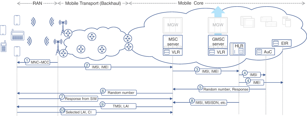
FIGURE 2-18 Subscriber Registration Process
Once the subscriber is registered with the network, the HLR keeps track of the V-MSC/VLR serving this subscriber. For any incoming call for this subscriber’s MSISDN number, whether originating within or outside the mobile provider’s network, the G-MSC will be consulted to route the call. For calls within the network, the G-MSC notifies the caller’s MSC about the called subscriber’s MSRN. The MSRN can then be used to route the call to the V-MSC. If the call has originated in a different telephony network, the G-MSC will use the MSRN to route the call to the V-MSC. At the same time, a bearer channel is established between the V-MSC and the caller’s MSC (or G-MSC, if the call originated from outside the PLMN). In both cases, the V-MSC will send a call-setup message to the subscriber’s TMSI, within the currently known area of the subscriber (using the LAI value stored in the VLR). Once the call is confirmed by the callee’s device, a bearer channel is established over the air interface between the callee’s device and the V-MSC. Figure 2-19 shows this call-setup process.

FIGURE 2-19 End-to-End Call Flow
For calls made by the subscriber, initially the mobile device requests allocation of a bearer from the mobile network. Once the bearer is provided, the caller’s V-MSC determines reachability to the dialed number by consulting the G-MSC. If this number is outside the network, the call is routed to the G-MSC, which can then route externally. If the number is registered with the network, the previously described steps take place.
Packet Switched Core
Although the first two generations of mobile networks were voice-centric and did not offer dedicated data transmission service, it was still possible to use data by establishing a modem connection to a remote fax machine or email server. The data rates for such modem connections were much lower compared to dial-up over PSTN.
Data speeds were slightly improved by making 2G networks aware of data transmission within a circuit switched connection. Indeed, a 2G mobile device didn’t feature a real modem. The mobile devices used a traffic adaptation function instead to fit the data transmission into a digital traffic channel while the actual modulation and demodulation happened at the MSC. Although this helped to achieve data transmission speeds of 14.4Kbps over a single traffic channel or even 57.6Kbps over multiple concatenated timeslots, a significant innovation was needed to boost data transmission rates and capabilities of the mobile network. It was inevitable that circuit switched data would be replaced by packet switched data communication in the mobile core.
Packet Switched Data
The technological jump from circuit switched data communication to packet switched required significant mobile core innovations and new functions. These new functions were separated from MSC in second-generation (2G) mobile networks and implemented as new nodes for scalability and efficiency. These nodes were collectively called the General Packet Radio Service (GPRS) sub-system (GSS) and became the foundation of what was later dubbed a “packet core” in 3G networks. In addition to GSS, a typical packet core uses other supplementary components such as Domain Name System (DNS) servers, Dynamic Host Configuration Protocol (DHCP) servers, and Authentication Authorization Accounting (AAA) servers.
The GPRS sub-system did not significantly change in 3G, save for some enhancements to allow 3G-specific interfaces and flows. Even in the fourth-generation (4G) mobile networks (which will be discussed in the next chapter), many GSS components can be easily identified, albeit with some changes in node names and certain functions redistributed.
GPRS Sub-System (GSS)
GSS comprises two GPRS support nodes (GSNs) called the Serving GPRS Support Node (SGSN) and Gateway GPRS Support Node (GGSN). Collectively, the GSN implement functions critical for packet switched data services such as preparation of data packets for transmission over the air interface, routing, traffic management, data encryption/decryption, and IP address allocations. This is in addition to other mobile functions (for example, subscriber tracking across different cells or roaming to other networks, billing, and lawful intercept).
SGSN’s primarily role is to control the subscriber’s session and data packet delivery between the mobile phone and mobile core. GGSN, on the other hand, is responsible for grooming and routing data packets to and from the Internet, intranets, or other external packet networks and mobile core. In other words, whereas SGSN is the mobile-phone-facing node, GGSN is a gateway between external packet networks and the mobile core. Simply put, SGSN provides session management, whereas GGSN provides connectivity to the Internet and other data networks.
While physically SGSN looks more like yet another rack with modules and various interfaces, it is common for a GGSN to be implemented using an IP router with specialized modules and interfaces to communicate with the rest of mobile core.
SGSN, GGSN, and PDP Context
Before a mobile subscriber can use data service, a series of exchanges has to take place between the mobile phone, GPRS sub-system, and other components of the mobile core. A mobile device’s request for data service triggers an SGSN inquiry into the HLR to authenticate and authorize use of network resources by the subscriber. SGSN also notifies the HLR about the subscriber’s location.
Once the subscriber is attached to the network, the mobile device has to negotiate additional parameters to access data services. These include the type of PDN it is allowed to access (public vs. private), QoS policies, and IP address allocation. Collectively, these parameters along with the assigned billing profile comprise a subscriber-specific Packet Data Protocol (PDP) context.
Note
The PDP context may be perceived as a subscriber’s data profile, defining what PDNs can be accessed and how. The PDP context is an essential construct to bring data connectivity to the mobile device.
The request for PDP context activation is sent by a mobile device to its serving SGSN, and the SGSN must forward this request to a GGSN. A typical mobile network has a number of GGSNs deployed, with each GGSN providing access to one or more PDNs. Depending on the request, the SGSN selects the appropriate GGSN to forward this request.
Among other parameters, a PDP context activation includes an access point name (APN), which is akin to a fully qualified domain name (FQDN) in data networks. An APN serves as a reference to a particular GGSN and a specific PDN connection within that GGSN. The APN scope is limited to the collection of PLMN networks bound by roaming agreements and has no meaning outside of it.
Access Point Name (APN)
A typical APN might look like the following string: internet.operatorname.gprs. It can be viewed and changed in the mobile device settings and, in most cases, is automatically pulled from a subscriber’s SIM card. It is not uncommon for a phone to have more than one APN configured and used.
SGSN resolves the requested APN to a GGSN’s IP address using PLMN internal DNS servers and sends the request to activate PDP context to this GGSN. In turn, GGSN may consult with AAA server to ensure a user is authorized to use a particular PDN and, upon successful authorization, allocates an IP address to the mobile device using a local or external DHCP server. Once the PDP context is created, the GGSN responds back to the SGSN with the PDP context, including the IP address, and is ready to route packets between mobile device and the respective PDN. GGSN also maps the session to QoS profiles and ACLs. Figure 2-20 shows the PDP context activation process and GPRS data flows.

FIGURE 2-20 GPRS Data Flows
The PDP context in the SGSN–GGSN pair remains active as long as the GPRS subscriber is attached and reachable. When a mobile device roams into another SGSN serving area, the “new” SGSN pulls the existing PDP context from the “old” SGSN and updates the HLR with the new location. The parameters associated with the PDP context (such as the IP address) stay the same, even though the subscriber is now being served by a new SGSN.
With PDP context activated, the network is now ready to provide data services. When the subscriber starts exchanging data with the PDN, both the SGSN and GGSN generate charging tickets and supply usage data to the billing system. Additionally, the SGSN and GGSN can be a point of lawful intercept functions.
If a mobile device moves out of reach and remains unreachable for a certain time duration, it is detached from the GPRS network and the PDP context is deactivated. A mobile device can also voluntarily request a GPRS detach, and once this is completed, it can no longer send or receive data until it reattaches to the GRPS network.
GPRS Interfaces
These sophisticated series of communications between multiple mobile core entities require a number of interfaces and protocols. Earlier mobile core entities were not IP-enabled and used many legacy protocols and interfaces from the circuit switched world. Being new and based on packet switching, the GPRS sub-system adopted IP for communications between SGSN, GGSN, and supplemental DNS AAA and DHCP servers. Yet, they needed to support other interfaces and protocols to communicate with other mobile core nodes.
Note
In the mobility world, the term interface is also used to define connectivity reference points, as defined by 3GPP. These are meant to standardize communication between various functions.
Figure 2-21 provides a view of GPRS interfaces with their relation to mobile core nodes. The shaded area represents the packet core.

FIGURE 2-21 Protocols and Interfaces of a GPRS Subsystem
The few mentionable interfaces are Gi and Gn/Gp. Gi is an IP interface and connects the GGSN to the external PDN, such as the Internet or intranets. Gn and Gp interfaces connect the SGSN and GGSN and are very similar in nature. While the Gn interface connects the SGSN and GGSN belonging to the same PLMN, the Gp interface provides connectivity between the SGSN and GGSN in different PLMNs. These interfaces used IP over ATM as the transport in some early implementations but have since moved to IP over Ethernet.
The figure also highlights some of the protocols used in GPRS. Base Station Subsystem GPRS Protocol (BSSGP) is used to transport data units of upper protocols and layers between SGSN and PCU components of the BSC. These data units are then relayed by the PCU/BSC to mobile phones using Radio Link Control/Medium Access Control (RLC/MAC) over the air interface. Upper layer protocols used over BSSGP are SubNetwork Dependent Convergence Protocol (SNDCP) and Logical Link Control Layer (LLC). This tandem is used to reliably transport data units belonging to different subscribers, all the way to their mobile phones, as these layers extend from the SGSN beyond the BSC and reach the mobile phones.
GPRS Tunneling Protocol (GTP)
Despite both the subscriber’s data and GGSN-SGSN communication happening over IP, it is not feasible to use a subscriber’s IP address for routing inside the packet core for several reasons. Instead of using IP natively, the subscriber’s IP packets are transported in a tunnel between the SGSN and GGSN, using GPRS Tunneling Protocol (GTP) to provide traffic isolation. GTP tunnels also help avoid routing complications within the packet core and shield the subscriber’s data sessions from changes when a user moves between different SGSNs. When a serving SGSN changes, it pulls the existing PDP context details from the “old” serving SGSN and updates the corresponding GGSN. This way, no changes are required in the packet core IP transport routing protocols, and the subscriber’s IP address can stay unchanged during handovers. Figure 2-22 shows GTP tunnels established between GSNs.

FIGURE 2-22 GTP Tunnel Between GSNs
GTP is a TLV-based protocol, and besides transporting user data it is also used to deliver many types of control messages to establish and tear down tunnels, exchange information between GSNs, and so on. GTP also supports keepalive messages between GSN nodes to verify if their counterparts are alive and responsive.
A new GTP tunnel between the SGSN and GGSN is created each time a PDP context is activated. A subscriber might have multiple GTP tunnels and certain fields within the GTP frame (such as Flow Label and Tunnel Identifier, or TID), which can be used to uniquely identify the tunnel, subscriber, and the PDP context for transported data.
The initial release of the GPRS specification defined version 0 of GTP, which supported transport over both TCP and UDP with a well-known port of 3386. Because the same port number is used for all GTP communications in version 0, the only way to distinguish whether the GTP packets are carrying encapsulated subscriber datagrams, or signaling messages, is to look at the TLV values and the reference interface a packet belongs to (the Gn, Gp, or Ga interface).
In Release 99, GTPv1 was defined as a new version of GTP, bringing additional TLVs for signaling and replacing TID with Tunnel Endpoint ID (TEID). GTPv1 also distinguishes GTP-C for control plane traffic and GTP-U for data. UDP and TCP port numbers were also changed to 2123 for GTP-C and 2125 for GTP-U.18 Even though GPRS was defined in 2G with GTPv0, today GTPv1 is used in 2G, 3G, and partially in 4G networks. 3GPP introduced GTPv2 in Release 8, which included enhancements in the control plane (that is, GTPv2-C), while leaving the user plane intact.19
Although earlier releases specified support for GTP over both TCP and UDP, the majority of implementations favored UDP. This resulted in the removal of TCP support for GTP-C and GTP-U protocols from 3GPP specifications.20
With the evolution of mobile networks through the third and fourth generations, the amount of data traffic consumed by mobile subscribers grew exponentially, resulting in much higher bandwidth requirements within the mobile core. The GTP traffic awareness becomes critical for mobile core transport, as it often relies on load-balancing mechanisms over link bundles to provide the required bandwidth. A network gear’s ability to peek inside GTP packet headers and extract flow information allows for an even distribution of traffic over multiple links.
GSN Enhancements in 3G Core
Packet core composition did not significantly change in third-generation mobile networks. SGSN and GGSN preserved their key role in handling subscribers’ data traffic, keeping a number of G reference interfaces (Gn/Gp, Ga, and so on) untouched. Those G interfaces, used to interconnect packet core and circuit switched core entities, expanded their physical transport options with Ethernet and adopted use of the SIGTRAN (SS7 over IP) signaling framework. Otherwise, changes in the packet core were limited mainly to the new interfaces between UTRAN (the RAN component for 3G) and packet core. 3GPP initially proposed the use of ATM as a transport for new interfaces in UMTS specifications, with IP transport being added in later releases. Figure 2-23 shows interfaces interconnecting various components of the packet core (shaded area) and other mobile network entities as well as new interfaces introduced in UMTS.
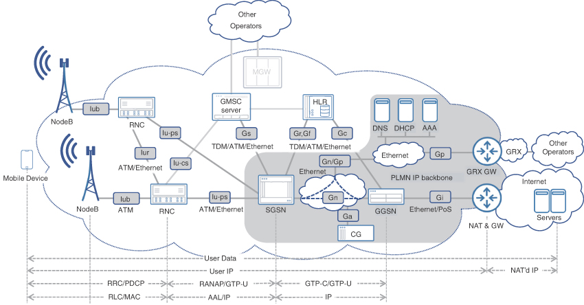
FIGURE 2-23 Protocols and Interfaces of 3G Packet Core and UTRAN
Two notable interfaces defined to connect UTRAN to the mobile core were Iu-CS (for RNC-to-MSC/MGW connections) and Iu-PS (for RNC-to-SGSN connections). These two interfaces carry both control and user traffic. The control plane uses a protocol named Radio Access Network Application Protocol (RANAP), which runs on SS7 over ATM. Use of SIGTRAN also became an option later. The user plane of Iu-CS either uses ATM or RTP over IP transport.
Particularly significant is the use of the GTP-U protocol for user traffic by the Iu-PS interface. Although it might seem like the GTP-U tunnel extends all the way from GGSN to RNC, in reality SGSN acts as a relay between GGSN–SGSN and SGSN–RNC GTP-U tunnels. Later 3GPP releases provided an option to establish a direct GTP tunnel between GGSN and RNC. It must be noted that a direct GTP tunnel can only be established within an operator’s network and cannot be used in inter-operator roaming scenarios. More details on GPRS roaming are covered in the next section. Figure 2-24 shows GTP-U tunnels with and without the direct tunneling option.
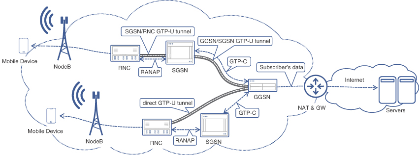
FIGURE 2-24 GTP-U Tunnels With and Without Direct Tunneling Option
For the sake of completeness, it is worth mentioning the Iur and Iub interfaces of UTRAN. The Iur interface is used to support handover and signal macrodiversity features (briefly described in Chapter 1, “A Peek at the Past”). Iub is the interface that connects RNC and NodeB and transports necessary signaling and subscribers’ voice and data. Both interfaces are primarily implemented over Ethernet today.
GPRS Roaming eXchange (GRX)
If allowed by the operators’ agreement and the subscriber’s profile, a mobile user can get data services on a visited network, and GTP plays an essential role in it. The process of registration on the visited GPRS network is very similar to what was described in the previous sections; however, a few important distinctions exist. When a roaming mobile device requests a PDP context activation, the SGSN on a visited network establishes a GTP tunnel to the home network’s GGSN. It is the home network’s GGSN responsibility to provide the subscriber with an IP address and access to the requested PDN. In other words, if a subscriber from North America accesses the Internet while roaming on a European mobile network, this subscriber’s IP packets appear to an Internet server as if they were coming from North America.
An operator’s SGSN can establish a GTP tunnel to another operator’s GGSN as long as the packet cores of both operators are interconnected. GPRS Roaming eXchange (GRX) is the most common way to establish such a connection. The concept of a GRX is similar to what Internet service providers use to interconnect their networks via transit networks and Internet peering exchanges. The GRX is usually operated by a private company and provides IP prefix information exchange, transit of IP traffic between different mobile operators, and root DNS service for GPRS.
IP Addressing and GRX
For security reasons, GRX networks are isolated from the Internet, which naturally reduces the risk of various attacks on GPRS nodes. Despite this isolation, GSN interfaces in the packet core typically use globally routable IP addresses to prevent IP address overlap between multiple operators. The GRX gateway connects the GSN’s Gp interfaces as well as DNS to the GRX networks and advertises some of the packet core’s IP subnets to the GRX network using Border Gateway Protocol (BGP). IP subnets and BGP autonomous system numbers are allocated to the mobile service providers by regional Internet registries in exactly the same manner and from the same IP addressing space used by the Internet.
DNS operation is essential for GPRS roaming, as it resolves the APN supplied by a roaming mobile device during PDP context activation request. The DNS on the visited network queries a root DNS server, which normally resides on the GRX operator’s network. The root DNS server then returns a referral to an authoritative DNS. Finally, the authoritative DNS resolves the APN to an IP address of the GGSN server in the home network.
Figure 2-25 illustrates a typical data roaming scenario. Notice that the DNS on the GRX is completely isolated from the DNS on the Internet for security purposes.

FIGURE 2-25 Data Roaming Flows via GRX
Evolving mobile services have diversified inter-operator traffic, which now includes packet voice and signaling, data traffic between mobile subscribers and content providers, and bulky GPRS roaming traffic. Inter-operator exchange of new traffic types requires improved security, services isolation, and differentiated SLAs. Naturally, a new type of inter-operator traffic exchange service emerged to meet new demands: IP eXchange (IPX). IPX is similar to GRX in many respects, but unlike its predecessor, it supports multiple SLAs for different traffic types, end-to-end QoS, improved security, and traffic separation. In fact, GRX traffic is defined as just one of the traffic types for an IPX. Nevertheless, it is not uncommon to see exchange providers advertising transit services as GRX/IPX. Most of inter-operator traffic today is transported over GRX/IPX exchanges.
Summary
This chapter expanded on the composition of the three mobile communication network domains: radio access networks, mobile backhaul, and mobile core.
For the radio access network (RAN), the following key factors were covered:
RF spectrum, various band properties, and optimal band selection
RF duplexing mechanisms
Cell splitting and sectoring
Key components of a cell site and cell site types
Mobile backhaul focused on the following key factors:
The role of mobile backhaul networks from the perspective of data network and mobility network architects
Historical insights and transition to Ethernet/IP-based backhaul
Various connectivity models for mobile backhaul networks
Mobile core’s concepts and details were discussed with an emphasis on the following:
Main elements of a mobile core and distinction between circuit switched core and packet core
Identifiers and databases used in mobile core
Packet core entities, interfaces, and important communication flows
The next chapter will discuss how the mobile communication networks have evolved across all three domains to create a more cohesive, efficient, and scalable end-to-end network.
References
1. https://auctiondata.fcc.gov/public/projects/auction107 (last visited: Feb 2022)
2. https://www.ntia.doc.gov/files/ntia/publications/2003-allochrt.pdf (last visited: Feb 2022)
3. https://transition.fcc.gov/oet/spectrum/table/fcctable.pdf (last visited: Feb 2022)
4. https://auctiondata.fcc.gov/public/projects/auction107 (last visited: Feb 2022)
5. https://www.etsi.org/deliver/etsi_ts/136100_136199/136101/16.07.00_60/ts_136101v160700p.pdf, Table 5.5-1 (last visited: Feb 2022)
6. Ibid.
7. https://www.etsi.org/deliver/etsi_ts/138100_138199/138104/16.05.00_60/ts_138104v160500p.pdf, Table 5.2-1 (last visited: Feb 2022)
8. http://www.cpri.info/downloads/CPRI_v_7_0_2015-10-09.pdf (last visited: Feb 2022)
9. https://www.businessinsider.com/reliance-jio-tower-asset-sale-indicative-of-industry-trend-2019-12 (last visited: Feb 2022)
10. https://portal.3gpp.org/desktopmodules/Specifications/SpecificationDetails.aspx?specificationId=910 (last visited: Feb 2022)
11. https://www.statista.com/statistics/185854/monthly-number-of-cell-sites-in-the-united-states-since-june-1986/ (last visited: Feb 2022)
12. https://www.businessinsider.com/reliance-jio-tower-asset-sale-indicative-of-industry-trend-2019-12 (last visited: Feb 2022)
13. James Farmer, Brian Lane, Kevin Bourg, and Weyl Wang. FTTx Networks: Technology Implementation and Operation (Cambridge, MA: Morgan Kaufman, 2017), Chapter 1
14. “GSMA Mobile Backhaul Options: Spectrum analysis and recommendations,” https://www.gsma.com/spectrum/wp-content/uploads/2019/04/Mobile-Backhaul-Options.pdf (last visited: Feb 2022)
15. Ibid.
16. https://portal.3gpp.org/desktopmodules/Specifications/SpecificationDetails.aspx?specificationId=1692 (last visited: Feb 2022)
17. Martin Sauter. From GSM to LTE-Advanced Pro and 5G: An Introduction to Mobile Networks and Mobile Broadband, Third Edition (Hoboken, NJ: Wiley, 2021), Section 1.8.2
18. https://www.3gpp.org/ftp/Specs/archive/29_series/29.060/29060-330.zip (Last visited: Feb 2022)
19. https://portal.3gpp.org/desktopmodules/Specifications/SpecificationDetails.aspx?specificationId=1692 (last visited: Feb 2022)
20. https://www.3gpp.org/ftp/Specs/archive/29_series/29.060/29060-3a0.zip (last visited: Feb 2022)