
Confidence bounds in social sensing
Abstract
In the previous chapter, we reviewed a maximum likelihood estimator (MLE) to jointly estimate the reliability of sources and determine the correctness of facts concluded from the data. However, an important problem that remains unanswered from the MLE approach is: what is the confidence of the resulting source reliability estimation? Only by answering this question, can we completely characterize estimation performance, and hence source reliability in social sensing applications. This chapter reviews analytically-founded bounds that quantify the accuracy of such MLE in social sensing. It is shown that the estimation confidence can be quantified accurately based on both real and asymptotic Cramer-Rao lower bound (CRLB). Additionally, this chapter also reviews an estimator on the accuracy of claim classification without knowing the ground truth values of the claims.
6.1 The Reliability Assurance Problem
In this chapter, we introduce a reliability assurance problem in social sensing, where the estimation-theoretic approaches are used to quantify the accuracy of the maximum likelihood estimation (MLE) framework presented in the previous chapter [103, 104]. In particular, the goal is to demonstrate, in an analytically-founded manner, how to compute the confidence interval of each source’s reliability. Formally, this is given by:
(ˆtMLEi−clowerp,ˆtMLEi+cupperp)c%i=1,2,…,M
where ˆtMLEi![]() is the MLE on the reliability of source Si ,c% is the confidence level of the estimation interval, clowerp
is the MLE on the reliability of source Si ,c% is the confidence level of the estimation interval, clowerp![]() and cupperp
and cupperp![]() represent the lower and upper bound on the estimation deviation from the MLE ˆtMLEi
represent the lower and upper bound on the estimation deviation from the MLE ˆtMLEi![]() , respectively. The goal is to find clowerp
, respectively. The goal is to find clowerp![]() and cupperp
and cupperp![]() for a given c% and an observation matrix SC. It turns out that the Cramer-Rao lower bounds (CRLBs) of the MLE on the source reliability need to be computed in order to obtain the clowerp
for a given c% and an observation matrix SC. It turns out that the Cramer-Rao lower bounds (CRLBs) of the MLE on the source reliability need to be computed in order to obtain the clowerp![]() and cupperp
and cupperp![]() . Therefore, the goal of the reviewed work in this chapter is to: (i) derive the actual and asymptotic error bounds that characterize the accuracy of the MLE and compute its confidence interval; (ii) estimate the accuracy of claim classification without knowing the ground truth values of the variables; and (iii) derive the dependency of the accuracy of MLE on parameters of the problem space.
. Therefore, the goal of the reviewed work in this chapter is to: (i) derive the actual and asymptotic error bounds that characterize the accuracy of the MLE and compute its confidence interval; (ii) estimate the accuracy of claim classification without knowing the ground truth values of the variables; and (iii) derive the dependency of the accuracy of MLE on parameters of the problem space.
In this chapter, we show how to derive the confidence interval for source reliability through the computation of the CRLB for the estimation parameters (i.e., θ) and by leveraging the asymptotic normality of the MLE. We start with the review of the actual CRLB derivation and identify its scalability limitation. We then review the derivation of the asymptotic CRLB that works for the sensing topology with a large number of sources. We review the confidence interval on source reliability based on the derived CRLBs. Additionally, we also review the derivation of the expected number of mis-classified claims (i.e., false claim classified as true and true claim classified as false).
6.2 Actual Cramer-Rao Lower Bound
In this section, we first review the derivation of the actual CRLB that characterizes the estimation performance of the MLE of source reliability in social sensing. Similarly as the previous section, the reliability of sources is assumed to be imperfect and the majority of claims are assumed to be true. In estimation theory, the CRLB expresses a lower bound on the estimation variance of a minimum-variance unbiased estimator. In its simplest form, the bound states the variance of any unbiased estimator is at least as high as the inverse of the Fisher information [111]. The estimator that reaches this lower bound is said to be efficient. For notational convenience, the observation matrix SC is denoted as the observed data X and use Xij = SiCj for the following derivation.
The likelihood function (containing hidden variable Z) of the MLE we get from EM is expressed in Equation (5.10), where Z = (zj| j = 1,2,…,N) represent the hidden variables.
The EM scheme is used to handle the hidden variable and aims to find:
ˆθ=argmaxθp(X|θ)
where
p(X|θ)=∏Nj=1{∏Mi=1aXiji(1−ai)(1−Xij)×d+∏Mi=1bXiji(1−bi)(1−Xij)×(1−d)}

By definition of CRLB, it is given by
CRLB=J−1
where
J=E[▽θlnp(X|θ)▽Hθlnp(X|θ)]
where J is the Fisher information of the estimation parameter, ▽θ=(∂∂a1,…,![]() ∂∂aM,∂∂b1,…,∂∂bM)H
∂∂aM,∂∂b1,…,∂∂bM)H![]() and H denotes the conjugate transpose operation. In information theory, the Fisher information is a way of measuring the amount of information that an observable random variable X carries about an estimated parameter θ upon which the probability of X depends. The expectation in Equation (6.5) is taken over all values for X with respect to the probability function p(X|θ) for any given value of θ. Let X
and H denotes the conjugate transpose operation. In information theory, the Fisher information is a way of measuring the amount of information that an observable random variable X carries about an estimated parameter θ upon which the probability of X depends. The expectation in Equation (6.5) is taken over all values for X with respect to the probability function p(X|θ) for any given value of θ. Let X![]() represent the set of all possible values of Xij ∈{0,1} for i = 1,2,…,M;j = 1,2,…,N. Note |X|=2MN
represent the set of all possible values of Xij ∈{0,1} for i = 1,2,…,M;j = 1,2,…,N. Note |X|=2MN![]() . Likewise, let Xj
. Likewise, let Xj![]() represent the set of all possible values of Xij ∈{0,1} for i = 1,2,…,M and a given value of j. Note |Xj|=2M
represent the set of all possible values of Xij ∈{0,1} for i = 1,2,…,M and a given value of j. Note |Xj|=2M![]() . Taking the expectation, Equation (6.5) can be rewritten as follows:
. Taking the expectation, Equation (6.5) can be rewritten as follows:
J=∑X∈X▽θlnp(X|θ)▽Hθlnp(X|θ)p(X|θ)
Then, the Fisher information matrix can be represented as:
J=[ACCTB]
where submatrices A, B, and C contain the elements related with the estimation parameter ai, bi, and their cross terms, respectively. The representative elements Akl, Bkl, and Ckl of A, B, and C can be derived as follows:
Akl=E[∂∂aklnp(X|θ)∂∂allnp(X|θ)]=E[(∑j(2Xkj−1)ZjaXkjk(1−ak)(1−Xkj)∑q(2Xlq−1)ZqaXlql(1−al)(1−Xlq))]=∑j∑qE[(2Xkj−1)Zj(2Xlq−1)ZqaXkjk(1−ak)(1−Xkj)aXlql(1−al)(1−Xlq)]
where
Zj=p(zj=1|X)=Aj×dAj×d+Bj×(1−d)

where
Aj=∏Mi=1aXiji(1−ai)(1−Xij)Bj=∏Mi=1bXiji(1−bi)(1−Xij)

Zj is the conditional probability of the claim Cj to be true given the observation matrix. After further simplification as shown in Appendix of Chapter 6, Akl can be expressed as the summation of only the expectation terms where j = q:
Akl=∑jE[(2Xkj−1)(2Xlj−1)Z2jaXkjk(1−ak)(1−Xkj)aXljl(1−al)(1−Xlj)]=∑Nj=1∑X∈Xj(2Xkj−1)(2Xlj−1)∏Mi=1i≠kAij∏Mi=1i≠lAijd2∏Mi=1Aijd+∏Mi=1Bij(1−d)

where
Aij=aXiji(1−ai)(1−Xij)Bij=bXiji(1−bi)(1−Xij)
Since the inner sum in (6.9) is invariant to the claim index j, Ak,l=NĀk,l![]() where Ākl
where Ākl![]() is:
is:
Ākl=∑x∈Xj(2Xkj−1)(2Xlj−1)∏Mi=1i≠kAij∏Mi=1i≠lAijd2∏Mi=1Aijd+∏Mi=1Bij(1−d)

It should also be noted that the summation in Equation (6.11) is the same for all j.
By similar calculations, the inverse of the Fisher information matrix is obtained as follows:
J−1=1N[ĀˉCˉCTˉB]−1

where the klth element of ˉB![]() , ˉC
, ˉC![]() is defined as:
is defined as:
ˉBkl=∑x∈Xj(2Xkj−1)(2Xlj−1)∏Mi=1i≠kBij∏Mi=1i≠lBij(1−d)2∏Mi=1Aijd+∏Mi=1Bij(1−d)
ˉCkl=∑x∈Xj(2Xkj−1)(2Xlj−1)∏Mi=1i≠kAij∏Mi=1i≠lBijd(1−d)∏Mi=1Aijd+∏Mi=1Bij(1−d)
Note that the sum of Ākl![]() , ˉBkl
, ˉBkl![]() , and ˉCkl
, and ˉCkl![]() are over the 2M different permutations of Xij for i = 1,2,…,M at a given j. This is much smaller than the 2MN permutations of X
are over the 2M different permutations of Xij for i = 1,2,…,M at a given j. This is much smaller than the 2MN permutations of X![]() .
.
This gives the actual CRLB. Note that more claims simply lead to better estimates for θ as the variance decreases as 1N![]() . The decrease in variance for the estimates as a function of M is more complicated, which can only be computed numerically. Please note that the actual CRLB computation needs the true values of the estimation parameter. However in real applications, the true values are not known in advance, we substitute the unknown true values for MLEs as an approximation to estimate variances for determining the confidence bounds.
. The decrease in variance for the estimates as a function of M is more complicated, which can only be computed numerically. Please note that the actual CRLB computation needs the true values of the estimation parameter. However in real applications, the true values are not known in advance, we substitute the unknown true values for MLEs as an approximation to estimate variances for determining the confidence bounds.
6.3 Asymptotic Cramer-Rao Lower Bound
Observe that the complexity of the actual CRLB computation in the above subsection is exponential with respect to the number of sources (i.e., M) in the system. Therefore, it is inefficient (or infeasible) to compute the actual CRLB when the number of sources becomes large. In this subsection, we review the derivation of the asymptotic CRLB for efficient computation in the sensing topology with a large number of sources. The asymptotic CRLB is derived based on the assumption that the correctness of the hidden variable (i.e., zj) can be correctly estimated from EM. This is a reasonable assumption when the number of sources is sufficient [100]. Under this assumption, the log-likelihood function of the MLE obtained from EM can be expressed as follows:
lem(x;θ)=∑Nj=1{zj×[∑Mi=1(Xijlogai+(1−Xij)log(1−ai)+logd)]+(1−zj)×[∑Mi=1(Xijlogbi+(1−Xij)log(1−bi)+log(1−d))]}

The Fisher information matrix at the MLE was computed from the log-likelihood function given by Equation (6.14). The converged estimates of ai and bi from the EM of the previous chapter were used as the MLE.
Plugging lem(x;θ) given by Equation (6.14) into the Fisher information defined in Equation (6.5), the representative element of Fisher information matrix from N claims was shown as:
(J(ˆθMLE))i,j={0i≠j−EX[∂2lem(x;ai)∂a2i|ai=a0i]i=j∈[1,M]−EX[∂2lem(x;bi)∂b2i|bi=b0i]i=j∈(M,2M]

where a0i![]() and b0i
and b0i![]() are the true values of ai and bi. In the following computation, we estimate them by substituting the known MLEs for the unknown parameter values.
are the true values of ai and bi. In the following computation, we estimate them by substituting the known MLEs for the unknown parameter values.
Substituting the log-likelihood function in Equation (6.14) and MLE of θ into Equation (6.15), the asymptotic CRLB (i.e., the inverse of the Fisher information matrix) can be written as:
(J−1(ˆθMLE))i,j={0i≠jâMLEi×(1−âMLEi)N×di=j∈[1,M]ˆbMLEi×(1−ˆbMLEi)N×(1−d)i=j∈(M,2M]
Note that the asymptotic CRLB is independent of M under the assumption that M is sufficient, and it can be quickly computed from the MLE of the EM scheme.
6.4 Confidence Interval Derivation
This subsection shows that the confidence interval of source reliability can be obtained by using the CRLB derived in previous sections and leveraging the asymptotic normality of the MLE.
The MLE posses a number of attractive asymptotic properties. One of them is called asymptotic normality, which basically states the MLE estimator is asymptotically distributed with Gaussian behavior as the data sample size goes up, in particular [112]:
(ˆθMLE−θ0)d→N(0,J−1(ˆθMLE))
where J is the Fisher information matrix computed from all samples, θ0 and ˆθMLE![]() are the true value and the MLE of the parameter θ, respectively. The Fisher information at the MLE is used to estimate its true (but unknown) value [111]. Hence, the asymptotic normality property means that in a regular case of estimation and in the distribution limiting sense, the MLE ˆθMLE
are the true value and the MLE of the parameter θ, respectively. The Fisher information at the MLE is used to estimate its true (but unknown) value [111]. Hence, the asymptotic normality property means that in a regular case of estimation and in the distribution limiting sense, the MLE ˆθMLE![]() is unbiased and its covariance reaches the CRLB (i.e., an efficient estimator).
is unbiased and its covariance reaches the CRLB (i.e., an efficient estimator).
From the asymptotic normality of the MLE [100], the error of the corresponding estimation on θ follows a normal distribution with zero mean and the covariance matrix given by the CRLB derived in previous subsections. Let us denote the variance of estimation error on parameter ai as var(âMLEi)![]() . Recall the relation between source reliability (i.e., ti) and estimation parameter ai and bi is ti is given by Equation (5.6). For a sensing topology with small values of M and N, the estimation of ti has a complex distribution and its estimation variance can be approximated [109]. The denominator of ti is equivalent to si based on Equation (5.6).* Therefore, (ˆtMLEi−t0i)
. Recall the relation between source reliability (i.e., ti) and estimation parameter ai and bi is ti is given by Equation (5.6). For a sensing topology with small values of M and N, the estimation of ti has a complex distribution and its estimation variance can be approximated [109]. The denominator of ti is equivalent to si based on Equation (5.6).* Therefore, (ˆtMLEi−t0i)![]() also follows a normal distribution with zero mean and variance given by:
also follows a normal distribution with zero mean and variance given by:
var(ˆtMLEi)=(dsi)2var(âMLEi)

Hence, the confidence interval that can be obtained to quantify the estimation accuracy of the MLE on source reliability. The confidence interval of the reliability estimation of source Si (i.e., ˆtMLEi![]() ) at confidence level p is given by the following:
) at confidence level p is given by the following:
(ˆtMLEi−cp√var(ˆtMLEi),ˆtMLEi+cp√var(ˆtMLEi))
where cp is the standard score (z-score) of the confidence level p. For example, for the 95% confidence level, cp = 1.96. Therefore, the derived confidence interval of the source reliability MLE can be computed by using the CRLB derived earlier.
We reviewed how to compute the CRLB and the confidence interval in source reliability from the MLE of the EM algorithm. However, one problem remains to be answered is how to estimate the accuracy of the claim classification (i.e., false positives and false negatives) without having the ground truth values of the claims at hand. In this subsection, we review a quick and effective method to answer the above question under the maximum likelihood hypothesis.
The results of the EM algorithm not only offered the MLE on the estimation parameters (i.e., θ) but also the probability of each claim to be true, which is given by [100]:
Z*j=p(zj=1|Xj,θ*)
where Xj is the observed data of the claim Cj and θ* is the MLE of the parameter. Since the claim is binary, it is judged as true if Zj*≥ 0.5 and false otherwise. Based on the above definition, the false positives and false negatives of the claim classification can be estimated as follows:
FP=∑Nj:Z*j≥0.5{Z*j×0+(1−Z*j)×1}=∑Nj:Z*j≥0.5(1−Z*j)

FN=∑Nj:Z*j<0.5{Z*j×1+(1−Z*j)×0}=∑Nj:Z*j<0.5Z*j
where FP and FN stand for false positives and false negatives, respectively. From above equations, the estimated false positives and false negatives of the claim classification can be computed under the maximum likelihood hypothesis. This enables us to estimate the accuracy of the claim classification without knowing the ground truth values a priori.
In this section, we reviewed a confidence interval derivation in source reliability and proposed an accuracy estimator on the claim classification. This allows social sensing applications to assess the quality of their estimation on source reliability as well as the accuracy of claim classification. In the following section, we will review the evaluation of the performance of the computed confidence bounds on source reliability and the estimated false positives and false negatives on the claim classification.
6.5 Examples and Results
In this section, we review the evaluation of the performance of the credibility estimation and confidence quantification approach through both extensive simulation studies and a real world social sensing application. The reported CRLB results are computed upon the estimated a’s and b’s instead of the ground truth. In practice, it provides a sense of the sensitivity (or significance) of the estimated values. The same simulator as described in the previous two chapters was used. The prior d discussed in Section 6.1 is set to be 0.5 unless otherwise specified and the initial value of d assumed by the EM algorithm is set to be uniformly distributed between 0.4 and 0.6.
6.5.1 Evaluation of Confidence Interval
In this subsection, we review the evaluation of the accuracy of the confidence interval in source reliability derived in the previous section. Experiments were carried out over three different observation matrix scales: small, medium, and large. The simulation parameters are listed in Table 6.1. The total number of claims is the sum of both true and false ones. The average observations reported by each source is set to 100. For each observation matrix scale, the confidence interval in source reliability was computed based on Equation (6.19). The experiments were repeated 100 times for each observation matrix scale. Three representative confidence levels (i.e., 68%, 90%, and 95%) are used in the evaluation.
Table 6.1
Parameters of Three Typical Observation Matrix Scale
| Observation Matrix Scale | Number of Sources | Number of True Claims | Number of False Claims |
| Small | 100 | 500 | 500 |
| Medium | 1000 | 1000 | 1000 |
| Large | 10,000 | 5000 | 5000 |

Figure 6.1 shows the normalized probability density function (PDF) of source reliability estimation error over three observation matrix scales. The experimental PDF was computed by leveraging the actual estimation error (i.e., compare to the ground truth) and the confidence interval derived in Section 6.4. The experimental PDF was compared with the standard Gaussian distribution to verify the asymptotic normality property of estimation results. We observe the experimental PDF match well with the theoretical Gaussian distribution over three observation matrix scales.

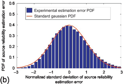

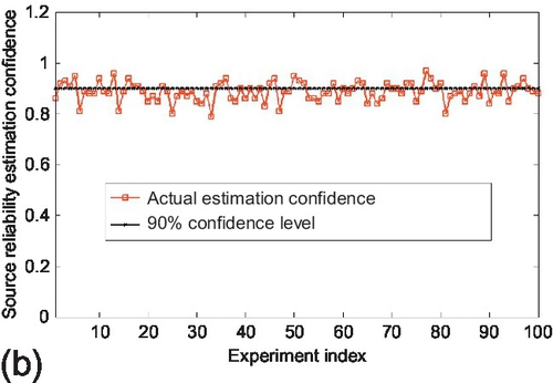
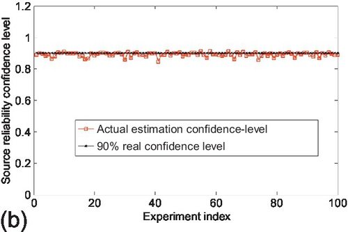
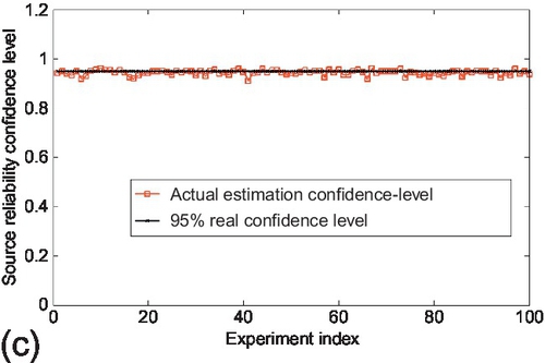
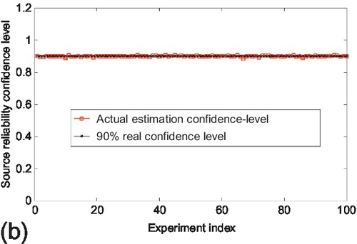
Figure 6.2 shows the comparison between the actual estimation confidence and three different confidence levels that were set for the small observation matrix scenario. The actual estimation confidence is computed as the percentage of sources whose estimation error stay within the corresponding confidence bound for every experiment. This percentage represents the probability that a randomly chosen source keeps its reliability estimation error within the confidence bound. We observe that the actual estimation confidence of using three different confidence bounds stays close to the corresponding confidence levels that were used for the experiment. Moreover, at higher confidence levels, a lower fluctuation of the actual estimation confidence is observed. Similar results are observed for the medium and large observation matrices as well, which are shown in Figures 6.3 and 6.4, respectively. Additionally, we also note that the fluctuation of the actual estimation confidence decreases as the observation matrix scale increases. This is because the estimation variance characterized by CRLB is inversely proportional to the number of claims in the system, which will be further evaluated in the next subsection.


6.5.2 Evaluation of CRLB
In this subsection, we review the evaluation of the accuracy of derived CRLBs (both actual and asymptotic) in Sections 6.2 and 6.3 by comparing them to the actual estimation variance of the estimation parameter (i.e., ai, bi). The actual estimation variance is characterized by the average RMSE (square root of the mean squared error) of all sources.
Scalability study
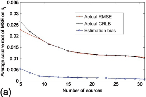
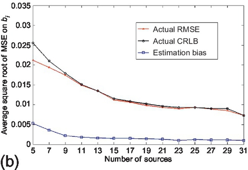
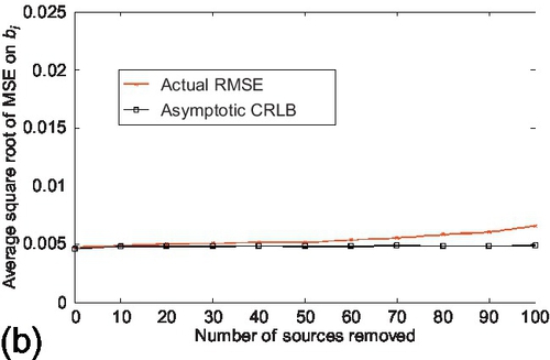
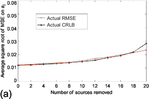
The scalability of CRLB performance with respect to the sensing topology (i.e., M and N) was first evaluated. The first experiment evaluates the effect of the number of sources (i.e., M) in the system on the CRLB performance. It started with the actual CRLB evaluation. The true and false claims were fixed to 1000 respectively, the average observations per source is set to 100. The number of sources from was varied 5 to 31. Reported results are averaged over 100 experiments and are shown in Figure 6.5. Observe that the actual CRLB tracks the variance of estimation parameters accurately even when the number of sources is small (e.g., M ≤ 20) in the system. We also observe that the RMSE is smaller than the actual CRLB when there are too few sources. This is because the MLE is biased on those points due to the small dataset. As illustrated in Section 6.2, the computation of actual CRLB does not scale with the number of sources in the system. Hence, the accuracy of asymptotic CRLB was also evaluated when the number of sources becomes large. The experimental configuration was kept the same as above, but the number of sources was changed from 10 to 150. Results are shown in Figure 6.6. We observe that the asymptotic CRLB deviates from the actual estimation variance when the number of sources is small (e.g., M ≤ 20). However, as the number of sources becomes sufficient in the network, the RMSE converges to the asymptotic CRLB quickly and the difference between the two becomes insignificant.


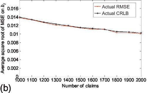
The second experiment compares the derived CRLBs (both actual and asymptotic) to the RMSE of estimation parameters when the number of claims (i.e., N) changes. As shown in Sections 6.2 and 6.3, both the actual and asymptotic CRLB decrease as 1N![]() . As before, the accuracy of actual CRLB was first evaluated. The number of sources was fixed as 20, the average number of observations per source is set to 100. The number of true and false claims were kept the same. The number of claims varies from 1000 to 2000. Reported results are averaged over 100 experiments and are shown in Figure 6.7. We observe that the actual CRLB is able to track the RMSE on estimation parameter correctly and they both decrease approximately as 1N
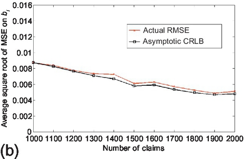
. As before, the accuracy of actual CRLB was first evaluated. The number of sources was fixed as 20, the average number of observations per source is set to 100. The number of true and false claims were kept the same. The number of claims varies from 1000 to 2000. Reported results are averaged over 100 experiments and are shown in Figure 6.7. We observe that the actual CRLB is able to track the RMSE on estimation parameter correctly and they both decrease approximately as 1N![]() when the number of claim increases. Similarly, the experiment was carried out to evaluate the accuracy of asymptotic CRLB. The experimental configuration was kept the same as above, but the number of sources was set to be 100. Results are shown in Figure 6.8. We observe that the asymptotic CRLB also follows closely on the RMSE of the estimation parameter and they reduce approximately as 1N
when the number of claim increases. Similarly, the experiment was carried out to evaluate the accuracy of asymptotic CRLB. The experimental configuration was kept the same as above, but the number of sources was set to be 100. Results are shown in Figure 6.8. We observe that the asymptotic CRLB also follows closely on the RMSE of the estimation parameter and they reduce approximately as 1N![]() when the number of claim increases.
when the number of claim increases.


Trustworthiness and assertiveness study
In the trustworthiness study, the estimation performance of CRLB was evaluated when the ratio of trusted sources in the system changes. The trusted sources are the sources who always make correct observations (i.e., their reliability is 1) and the ratio of trusted sources is the ratio of the number of trusted sources over the total number of sources in the system. The reliability of non-trusted sources is uniformly distributed in the range of (0,1). The true and false claims were fixed to 1000 respectively, the number of sources is set to 20 and each source reports 100 observations on average. The trusted source ratio was varied from 0 to 0.9. Reported results are averaged over 100 experiments and shown in Figure 6.9. Observe that the actual CRLB tracks the estimation variance tightly when the trusted source ratio changes. We also note that both the actual CRLB and the estimation variance of estimation parameters improve as the trusted source ratio increases. The reason is: the estimation error decreases as the ratio of sources with ti = 1 increases. This is also reflected by the fact that bi = 0 for trusted sources and the asymptotic variance goes to zero as one can see in (6.16). Similarly, experiments were carried out to evaluate the accuracy of the asymptotic CRLB. The experiment configuration was kept the same as above, but the number of sources was set to be 100. Results are shown in Figure 6.10. We observe that the asymptotic CRLB also follows the estimation variance of the estimation parameters correctly and they improve as the trusted source ratio increases.


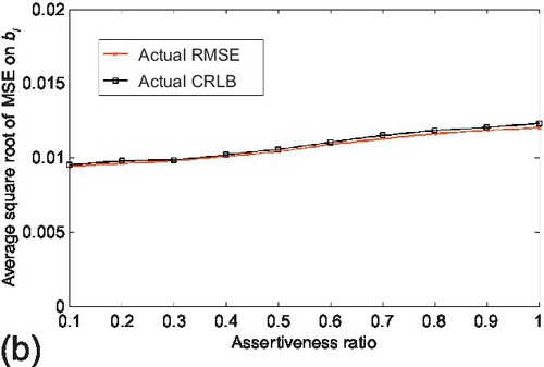
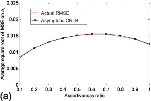
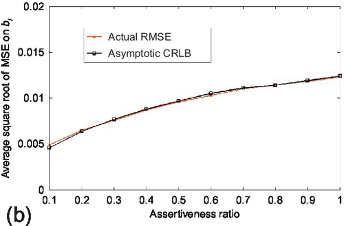
In the assertiveness study, the estimation performance of CRLB was evaluated when the assertiveness ratio of sources changes. The assertiveness ratio is defined as the ratio of the input data size (in terms of the number of observations) normalized by a pre-defined data size. This ratio reflects the sparsity of the sensing topology when the algorithm starts to run. The true and false claims were fixed to 1000 respectively. The number of sources is set to 20. The input data size that is used for the assertiveness ratio normalization (i.e., having assertiveness ratio of 1) is set to 1000 observations per source. The assertiveness ratio was varied from 0.1 to 1. Reported results are averaged over 100 experiments and shown in Figure 6.11. We observe that the actual CRLB tracks the RMSE of the estimation parameters correctly as the assertiveness ratio changes. We also note that the estimation variance of parameter ai first increases and then decreases while the estimation variance of parameter bi increases as the assertiveness ratio increases. The reason is: two factors affect the variance of the estimation parameters in different directions when the assertiveness ratio changes. One factor is the probability that a source reports a claim (i.e., si), defined in Section 6.1. This factor increases as the assertiveness ratio increases, which will enlarge the estimation variance of ai and bi based on (5.5). The other factor is the estimation variance of the source reliability (i.e., ti), which decreases as the assertiveness ratio increases. Hence, the estimation variance of ai is first dominated by the first factor and then by the second one while the estimation variance of bi is dominated by the first factor in the evaluation range as the assertiveness ratio increases. Similar experiments were then carried out to evaluate the accuracy of the asymptotic CRLB. The experiment configuration was kept the same as above, but the number of sources was set to be 100. Results are shown in Figure 6.12. We observe that the asymptotic CRLB also follows the variance of the estimation parameters tightly and their trends are similar as those of actual CRLB.

Robustness study
In the robustness study, the robustness (or sensitivity) of the estimation performance and the derived CRLBs were evaluated when the number of sources changes under different source reliability distributions. The key characteristic that determines the resilience of a network is the network topology. The social sensing topology is characterized by the link connections between sources and two sets of claims (i.e., true and false). The link connection skew is mainly determined by the source reliability distribution. Two representative network topologies were considered: scale-free and exponential topologies in the evaluation. For scale-free topology, sources have diverse reliability and the probability for sources to have different reliability is similar. For exponential topology, sources have similar reliability and nodes with higher reliability are exponentially less probable. The experiments were done by source removal (i.e., sources are randomly selected and removed from the system). This represents the scenario where random sources decide to quit the sensing application or their sensing devices fail. However, it is equivalent to reversing the steps and investigating the addition of sources.
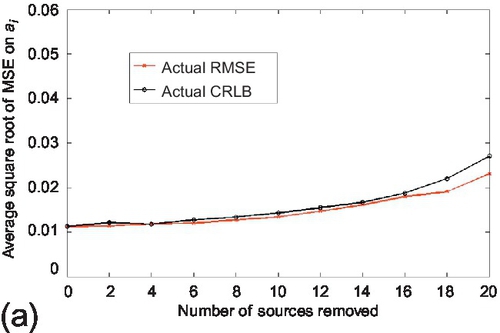
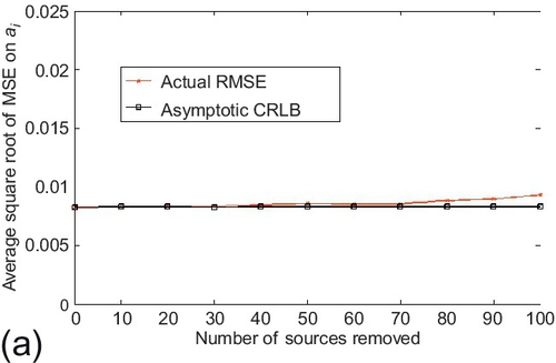
In the first experiment, the estimation performance and the derived CRLBs were evaluated under the scale-free network topology. To generate the scale-free network topology, source reliability follows a uniform distribution on its definition range. The actual CRLB compared to the RMSE on the estimation parameter. Both the number of true and false claims were fixed to 1000. The average number of observations per source was set to 100. The experiments started with 25 sources and gradually removed sources from the system. Figure 6.13 shows the actual CRLB and RMSE of the estimation parameter. Observe that the estimation accuracy (i.e., RMSE) degrades gracefully and the actual CRLB tracks the RMSE reasonably well as the number of removed sources increases. Also note that the actual CRLB deviates slightly from the RMSE when majority of sources are removed from the system. Then similar experiments were repeated for the asymptotic CRLB as well. The experiments started with 150 sources and gradually removed the sources from the system. Results are shown in Figure 6.14. The results for asymptotic CRLB are similar to actual CRLB.

In the second experiment, the estimation performance and the derived CRLBs were evaluated under the exponential network topology. To generate the exponential network topology, the source reliability follows a normal distribution (with the mean value as the mean of its definition range and a reasonably small variance). Similar as before, the actual CRLB compared to the RMSE on the estimation parameter. The standard deviation of the normal distribution of source reliability was set to 0.02, other settings were kept the same as the first experiment. Figure 6.15 shows the actual CRLB and RMSE of the estimation parameter. Observe that RMSE increases gradually as the number of removed sources grows and the actual CRLB tracks the RMSE well. Similar experiments were repeated for the asymptotic CRLB as well. The experimental settings were kept the same as the first experiment. Results are shown in Figure 6.16. Similar results of the actual CRLB are observed for the asymptotic CRLB.


For both the scale-free and exponential topology of social sensing, the above results show that the estimation performance is relatively robust (or insensitive) to changes in the number of sources in the network. Both actual and asymptotic CRLBs are able to track the estimation performance as long as a limited number of sources stay in the system.
6.5.3 Evaluation of Estimated False Positives/Negatives on Claim Classification
In this subsection, the estimated false positives/negatives on claim classification were evaluated by comparing them to the actual false positives/negatives (i.e., the ones that are computed from the ground truth). Similar experiments in the previous subsection were carried out to evaluate its performance through scalability, trustworthiness, assertiveness, and robustness studies.
Scalability study
The scalability of the estimated false positives/negatives with respect to the sensing topology were first evaluated. The first experiment evaluated the performance when the number of sources (i.e., M) in the system changes. The number of true and false claims were fixed to 1000 respectively, the average number of observations per source was set to 200. The number of sources was varied from 10 to 150. Reported results were averaged over 100 experiments and are shown in Figure 6.17. Observe that both estimated false positives and false negatives track the actual values accurately as the number of sources changes. We also note that the false positives/negatives decrease as the number of sources increases. The second experiment compared the estimated false positives/negatives to the actual values when the number of claims (i.e., N) changes. The number of sources was fixed as 50, the average number of observations per source was set to 200. The number of true and false claims as kept the same. The number of claims was varied from 1000 to 2000. Reported results are averaged over 100 experiments and shown in Figure 6.18. Observe that the estimated false positives/negatives are able to track the actual values correctly when the number of claims changes. We also note that the estimation performance degrades as the number of claims increases. The reason is: the sensing topology becomes sparser as the number of claims increases while the number of sources and observations per source stay the same.


Trustworthiness and assertiveness study
In the trustworthiness study, the estimated false positives/negatives were evaluated when the ratio of trusted sources changes in the system. In the experiment, the number of sources was set to be 50. The number of true and false claims were set to be 1000 respectively and the observations per source is set to be 200. The trusted source ratio was varied from 0 to 0.9. The reliability of non-trusted sources is uniformly distributed in the range of (0,1). The reported results are averaged over 100 experiments and shown in Figure 6.19. Observe that the estimated false positives/negatives track the actual values correctly and both of them decrease as the trusted source ratio increases. The reason is: trusted sources always provide correct observations, which helps the algorithm to estimate the truthfulness of claims more accurately.


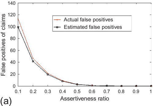
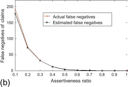
In the assertiveness study, the estimated false positives/negatives were evaluated when the assertiveness ratio changes in the system. In the experiment, the number of sources was fixed to be 50. The number of true and false claims were set to be 1000 respectively. The data size that is used for the assertiveness ratio normalization was set to 1000 observations per source. The assertiveness ratio was varied from 0.1 to 1. The reported results are averaged over 100 experiments and shown in Figure 6.20. Observe that the estimated false positives/negatives track the actual values correctly and both of them decrease as the assertiveness ratio increases. The reason is: the sensing topology becomes more densely connected and offers a better chance for the algorithm to correctly judge the truthfulness of the claims as the assertiveness ratio increases.
Robustness study
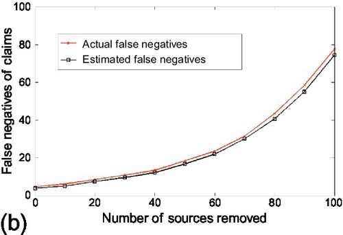
In the robustness study, similarly as before, the estimated false positives/negatives were evaluated when the number of sources changes under different source reliability distribution.† The first experiment evaluated the estimation performance of the scale-free network topology. The number of true and false claims were fixed to 1000. The average number of observations per source was set to 200. The experiment started with 150 sources and gradually removed sources from the system. Reported results are averaged over 100 experiments and shown in Figure 6.21. Observe that the estimation performance degrades and the estimated false positives/negatives track the actual values reasonably well as the number of removed sources increases. Also note that the estimated values deviate slightly from the actual values when majority of the sources are removed from the system. In the second experiment, the estimation performance was evaluated under the exponential network topology. The source reliability distribution was changed to be normal distribution and other settings were kept the same as the first experiment. Reported results are averaged over 100 experiments and shown in Figure 6.22. We observe the estimated false positives/negatives track the actual values well when a reasonable number of sources stay in the system. However, we also note that the estimation performance degrades compared to the results of scale-free topology. The reason is: sources are more likely to have similar reliability in the exponential topology. Such similarity makes it a more challenging scenario for the reviewed algorithm to accurately pinpoint the source reliability and identity the correctness of claims. For both scale-free and exponential topology, the above results show that the estimated false positives/negatives are able to track the actual values as long as limited number of sources stay in the system. The estimation performance on claim classification is relatively robust to changes in the number of sources in the network.


6.5.4 A Real World Case Study
In this section, we review the evaluation of the performance of the credibility estimation and confidence quantification approach through a real-world social sensing application. The goal of this application is to identify the correct locations of traffic lights and stop signs in the twin city of Urbana-Champaign by leveraging GPS devices on a set of vehicles traveling regularly in town. (The identified traffic light and stop sign locations were then used along with other information to compute fuel and delay estimates on city routes for a recent green navigation service [113]). The dataset from a smartphone-based vehicular sensing testbed, called SmartRoad [114] was used. Their test application, on the phone, recorded GPS traces, where every GPS reading is composed of an instantaneous latitude-longitude location, speed, time, and bearing of the vehicle. The application then computed simple features that constitute (intentionally unreliable) indicators that the vehicle is waiting at stop sign or a traffic light. Specifically, if a vehicle stops at a location for 15-90 s, the application concludes that it is stopped at a traffic light at that location. Similarly if it stops for 2-10 s, it concludes that it is at a stop sign. These conclusions were reported as claims from the corresponding source. The claim would be that a stop sign (or a traffic light, as applicable) exists at the current location and bearing. Clearly, these generated claims are unreliable, due to the simple-minded nature of the “sensor” and the complexity of road conditions and driver’s behaviors. For example, a car can stop anywhere on the road due to a traffic jam or a crossing pedestrian, not necessarily at the location of traffic lights or stop signs. Also, cars do not stop at traffic lights when they are green. Finally, different drivers have different attitudes toward stop signs. Some are more careless and may pass stop signs without stopping or do a “rolling stop,” whereas others reliably stop at each sign.
The general lack of reliability of claims and sources (and the differences in driver behavior) constituted a good test for the fact-finding algorithm described in this paper. Hence, the credibility estimation approach was applied to the collected claim data with the hope to find the correct locations of traffic lights and stop signs, and to identify the reliability of sources. For evaluation purposes, they also independently manually collected ground truth locations of traffic lights and stop signs.
In the experiment, 34 people were invited to participate in the application and 1,048,572 GPS readings (around 300 h of driving) were collected. A total of 4865 claims were generated by the phones, of which 3303 were for stop signs and 1562 were for traffic lights, collectively identifying 369 distinct locations. The observation matrix was generated by taking the sources as sources and their stop sign/traffic light reports as claims. The reviewed credibility estimation approach was applied to the data collected and its accuracy was evaluated at inferring which reports were correct.
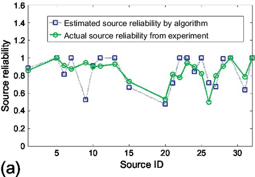
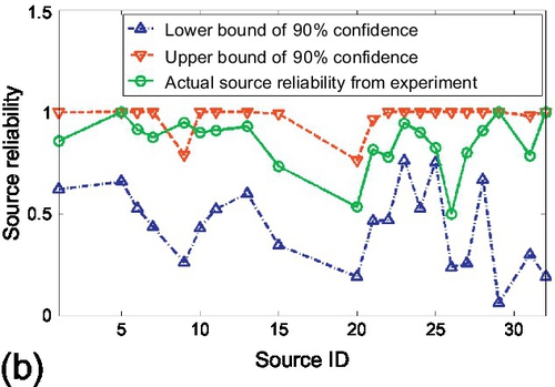
Figures 6.23 and 6.24 show the results for the case of traffic lights identification. Figure 6.23 shows the results of source reliability. In Figure 9.1, the source reliability estimated by the credibility estimation algorithm was compared with the actual source reliability (i.e., the percentage of claims from that source that were actually correct) computed from ground truth. We observed that estimated values track actual results well for most of the sources. Figure 6.23 (b) shows the 90% confidence bounds on source reliability estimation. We observe that actual source reliability stays mostly within the 90% confidence bound. Only 3 sources out of 34 (about 10%) have their reliability slightly outside the bound, which is what a 90% confidence interval means. Hence, the experiment verifies the accuracy and tightness of the confidence bounds derived in Section 6.4. The 68% and 95% confidence bounds were also examined and we observed that they capture the 70.6% and 94.1% of sources whose reliability estimations stay within bounds, respectively. This again verifies accuracy of those confidence intervals. Figure 6.24 shows the results of claim classification on traffic lights. All locations were sorted, where the system identified traffic lights (i.e., concluded that the corresponding claims were true), by the probability of correctness, also returned by the system. It is expected that traffic light locations identified with a higher probability will tend to be real lights, whereas those identified with a lower probability will include progressively more false positives.
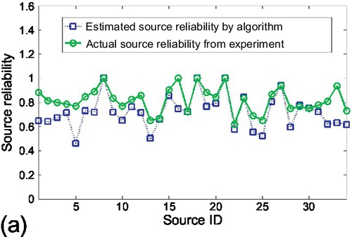
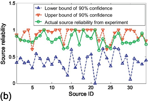

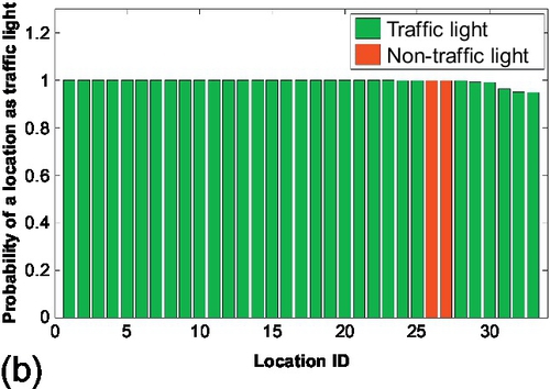
Figure 6.24 (a) shows the sorted locations on the x-axis, and computes for each n, the average probability that the first n locations are traffic lights. The estimated probability was compared to the actual ground truth probability. We observe that the estimation follows quite well the actual experimental ground truth. It verifies the accuracy of the probability values computed and used for claim classification. Additionally, Figure 6.24 (b) shows for each traffic light, in the same sorted order, the actual location status (i.e., whether a traffic light is in fact present at the location or not). We observe that most of the traffic light locations identified by the reviewed scheme are correct, although false positives arise as we go down in location ranking. The blue curve (dark gray in print versions) did have a slightly dip when false positives appear even though it is not very obvious in the figure.
The above experiments were repeated for stop sign identification and observed similar trends as in the case of traffic lights. However, the identification of stop signs is found to be more challenging than that of traffic lights. The reasons are: (i) the corroborated data for stop signs is sparser because the chances of different cars to stop at the same stop sign are much lower than that for traffic lights; (ii) cars have quite a few short wait behaviors at non-stop sign locations such as exists from parking lots, left turns, and pedestrian crossings; (iii) cars’ bearings are usually not well aligned with the directions of stop signs, which is especially true when the car wants to make a turn after the stop sign. Therefore, for the evaluation of stop signs, only sources whose reliability was more than 50% were picked. Figure 6.25 shows the estimation results of source reliability. We observe that the actual source reliability is estimated accurately and bounded correctly by the 90% confidence bounds. Figure 6.26 shows the results of claim classification at stop signs. We observe that the actual probability of correctness curve stays close to but slightly lower than the estimated one. The reasons of such deviation can be explained by the short wait behaviors mentioned above at non-stop sign locations in real world scenarios. In a sense, given the wait-based features, the reviewed algorithms actually did a better job at identifying actual stop locations of vehicles than would be predicted by looking at stop signs only. For example, it also found exits from parking lots and locations of pedestrian crossings. Note that, the aforementioned false positives gradually appear at locations that are ranked lower by the algorithm.


6.6 Discussion
This chapter reviews the derivation and evaluation of confidence intervals in source reliability and estimated classification accuracy of claims in social sensing. Some limitations exist in the reviewed work that offer opportunities for future work.
As we discussed in this chapter, the computation of actual CRLBs of the MLE is exponential with respect to the number of sources in the system. To resolve such computational limitation, the asymptotic CRLBs were also derived when there are enough sources and the correctness of claims can be estimated with full accuracy. However, there might exist a gap between the working ranges of two CRLBs in terms of the number of sources. For example, the number of sources in an application might be too large to efficiently compute actual CRLBs but too small for the asymptotic CRLBs to converge. Therefore, it would be interesting to develop new approximation algorithms to fill in the gap by efficiently computing the actual CRLBs or adjusting the asymptotic CRLBs to better track the estimation variance. We also note that the parameter d is also estimated in the EM scheme presented in Chapter 5. The future work could expand the computation of CRLB by including d in the calculation. Technically, this makes the actual CRLB calculation slightly more complicated, but it should have no effect on the asymptotic CRLB as the zj for each claim was assumed to be known in that case.
This chapter reviews recently developed confidence bounds on source reliability estimation error as well as estimated classification accuracy of claims in social sensing applications. The reviewed work allow the applications to not only assess the reliability of sources and claims, given neither in advance, but also estimate the accuracy of such assessment. The confidence bounds are computed based on the CRLB of the MLE of source reliability. The accuracy of claim classification is estimated by computing the probability that each claim is correct. The derived accuracy results are shown to predict actual errors very well. The results reviewed in this chapter are important because they allow social sensing applications to assess the reliability of un-vetted sources (like human sources) to a desired confidence level and estimate the accuracy of claim classification under the maximum likelihood hypothesis, in the absence of independent means to verify the data and in the absence of prior knowledge of reliability of sources. This is attained via a well-founded analytic problem formulation and a solution that leverages well-known results in estimation theory.
Appendix
The expectation term in Equation (6.7) can be further simplified:
E[(2Xkj−1)Zj(2Xlq−1)ZqaXkjk(1−ak)(1−Xkj)aXlql(1−al)(1−Xlq)]=∑x∈X(2Xkj−1)Zj(2Xlq−1)ZqaXkjk(1−ak)(1−Xkj)aXlql(1−al)(1−Xlq)p(X|θ)=∑x∈X(2Xkj−1)(2Xlq−1)ZjZqaXkjk(1−ak)(1−Xkj)aXlql(1−al)(1−Xlq)×(∏Nj′=1{∏Mi=1aXij′i(1−ai)(1−Xij′)×d+∏Mi=1bXij′i(1−bi)(1−Xij′)×(1−d)})
When j≠q, plugging the expressions of Zj and Zq, the expectation term in Equation (6.7) is shown to be zero:
E[(2Xkj−1)Zj(2Xlq−1)ZqaXkjk(1−ak)(1−Xkj)aXlql(1−al)(1−Xlq)]=∑x∈X(2Xkj−1)(2Xlq−1)×(∏Mi=1i≠kaXiji(1−ai)(1−Xij)×d∏Mi=1i≠laXiqi(1−ai)(1−Xiq)×d)×(∏Nj′=1j′≠jorq{∏Mi=1aXij′i(1−ai)(1−Xij′)×d+∏Mi=1bXij′i(1−bi)(1−Xij′)×(1−d)})=∑x∈Xj×Xq(2Xkj−1)(2Xlq−1)×(∏Mi=1i≠kaXiji(1−ai)(1−Xij)×d∏Mi=1i≠laXiqi(1−ai)(1−Xiq)×d)=(∏Mi=1i≠kaXiji(1−ai)(1−Xij)×d∏Mi=1i≠laXiqi(1−ai)(1−Xiq)×d)×∑1Xkj=0∑1Xlq=0(2Xkj−1)(2Xlq−1)=0j≠q
