5.2.1 Background

The EM algorithm is useful when the likelihood expression simplifies by the inclusion of a latent variable. Considering a latent variable Z, the likelihood function is given by:

$\begin{array}{l}\hfill L(\theta ;X)=p(X|\theta )=\sum _{Z}p(X,Z|\theta )\end{array}$

where p(X,Z|θ) is L(θ|X,Z), which is uni-modal and easy to solve.

Once the formulation is complete, the EM algorithm finds the MLE by iteratively performing the following steps:

• E-step: Compute the expected log likelihood function where the expectation is taken with respect to the computed conditional distribution of the latent variables given the current settings and observed data.

$\begin{array}{l}\hfill Q(\theta |{\theta }^{(t)})=E_{Z|X,{\theta }^{(t)}}[logL(\theta ;X,Z)]\end{array}$

• M-step: Find the parameters that maximize the Q function in the E-step to be used as the estimate of θ for the next iteration.

$\begin{array}{l}\hfill {\theta }^{(t+1)}=\underset{\theta }{argmax}Q(\theta |{\theta }^{(t)})\end{array}$

5.2.2 Mathematical Formulation

The social sensing problem fits nicely into the EM model. First, a latent variable Z is introduced for each claim to indicate whether it is true or not. Specifically, a corresponding variable z_j is defined for the jth claim C_j such that: z_j = 1 when C_j is true and z_j = 0 otherwise. The observation matrix SC is denoted as the observed data X, and θ = (a₁,a₂,…,a_M;b₁,b₂,…,b_M;d) is defined as the parameter of the model that needs to be estimated. The goal is to obtain the MLE of θ for the model containing observed data X and latent variables Z.

The likelihood function L(θ;X,Z) is given by:

$\begin{array}{ll}\hfill L(\theta ;X,Z)& =p(X,Z|\theta )\hfill \\ \hfill & =\prod _{j=1}^N\left\{\prod _{i=1}^M{a}_i^{S_i{C}_j}{(1-a_i)}^{(1-S_i{C}_j)}\times d\times z_j\right.\hfill \\ \hfill & +\left.\prod _{i=1}^M{b}_i^{S_i{C}_j}{(1-b_i)}^{(1-S_i{C}_j)}\times (1-d)\times (1-z_j)\right\}\hfill \end{array}$

where, as we mentioned before, a_i and b_i are the conditional probabilities that source S_i reports the claim C_j to be true given that C_j is true or false (i.e., defined in Equation (5.2)). S_iC_j = 1 when source S_i reports that C_j is true, and S_iC_j = 0 otherwise. d is the background bias that a randomly chosen claim is true. Additionally, it is assumed that sources and claims are independent respectively. The likelihood function above describes the likelihood to have current observation matrix X and hidden variable Z given the estimation parameter θ.

5.2.3 Deriving the E-Step and M-Step

Given the above formulation, substitute the likelihood function defined in Equation (5.10) into the definition of Q function given by Equation (5.8) of EM. The Expectation step (E-step) becomes:

$\begin{array}{ll}\hfill Q(\theta |{\theta }^{(t)})& =E_{Z|X,{\theta }^{(t)}}[logL(\theta ;X,Z)]\hfill \\ \hfill & =\sum _{j=1}^N\left\{p(z_j=1|X_j,{\theta }^{(t)})\right.\hfill \\ \hfill & \times \left[\sum _{i=1}^M(S_i{C}_{j}log{a}_i+(1-S_i{C}_j)log(1-a_i)+logd)\right]+p(z_j=0|X_j,{\theta }^{(t)})\hfill \\ \hfill & \left.\times \left[\sum _{i=1}^M(S_i{C}_{j}log{b}_i+(1-S_i{C}_j)log(1-b_i)+log(1-d))\right]\right\}\hfill \end{array}$

where X_j represents the jth column of the observed SC matrix (i.e., observations of the jth claim from all sources) and p(z_j = 1|X_j,θ^(t)) is the conditional probability of the latent variable z_j to be true given the observation matrix related to the jth claim and current estimate of θ, which is given by:

$\begin{array}{ll}\hfill p(z_j=1|X_j,{\theta }^{(t)})& =\frac{p(z_j=1;X_j,{\theta }^{(t)})}{p(X_j,{\theta }^{(t)})}\hfill \\ \hfill & =\frac{p(X_j,{\theta }^{(t)}|z_j=1)p(z_j=1)}{p(X_j,{\theta }^{(t)}|z_j=1)p(z_j=1)+p(X_j,{\theta }^{(t)}|z_j=0)p(z_j=0)}\hfill \\ \hfill & =\frac{A(t,j)\times d^{(t)}}{A(t,j)\times d^{(t)}+B(t,j)\times (1-d^{(t)})}\hfill \end{array}$

where A(t,j) and B(t,j) are defined as:

$\begin{array}{ll}\hfill A(t,j)& =p(X_j,{\theta }^{(t)}|z_j=1)\hfill \\ \hfill & =\prod _{i=1}^M{a}_i^{(t)S_i{C}_j}{(1-a_i^{(t)})}^{(1-S_i{C}_j)}\hfill \\ \hfill B(t,j)& =p(X_j,{\theta }^{(t)}|z_j=0)\hfill \\ \hfill & =\prod _{i=1}^M{b}_i^{(t)S_i{C}_j}{(1-b_i^{(t)})}^{(1-S_i{C}_j)}\hfill \end{array}$

A(t,j) and B(t,j) represent the conditional probability regarding observations about the jth claim and current estimation of the parameter θ given the jth claim is true or false, respectively.

Next Equation (5.11) is simplified by noting that the conditional probability of p(z_j = 1|X_j,θ^(t)) given by Equation (5.12) is only a function of t and j. Thus, it is represented by Z(t,j). Similarly, p(z_j = 0|X_j,θ^(t)) is simply:

$\begin{array}{ll}\hfill p(z_j=0|X_j,{\theta }^{(t)})& =1-p(z_j=1|X_j,{\theta }^{(t)})\hfill \\ \hfill & =\frac{B(t,j)\times (1-d^{(t)})}{A(t,j)\times d^{(t)}+B(t,j)\times (1-d^{(t)})}\hfill \\ \hfill & =1-Z(t,j)\hfill \end{array}$

Substituting from Equations (5.12) and 5.14 into Equation (5.11), we get:

$\begin{array}{ll}\hfill Q(\theta |{\theta }^{(t)})& =\sum _{j=1}^N\left\{Z(t,j)\times \left[\sum _{i=1}^M(S_i{C}_{j}log{a}_i+(1-S_i{C}_j)log(1-a_i)+logd)\right]\right.\hfill \\ \hfill & \left.+(1-Z(t,j))\times \left[\sum _{i=1}^M(S_i{C}_{j}log{b}_i+(1-S_i{C}_j)log(1-b_i)+log(1-d))\right]\right\}\hfill \end{array}$

The Maximization step (M-step) is given by Equation (5.9). θ* (i.e., $(a_1^{*},a_2^{*},\dots ,a_M^{*};b_1^{*},b_2^{*},\dots ,b_M^{*};d^{*})$) is chosen to maximize the Q(θ|θ^(t)) function in each iteration to be the θ^(t+1) of the next iteration.

To get θ* that maximizes Q(θ|θ^(t)), the derivatives are set to 0: $\frac{\partial Q}{\partial a_i}=0$, $\frac{\partial Q}{\partial b_i}=0$, $\frac{\partial Q}{\partial d}=0$ which yields:

$\begin{array}{ll}\hfill \sum _{j=1}^N\left[Z(t,j)\left(S_i{C}_j\frac{1}{a_i^{*}}-(1-S_i{C}_j)\frac{1}{1-a_i^{*}}\right)\right]& =0\hfill \\ \hfill \sum _{j=1}^N\left[(1-Z(t,j))\left(S_i{C}_j\frac{1}{b_i^{*}}-(1-S_i{C}_j)\frac{1}{1-b_i^{*}}\right)\right]& =0\hfill \\ \hfill \sum _{j=1}^N\left[Z(t,j)M\frac{1}{d^{*}}-(1-Z(t,j))M\frac{1}{1-d^{*}}\right]& =0\hfill \end{array}$

Let us define SJ_i as the set of claims the source S_i actually observes in the observation matrix SC, and $\overline{S{J}_i}$ as the set of claims source S_i does not observe. Thus, Equation (5.16) can be rewritten as:

$\begin{array}{ll}\hfill \sum _{j\in S{J}_i}Z(t,j)\frac{1}{a_i^{*}}-\sum _{j\in \overline{S{J}_i}}Z(t,j)\frac{1}{1-a_i^{*}}& =0\hfill \\ \hfill \sum _{j\in S{J}_i}(1-Z(t,j))\frac{1}{b_i^{*}}-\sum _{j\in \overline{S{J}_i}}(1-Z(t,j))\frac{1}{1-b_i^{*}}& =0\hfill \\ \hfill \sum _{j=1}^N\left[Z(t,j)\frac{1}{d^{*}}-(1-Z(t,j))\frac{1}{1-d^{*}}\right]& =0\hfill \end{array}$

Solving the above equations, the expressions of the optimal $a_i^{*}$, $b_i^{*}$, and d* are:

$\begin{array}{ll}\hfill a_i^{(t+1)}& =a_i^{*}=\frac{\sum _{j\in S{J}_i}Z(t,j)}{\sum _{j=1}^{N}Z(t,j)}\hfill \\ \hfill b_i^{(t+1)}& =b_i^{*}=\frac{K_i-\sum _{j\in S{J}_i}Z(t,j)}{N-\sum _{j=1}^{N}Z(t,j)}\hfill \\ \hfill d_i^{(t+1)}& =d_i^{*}=\frac{\sum _{j=1}^{N}Z(t,j)}{N}\hfill \end{array}$

where K_i is the number of claims espoused by source S_i and N is the total number of claims in the observation matrix.

Given the above, the E-step and M-step of EM optimization reduce to simply calculating Equations (5.12) and 5.18 iteratively until they converge. The convergence analysis has been done for EM scheme and it is beyond the scope of this chapter [108]. In practice, the algorithm runs until the difference of estimation parameter between consecutive iterations becomes insignificant. Since the claim is binary, the decision vector H* can be computed from the converged value of Z(t,j). Specially, h_j is true if Z(t,j) ≥ 0.5 and false otherwise. At the same time, the estimation vector E* of source reliability can also be computed from the converged values of $a_i^{(t)}$, $b_i^{(t)}$, and d^(t) based on their relationship given by Equation (5.5). This completes the mathematical development. The resulting algorithm is summarized in the subsection below.

5.4.1 A Simulation Study

The simulator as described in the previous chapter was used in the simulation study. Remember that, as stated in the application model, sources do not report “lack of problems.” Hence, they never report a variable to be false. Let t_i be uniformly distributed between 0.5 and 1 in the experiments. For initialization, the initial values of source reliability (i.e., t_i) in the evaluated schemes are set to the mean value of its definition range. The performance of EM scheme is compared to Bayesian interpretation [39] and three state-of-art fact-finder schemes from prior literature that can function using only the inputs offered in the reliable social sensing problem formulation [35–37]. Results show a significant performance improvement of EM over all heuristics compared.

The first experiment compares the estimation accuracy of EM and the baseline schemes by varying the number of sources in the system. The number of reported claims was fixed at 2000, of which 1000 variables were reported correctly and 1000 were misreported. To favor the competition, the other baseline algorithms were given the correct value of bias d (in this case, d = 0.5). The average number of observations per source was set to 100. The number of sources was varied from 20 to 110. Reported results are averaged over 100 random source reliability distributions. Results are shown in Figure 5.2. Observe that EM has the smallest estimation error on source reliability and the least false positives among all schemes under comparison. For false negatives, EM performs similarly to other schemes when the number of sources is small and starts to gain improvements when the number of sources becomes large. This is because sources are assumed to espouse more true claims than false ones and more sources will provide better evidence for the algorithm to correctly classify claims. Note also that the performance gain of EM becomes large when the number of sources is small, illustrating that EM is more useful when the observation matrix is sparse.

The second experiment compares EM with baseline schemes when the average number of observations per source changes. As before, the number of correctly and incorrectly reported variables was fixed to 1000 respectively. Again, the competition favored by giving the baseline algorithms the correct value of background bias d (here, d = 0.5). The number of sources was set to 30. The average number of observations per source is varied from 100 to 1000. Results are averaged over 100 experiments. The results are shown in Figure 5.3. Observe that EM outperforms all baselines in terms of both source reliability estimation accuracy and false positives as the average number of observations per source changes. For false negatives, EM has similar performance as other baselines when the average number of observations per source is small and starts to gain advantage as the average number of observations per source becomes large. This is because most observations are assumed to be true and more observations will provide better evidence for the algorithm to correctly classify claims. As before, the performance gain of EM is higher when the average number of observations per source is low, verifying once more the high accuracy of EM for sparser observation matrices.

The third experiment examines the effect of changing the claim mix on the estimation accuracy of all schemes. The ratio of the number of correctly reported variables to the total number of reported variables was varied from 0.1 to 0.6, while fixing the total number of such variables to 2000. To favor the competition, the background bias d is given correctly to the other algorithms (i.e., d = varying ratio). The number of sources is fixed at 30 and the average number of observations per source is set to 150. Results are averaged over 100 experiments. These results are shown in Figure 5.4. We observe that EM has almost the same performance as other fact-finder baselines when the fraction of correctly reported variables is relatively small. The reason is that the small amount of true claims are densely observed and most of them can be easily differentiated from the false ones by both EM and baseline fact-finders. However, as the number of variables (correctly) reported as true grows, EM is shown to have a better performance in both source reliability and claim estimation. Additionally, we also observe that the Bayesian interpretation scheme predicts less accurately than other heuristics under some conditions. This is because the estimated posterior probability of a source to be reliable or a claim to be true in Bayesian interpretation is a linear transform of source and claim credibility values. Those values obtained from a single or sparse observation matrix may not be very accurate and must be refined [39].

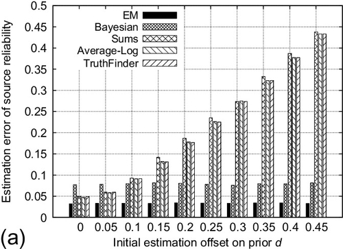
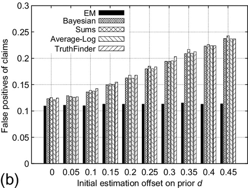
The fourth experiment evaluates the performance of EM and other schemes when the offset of the initial estimation on the background bias d varies. The offset is defined as the difference between initial estimation on d and its ground-truth. The number of correctly and incorrectly reported variables was set to 1000 respectively (i.e., d = 0.5). The absolute value of the initial estimate offset on d was varied from 0 to 0.45. The reported results are averaged for both positive and negative offsets of the same absolute value. The number of sources is fixed at 50 and the average number of observations per source is set to 150. Reported results are averaged over 100 experiments. Figure 5.5 shows the results. We observe that the performance of EM scheme is stable as the offset of initial estimate on d increases. On the contrary, the performance of other baselines degrades significantly when the initial estimate offset on d becomes large. This is because the EM scheme incorporates the d as part of its estimation parameter and provides the MLE on it. However, other baselines depend largely on the correct initial estimation on d (e.g., from the past history) to find out the right number of correctly reported claims. These results verify the robustness of the EM scheme when the accurate estimate on the prior d is not available to obtain.

The fifth experiment shows the convergence property of the EM iterative algorithm in terms of the estimation error on source reliability, as well as the false positives and false negatives on claims. The number of correctly and incorrectly reported variables was fixed to 1000 respectively and the initial estimate offset on d was set to 0.3. The number of sources is fixed at 50 and the average number of observations per source is set to 250. Reported results are averaged over 100 experiments. Figure 5.6 shows the results. We observe that both the estimation error on source reliability and false positives/negatives on claim converge reasonably fast (e.g., less than 10 iterations) to stable values as the number of iterations of EM algorithm increases. It verifies the efficiency of applying EM scheme to solve the MLE problem formulated. Note that the false negatives increase as the number of iteration increases. This is because the initial d was set to 0.8 which is larger than its true value (i.e., 0.5). Hence, the initial estimate of false negatives by the algorithm is smaller than its converged value (e.g., the algorithm could initially take true claims that very few sources reported as true and later classify them as false).

5.4.2 A Geotagging Case Study

In this subsection, we reviewed the application the EM scheme to a typical social sensing application: Geotagging locations of litter in a park or hiking area. In this application, litter may be found along the trails (usually proportionally to their popularity). Sources visiting the park geotag and report locations of litter. Their reports are not reliable however, erring both by missing some locations, as well as misrepresenting other objects as litter. The goal of the application is to find where litter is actually located in the park, while disregarding all false reports.

To evaluate the performance of different schemes, two metrics of interest were defined: (i) false negatives defined as the ratio of litter locations missed by a scheme to the total number of litter locations in the park, and (ii) false positives defined as the ratio of the number of incorrectly labeled locations by a scheme, to the total number of locations in the park. The EM scheme was compared to the Bayesian interpretation scheme and to voting, where locations are simply ranked by the number of times people report them.

A simplified trail map of a park represented by a binary tree was created and shown in Figure 5.7. The entrance of the park (e.g., where parking areas are usually located) is the root of the tree. Internal nodes of the tree represent forking of different trails. It is assumed trails are quantized into discretely labeled locations (e.g., numbered distance markers). In the emulation, at each forking location along the trails, sources have a certain probability P_c to continue walking and 1 − P_c to stop and return. Sources who decide to continue have equal probability to select the left or right path. The majority of sources are assumed to be reliable (i.e., when they geotag and report litter at a location, it is more likely than not that the litter exists at that location).

The first experiment studied the effect of the number of people visiting the park on the estimation accuracy of different schemes. A binary tree with a depth of 4 was chosen as the trail map of the park. Each segment of the trail (between two forking points) is quantized into 100 potential locations (leading to 1500 discrete locations in total on all trails). We define the pollution ratio of the park to be the ratio of the number of littered locations to the total number of locations in the park. The pollution ratio is fixed at 0.1 for the first experiment. The probability that people continue to walk past a fork in the path is set to be 95% and the percent of reliable sources is set to be 80%. The reliability of unreliable sources is uniformly distributed over (0,0.5). Reliable sources will report all pollution that they see. The number of sources visiting the park was varied from 5 to 50. The corresponding estimation results of different schemes are shown in Figure 5.8. Observe that both false negatives and false positives decrease as the number of sources increases for all schemes. This is intuitive: the chances of finding litter on different trails increase as the number of people visiting the park increases. Note that, the EM scheme outperforms others in terms of false negatives, which means EM can find more pieces of litter than other schemes under the same conditions. The improvement becomes significant (i.e., around 20%) when there is a sufficient number of people visiting the park. For the false positives, EM performs similarly to Bayesian interpretation and Truth Finder scheme and better than voting. Generally, voting performs the worst in accuracy because it simply counts the number of reports complaining about each location but ignores the reliability of individuals who make them.

The second experiment showed the effect of park pollution ratio (i.e., how littered the park is) on the estimation accuracy of different schemes. The number of individuals visiting the park is set to be 40. The pollution ratio of the park was varied from 0.05 to 0.15. The estimation results of different schemes are shown in Figure 5.9. Observe that both the false negatives and false positives of all schemes increase as the pollution ratio increases. The reason is that: litter is more frequently found and reported at trails that are near the entrance point. The amount of unreported litter at trails that are far from entrance increases more rapidly compared to the total amount of litter as the pollution ratio increases. Note that, the EM scheme continues to find more actual litter compared to other baselines. The performance of false positives is similar to other schemes.

The third experiment evaluated the effect of the initial estimation offset of the pollution ratio on the performance of different schemes. The pollution ratio is fixed at 0.1 and the number of individuals visiting the park is set to be 40. The absolute value of initial estimation offset of the pollution ratio was varied from 0 to 0.09. Results are averaged over both positive and negative offsets of the same absolute value. The estimation results of different schemes are shown in Figure 5.10. Observe that EM finds more actual litter locations and reports less falsely labeled locations than other baselines as the initial estimation offset of pollution ratio increases. Additionally, the performance of EM scheme is stable while the performance of other baselines drops substantially when the initial estimation offset of the pollution ratio becomes large.

The above evaluation demonstrates that the new EM scheme generally outperforms the current state of the art in inferring facts from social sensing data. This is because the state of the art heuristics infer the reliability of sources and correctness of facts based on the hypothesis that their relationship can be approximated linearly [36, 37, 39]. However, EM scheme makes its inference based on a maximum likelihood hypothesis that is most consistent with the observed sensing data, thus it provides an optimal solution.

5.4.3 A Real World Application

In this subsection, we reviewed the evaluation of the performance of the EM scheme through a real-world social sensing application, based on Twitter. The objective was to see whether the EM scheme would distill from Twitter feeds important events that may be newsworthy and reported by media. Specifically, the news coverage of Hurricane Irene was followed and 10 important events reported by media during that time were manually selected as ground truth. Independently from that collection, more than 600,000 tweets originating from New York City during Hurricane Irene were obtained using the Twitter API (by specifying keywords as “hurricane,” “Irene,” and “flood”, and the location to be New York). These tweets were collected from August 26 until September 2nd, roughly when Irene struck the east coast. Retweets were removed from the collected data to keep sources as independent as possible.

An observation matrix was generated from these tweets by clustering them based on the Jaccard distance metric (a simple but commonly used distance metric for micro-blog data [110]). Each cluster was taken as a statement of claim about current conditions, hence representing a claim in the MLE model. Sources contributing to the cluster were connected to that variable forming the observation matrix. In the formed observation matrix, sources are the twitter users who provided tweets during the observation period, claims are represented by the clusters of tweets and the element S_iC_j is set to 1 if the tweets of source S_i belong to cluster C_j, or to 0 otherwise. The matrix was then fed to the EM scheme. The scheme ran on the collected data and picked the top (i.e., most credible) tweet in each hour. It was then checked if 10 “ground truth” events were reported among the top tweets. Table 5.3 compares the ground truth events to the corresponding top hourly tweets discovered by EM. The results show that indeed all events were reported correctly, demonstrating the value of EM scheme in distilling key information from large volumes of noisy data. Voting was observed to have similarly good performance in this case study. However, in other case studies, the EM scheme was shown to have a better coverage of events than the voting scheme [50].