4.1 Facts, Fact-Finders, and the Existence of Ground Truth

Fact-finders are an interesting class of algorithms whose purpose is to recognize “truth” from observations that are noisy, conflicting, and possibly incomplete. As such, they are quite fundamental to our quest to build reliable systems on unreliable data. The majority of fact-finders can be thought of as algorithms that combine two fundamental components, whose use is prevalent in data mining literature. Namely, fact-finders intertwine the use of clustering and ranking components. Informally, the clustering component combines together pieces of evidence in support of the same facts. The ranking component weights the trustworthiness, credibility, authority, or probability of correctness of different clusters of evidence. Different fact-finders vary in how they perform the ranking and clustering steps. While both ranking and clustering are well-researched areas in data mining, the fact-finding problem itself is a bit of a special case, because, unlike most other data mining problems, fact-finders typically deal with situations, where a unique externally defined ground truth exists.

To appreciate what the above statement means, let us first elaborate on what we mean by externally defined ground truth. This is a concept we inherit from sensing and data fusion, where the objective is always to estimate the state of some external system; the system being monitored. That system is assumed to have state that is independent of what the sensing and data fusion algorithms are doing. That state is unique and unambiguous. While the sensors may be noisy and the estimation algorithms might make simplifying assumptions about how the monitored system behaves, once an estimate of the state is obtained, this estimate can, in principle, be compared to a unique and unambiguous actual state. Any difference between the actual and estimated states would constitute a unique and unambiguous measure of estimation error.

Note that, many algorithms can define their own set of assumptions. Under this set of assumptions, they may reach optimal conclusions. While the algorithms may be optimal in that sense, they may or may not do well in terms of estimation error. It all depends on how well their simplifying assumptions approximate the real world.

Now, let us go back to our previous statement. We pointed out that the existence of a unique externally defined ground truth in fact-finding problems makes them different from many other clustering and ranking problems. Consider, for example, community detection. The goal is usually to identify different communities (clusters of nodes) based on node interaction patterns. The solution consists of the clusters that have been identified. It is generally hard to compare these clusters to a metric of ground truth. It could be, for example, that communities were split across belief boundaries, such as liberals versus conservatives. However, it is not straightforward to define what exactly constitutes a liberal and what exactly constitutes a conservative. Hence, it is hard to tell in an unambiguous way whether the resulting clusters are consistent with “ground truth” or not. In some sense, the formed clusters define their own ground truth. An optimal solution to a clustering problem simply says that according to the distance metric used for clustering, the resulting clusters are optimal and constitute the best answer to the problem.

The same lack of an externally defined ground truth can be said about many ranking problems as well, investigated in data mining literature. For example, recent work in data mining develops algorithms for combined ranking and clustering [86]. The algorithm is used to rank the top 10 conferences and the top 10 authors in several fields. The results are intuitive in that the best conferences and the most recognized authors indeed come on top. However, it is hard to define an objective measure of error because it is hard to quantify ground truth. After all, how would one define a top author? Is it the number of publications they have? Is it the number of citations to their work? Is it their success in technology transfer from published research? There is no single, unique, agreed-upon metric and therefore no single, unique, agreed-upon ground truth. The ranking algorithm defines its own ground truth based on some assumed model. For example, under the simplifying assumption that better authors have more papers, one can come up with a unique and unambiguous ranking. However, there is no unique external reference to compare this resulting ranking to in order to determine how accurate exactly the simplifying assumption underlying the ranking was. It is precisely the existence of an external reference (for what is considered “true”) versus the lack thereof that is the distinction we are trying to draw between problems for which an externally defined ground truth exists and problems for which it does not.

Now, by contrast, consider the problem of fact-finding. Let the goal of the fact-finder be to identify which of a set of facts claimed by some unreliable sources actually occurred in the physical world. The fact-finding algorithm can make simplifying assumptions about how sources behave. Based on those assumptions some answers are given. Once the answers are given, it is in principle possible to define an error based on a comparison of what the fact-finder believed and what was actually true in the external physical world. The distinction is important because it allows us to formulate fact-finding problems as ones of minimizing the difference between exact and estimated states of systems. In other words, we cast them as sensing problems and are thus able to apply results from traditional estimation theory.

It remains to make two more points clear. First, the assumption of the existence of an externally defined unique ground truth does not necessarily mean that this ground truth is available to the fact-finding algorithm. In fact, most of the time, it is not. By analogy with target tracking algorithms, when the position of a target is estimated, one can define the notion of an estimation error even if this error is not available in practice because the data fusion system does not know the exact location of the target. (After all, if it did, we would not need to do the estimation in the first place.) The point is that the target has a unique and unambiguous location in the physical world at any given time. The deviation of the estimate from that actual location is the error. Estimation theory quantifies bounds on that error under different conditions.

The second point is that the existence of ground truth versus lack thereof does not constitute an advantage of one set of problems or solutions over another. The discussion above simply sheds light on an interesting difference between many problems addressed in data mining and problems addressed in sensing. Philosophically speaking, data mining is about discovery of uncharted territory. Hence, by definition, no agreed upon models for ground truth need to exist. If anything, the goal is to discover what ground truth might be. Sensing, on the other hand, is about reconstruction of an existing physical world in cyberspace. Therefore, by definition, sensing is only as good as the accuracy to which it reconstructs world state, compared to ground truth. In this book, the problem addressed is fundamentally one of sensing, although it does use inspiration from data mining literature. We define a notion of error and set up the fact-finding problem as one of minimizing this error. First, however, we take a look at previous literature in the area.

4.2 Overview of Fact-Finders in Information Networks

In this section, we first review several state-of-the-art fact-finders used in information network analysis. Some early fact-finder models include Sums (Hubs and Authorities) [35], TruthFinder [36], Average Log, Investment, and Pooled Investment [37]. Sums developed a basic fact-finder where the belief in a claim c is $B^i(c)={\sum }_{s\in S_c}{T}^i(s)$ and the truthfulness of a source s is $T^i(s)={\sum }_{c\in C_s}{B}^{(i-1)}(c)$, where S_c and C_s are the sources asserting a given claim and the claims asserted by a particular source, respectively. Both B(c) and T(s) are normalized by dividing by the maximum values in the respective vector to prevent them from going unbounded. TruthFinder is the first unsupervised fact-finder proposed by Yin et al. for trust analysis on a providers-facts network [36]. It models the fact-finding problem as a graph estimation problem where three types of nodes in the graph represent providers (sources), facts (claims), and objects, respectively. They assumed multiple mutual exclusive facts are associated with an object and providers assert facts of different objects. The proposed algorithm iterates between the computation of trustworthiness of sources and confidence of claims using heuristic based pseudo-probabilistic methods. In particular, the algorithm computes the “probability” of a claim by assuming that each source’s trustworthiness is the probability of it being correct and then average claim beliefs to obtain trustworthiness scores. Pasternack et al. extended the Sums framework by incorporating prior knowledge into the analysis and proposed several extended algorithms: Average Log, Investment, and Pooled Investment [37]. Average Log attempts to address the trustworthiness overestimation problem of a source who makes relatively few claims by explicitly considering the number of claims in the trustworthiness score computation. In particular, it adjusts the update rule to compute source trustworthiness score used in Sums as $T^i(s)=log|C_s|\frac{{\sum }_{c\in C_s}{B}^{i-1}(c)}{|C_s|}$. In Investment and Pooled Investment, sources “invest” their trustworthiness uniformly among claims and a non-linear function G was introduced to model the belief growth in each claim. Other fact-finders further enhanced the above basic framework by incorporating analysis on properties or dependencies within claims or sources. Galland et al. [38] took the notion of hardness of facts into consideration and proposed their algorithms: Cosine, 2-Estimates, and 3-Estimates. Dong et al. studied the source dependency and copying problem comprehensively and proposed several algorithms that give higher credibility to independent sources [41, 42, 97].

More recent works came up with several new fact-finding algorithms toward building more generalized framework and using more rigorous statistic models. Pasternack et al. [44] provided a generalized fact-finder framework to incorporate the background knowledge such as the confidence of the information extractor, attributes of information sources and similarity between claims. Instead of considering the source claim network as an unweighted bipartite graph, they proposed a generalized k-partite weighted graph where different types of background knowledge and contextual details can be encoded as weight links. Specifically, they defined the uncertainty expressed by the source in the claim, the attributes of sources and similarity between claims as different weights in their lifted model. They also rewrote several basic fact-finders (e.g., Sums, Average Log, Investment, and TruthFinder) to incorporate the background knowledge as the link weights in the computation of source trustworthiness and claim beliefs. New “layers” of groups and attributes can be added to the source and claim graph to model meta-groups and meta-attributes. The generalized fact-finders were shown to outperform the basic ones by exploring the background knowledge through experiments on several real-world datasets. Following the above work, Pasternack et al. [47] proposed a probabilistic model by using Latent Credibility Analysis (LCA) for information credibility analysis. In their model, they introduced hidden variables to model the truth of claims and related the estimation parameters to source reliability. The LCA model provides semantics to the credibility scores of sources and claims that are computed by the proposed algorithms. However, sources and claims are assumed to be independent to keep the credibility analysis mathematically rigorous. Such assumptions may not always hold in real-world applications.

Zhao et al. [46] presented a Bayesian approach to model different types of errors made by sources and merge multi-valued attribute types of entities in data integration systems. They assumed the possible true values of a fact are not unique and a source can claim multiple values of a fact at the same time. They built a Latent Truth Model (LTM) based on maximum a posterior (MAP), which in general needs the prior on both source reliability and claim truthfulness. In particular, the LTM explicitly models two aspects of source quality by considering both false positive and false negative errors made by a source. They solved the MAP estimation problem by using the collapsed Gibbs sampling method. An incremental approximation algorithm was also developed to efficiently handle streaming data. There exists some limitations of LTM that originate from several assumptions made by the model. For example, the model assumes all sources are independent and the majority of data coming from each source is not erroneous. These assumptions may not be necessarily true in various real-world applications (e.g., social sensing) where data collection is often open to all.

Qi et al. [43] proposed an integrated group reliability and true data value inference approach in collective intelligence applications to aggregate information from large crowds. The aggregation results in such applications are often negatively affected by the unreliable information sources with low quality data. To address this critical challenge, they developed a multi-source sensing model to jointly estimate source reliability and data correctness with explicit consideration of source dependency. High source dependency makes the collective intelligence systems vulnerable to overuse redundant and possibly incorrect information from dependent sources. The key insight of their model is to infer the source dependency by revealing latent group structures among dependent sources and analyze the source reliability at group levels. They studied two types of source reliability of their model: the general reliability that represents the overall performance of a group and the specific reliability on each individual object. The true data value is extracted from reliable groups to minimize the negative impacts of unreliable groups. They demonstrated the performance improvement of their model over other existing fact-finders through experiments on two real-world datasets.

Yu et al. [48] presented an unsupervised multi-dimensional truth finding framework to study credibility perceptions in the context of information extraction (IE). The proposed framework incorporates signals from multiple sources and multiple systems through knowledge graphs that are constructed from multiple evidences using multi-layer deep linguistic analysis. In particular, the proposed multi-dimensional truth-finding model (MTM) is constructed based on a tripartite graph where nodes in the graph represent sources, responses, and systems, respectively. The response in the model is defined as a claim and evidence pair, which is automatically generated from unstructured natural language texts by a Slot Filling system. The response is trustworthy if its claim is true and its evidence supports the claim. A trusted source is assumed to always support true claims by offering convincing evidence and a good system is assumed to extract trustworthy responses from trusted sources. They then computed the credibility scores of sources, responses, and systems by using a set of similar heuristics adapted from TruthFinder [36]. They also demonstrated a better accuracy and efficiency of their approach compared to baselines through case studies of Slot Filling Validation tasks.

Complementary to the above fact-finders that target to discover the truthfulness/correctness of claims, Sikdar et al. [98] defined credibility as the believability of claims, which can be different from truthfulness of claims in certain contexts. They developed machine learning based methods to find features or indicators (e.g., network location of sources, textual content of the claims) to assess the credibility of claims. These methods normally need to have sufficient training data that is representative of the current problem in order to work well. Such conditions may not hold in scenarios where no good features can be found for future predictions or the identified features are manipulated by others. To overcome this limitation, they recently conducted some interesting Twitter based case studies to demonstrate how data fusion techniques can be used to combine the credibility results from the machine learning based methods with the truthfulness analysis results from fact-finders to capture the trade off between discovering true versus credible information [99].

Toward an optimal fact-finding solution to address data reliability problem in social sensing, Wang et al. developed a maximum likelihood estimation (MLE) framework that jointly estimates both source reliability and claim correctness based on a set of general simplifying assumptions in the context of social sensing [100, 101]. The derived solutions are optimal in the sense that they are most consistent with the data observed without prior knowledge of source reliability and without independent ways to verify the correctness of claims. They also derived accuracy bounds by leveraging results from estimation theory and statistics to correctly assess the quality of the estimation results [102–104]. They further relaxed the assumptions they made in their basic model to address source dependency [105], claim dependency [106], and streaming data [107]. We will review this thread of research work in great details starting from the next chapter of the book. Before that, let us first review a Bayesian interpretation scheme for the basic fact-finders in information networks in the remaining sections of this chapter.

4.3 A Bayesian Interpretation of Basic Fact-Finding

Starting from this section, we will review a Bayesian interpretation of the basic fact-finding scheme that leads to a direct quantification of the accuracy of conclusions obtained from information network analysis [39]. When information sources are unreliable, information networks have been used in data mining literature to uncover facts from large numbers of complex relations between noisy variables. The approach relies on topology analysis of graphs, where nodes represent pieces of (possibly unreliable) information and links represent abstract relations. More specifically, let there be s sources, S₁,…,S_s who collectively assert c different pieces of information, C₁,…,C_c. Each such piece of information is called a claim. All sources and claims are represented by a network, where these sources and claims are nodes, and nodes, and where an observation, C_i,j (denoting that a source S_i makes claim C_j) is represented by a link between the corresponding source and claim nodes. It is assumed that a claim can either be true or false. An example is “John Smith is CEO of Company X” or “Building Y is on Fire.” Cred(S_i) is defined as the credibility of source S_i, and Cred(C_j) as the credibility of claim C_j.

C_cred is defined as a c × 1 vector that represents the claim credibility vector [Cred(C₁)…Cred(C_c)]^T and S_cred is a s × 1 vector that represents the source credibility vector [Cred(S₁)…Cred(S_s)]^T. CS is defined as a c × s array such that element CS(j,i) = 1 if source S_i makes claim C_j, and is zero otherwise.

${\mathbf{C}}_{cred}^{est}$ is defined as a vector of estimated claim credibility, defined as (1/α)[CS]S_cred. One can pose the basic fact-finding problem as one of finding a least squares estimator (that minimizes the sum of squares of errors in source credibility estimates) for the following system:

$\begin{array}{ll}\hfill {\mathbf{C}}_{cred}^{est}& =\frac{1}{\alpha }[CS]{\mathbf{S}}_{cred}\hfill \end{array}$

$\begin{array}{ll}\hfill {\mathbf{S}}_{cred}& =\frac{1}{\beta }{[CS]}^T{\mathbf{C}}_{cred}^{est}+\mathbf{e}\hfill \end{array}$

where the notation X^T denotes the transpose of matrix X. It can further be shown that the condition for it to minimize the error is that α and β be chosen such that their product is an Eigenvalue of [CS]^T[CS]. The algorithm produces the credibility values Cred(S_i) and Cred(C_j) for every source S_i and for every claim C_j. These values are used for ranking. The question is, does the solution have an interpretation that allows quantifying the actual probability that a given source is truthful or that a given claim is true?

Let $S_i^t$ denote the proposition that “Source S_i speaks the truth.” Let $C_j^t$ denote the proposition that “claim C_j is true.” Also, let $S_i^f$ and $C_j^f$ denote the negation of the above propositions, respectively. The objective is to estimate the probabilities of these propositions. S_iC_j means “Source S_i made claim C_j.”

It is useful to define Claims_i as the set of all claims made by source S_i, and Sources_j as the set of all sources who claimed claim C_j. In the subsections below, we review the derivation of the posterior probability that a claim is true, followed by the derivation of the posterior probability that a source is truthful.

4.4 The Iterative Algorithm

In the sections above, we reviewed the derivation of the expressions of posterior probability that a claim is true or that a source is truthful. These expressions were derived in terms of ${\delta }_{i_{k}j}^t$ and ${\eta }_{i{j}_k}^t$. It remains to show how these quantities are related. Let us first consider the terms in Equation (4.12) that defines ${\delta }_{i_{k}j}^t$. The first is $P(S_i{C}_j|C_j^t)$, the probability that S_i claims claim C_j, given that C_j is true. (For notation simplicity, subscripts i and j shall be used to denote the source and the claim.) We have:

$\begin{array}{l}\hfill P(S_i{C}_j|C_j^t)=\frac{P(S_i{C}_j,C_j^t)}{P(C_j^t)}\end{array}$

where

$\begin{array}{ll}\hfill P(S_i{C}_j,C_j^t)& =P(S_{i}speaks)\hfill \\ \hfill & =P(S_{i}claims{C}_j|S_{i}speaks)\hfill \\ \hfill & =P(C_j^t|S_{i}speaks,S_{i}claims{C}_j)\hfill \end{array}$

In other words, the joint probability that link S_iC_j exists and C_j is true is the product of the probability that S_i speaks, denoted P(S_ispeaks), the probability that it claims C_j given that it speaks, denoted P(S_iclaims C_j|S_ispeaks), and the probability that the claim is true, given that it is claimed by S_i, denoted $P(C_j^t|S_{i}speaks,S_{i}claims{C}_j)$. Here, P(S_ispeaks) depends on the rate at which S_i makes claims. Some sources may be more prolific than others. P(S_iclaims C_j|S_ispeaks) is simply 1/c, where c is the total number of claims. Finally, $P(C_j^t|S_{i}speaks,S_{i}claims{C}_j)$ is the probability that S_i is truthful. Since the ground truth is not known, that probability is estimated by the best information we have, which is $P(S_i^t|S_i{C}_{j_1},S_i{C}_{j_2},\dots ,S_i{C}_{j_L})$. Thus:

$\begin{array}{l}\hfill P(S_i{C}_j,C_j^t)=\frac{P(S_{i}speaks)P(S_i^t|S_i{C}_{j_1},S_i{C}_{j_2},\dots ,S_i{C}_{j_L})}{c}\end{array}$

Substituting in Equation (4.20) from Equation (4.22) and noting that $P(C_j^t)$ is simply the ratio of true claims, c_true to the total claims, c, we get:

$\begin{array}{l}\hfill P(S_i{C}_j|C_j^t)=\frac{P(S_{i}speaks)P(S_i^t|S_i{C}_{j_1},S_i{C}_{j_2},\dots ,S_i{C}_{j_L})}{c_{true}}\end{array}$

Similarly,

$\begin{array}{l}\hfill P(S_i{C}_j)=\frac{P(S_{i}speaks)}{c}\end{array}$

Substituting from Equations (4.23) and 4.24 into Equation (4.12) and re-arranging, we get:

$\begin{array}{ll}\hfill {\delta }_{i_{k}j}^t=& \frac{P(S_{i_k}{C}_j|C_j^t)-P(S_{i_k}{C}_j)}{P(S_{i_k}{C}_j)}\hfill \\ \hfill =& \frac{P(S_i^t|S_i{C}_{j_1},S_i{C}_{j_2},\dots ,S_i{C}_{j_L})}{c_{true}/c}-1\hfill \end{array}$

If the fraction of all true claims to the total number of claims is taken as the prior probability that a source is truthful, $P(S_i^t)$ (which is a reasonable initial guess in the absence of further evidence), then the above equation can be re-written as:

$\begin{array}{l}\hfill {\delta }_{i_{k}j}^t=\frac{P(S_i^t|S_i{C}_{j_1},S_i{C}_{j_2},\dots ,S_i{C}_{j_L})}{P(S_i^t)}-1\end{array}$

Substituting for ${\delta }_{i_{k}j}^t$ in Equation (4.11), we get:

$\begin{array}{l}\hfill \frac{P(C_j^t|S_{i_1}{C}_j,S_{i_2}{C}_j,\dots ,S_{i_K}{C}_j)-P(C_j^t)}{P(C_j^t)}=\sum _{i=1}^{K_j}\frac{P(S_i^t|S_i{C}_{j_1},S_i{C}_{j_2},\dots ,S_i{C}_{j_L})-P(S_i^t)}{P(S_i^t)}\end{array}$

The following can be similarly proven:

$\begin{array}{l}\hfill {\eta }_{i{j}_k}^t=\frac{P(C_j^t|S_{i_1}{C}_j,S_{i_2}{C}_j,\dots ,S_{i_K}{C}_j)}{P(C_j^t)}-1\end{array}$

and

$\begin{array}{l}\hfill \frac{P(S_i^t|S_i{C}_{j_1},S_i{C}_{j_2},\dots ,S_i{C}_{j_L})-P(S_i^t)}{P(S_i^t)}=\sum _{j=1}^{L_i}\frac{P(C_j^t|S_{i_1}{C}_j,S_{i_2}{C}_j,\dots ,S_{i_K}{C}_j)-P(C_j^t)}{P(C_j^t)}\end{array}$

Comparing the above equations to the iterative formulation of the basic fact-finder, described in this section, the sought interpretation of the credibility rank of sources Rank(S_i) and credibility rank of claims Rank(C_j) in iterative fact-finding is:

$\begin{array}{l}\hfill Rank(C_j)=\frac{P(C_j^t|S_{i_1}{C}_j,S_{i_2}{C}_j,\dots ,S_{i_K}{C}_j)-P(C_j^t)}{P(C_j^t)}\end{array}$

$\begin{array}{l}\hfill Rank(S_i)=\frac{P(S_i^t|S_i{C}_{j_1},S_i{C}_{j_2},\dots ,S_i{C}_{j_L})-P(S_i^t)}{P(S_i^t)}\end{array}$

In other words, Rank(C_j) is interpreted as the increase in the posterior probability that a claim is true, normalized by the prior. Similarly, Rank(S_i) is interpreted as the increase in the posterior probability that a source is truthful, normalized by the prior. Substituting from Equations (4.30) and 4.31 into Equations (4.27) and 4.29, we then get:

$\begin{array}{ll}\hfill Rank(C_j)=& \sum _{k\in Source{s}_j}Rank(S_k)\hfill \\ \hfill Rank(S_i)=& \sum _{k\in Claim{s}_i}Rank(C_k)\hfill \end{array}$

One should note that the credibility ranks are normalized in each iteration to keep the values in bound. The above equations make similar linear approximation as Sums (Hubs and Authorities) [35] as we reviewed in the previous section. However, we will review another set of work using a more principled approach (i.e., MLE) to avoid this approximation in the next chapter. Once the credibility ranks are computed such that they satisfy the above equations (and any other problem constraints), Equations (4.30) and 4.31, together with the assumption that prior probability that a claim is true is initialized to $p_a^t=c_{true}/c$, give us the main contribution of this effort, Namely¹ :

$\begin{array}{l}\hfill P(C_j^t|network)=p_a^t(Rank(C_j)+1)\end{array}$

Similarly, it is shown that if $p_s^t$ is the prior probability that a randomly chosen source tells the truth, then:

$\begin{array}{l}\hfill P(S_i^t|network)=p_s^t(Rank(S_i)+1)\end{array}$

Hence, the above Bayesian analysis presents, for the first time, a basis for estimating the probability that each individual source, S_i, is truthful and that each individual claim, C_j, is true. These two vectors are computed based on two scalar constants: $p_a^t$ and $p_s^t$, which represent estimated statistical averages over all claims and all sources, respectively.

4.5 Examples and Results

In this section, we review the experiments that were carried to verify the correctness and accuracy of the probability that a source is truthful or a claim is true estimated from the Bayesian interpretation of fact-finding in information networks. The Bayesian interpretation was compared to several state-of-the-art algorithms in fact-finder literature.

A simulator was built in Matlab 7.14.0 to simulate the source and claim information network. To test the results, the simulator generates a random number of sources and claims, and partition these claims into true and false ones. A random probability, P_i, is assigned to each source S_i representing the ground truth probability that the source speaks the truth. For each source S_i, L_i observations are generated. Each observation has a probability P_i of being true and a probability 1 − P_i of being false. A true observation links the source to a randomly chosen true claim (representing that the source made that claim). A false observation links the source to a randomly chosen false claim. This generates an information network.

Let P_i be uniformly distributed between 0.5 and 1 in the experiments.² An assignment of credibility values that satisfies Equation (4.32) is then found for the topology of the generated information network. Finally, the estimated probability that a claim is true or a source is truthful is computed from the resulting credibility values of claims and sources based on Equations (4.33) and 4.34. Since it is assumed that claims are either true or false, each claim is viewed as “true” or “false” based on whether the probability that it is true is above or below 50%. Then the computed results are compared against the ground truth to report the estimation accuracy.

For sources, the computed probability is simply compared to the ground truth probability that they tell the truth. For claims, we define two metrics to evaluate classification accuracy: false positives and false negatives. The false positives are defined as the ratio of the number of false claims that are classified as true over the total number of claims that are false. The false negatives are defined as the ratio of the number of true claims that are classified as false over the total number of claims that are true. Reported results are averaged over 100 random source correctness probability distributions.

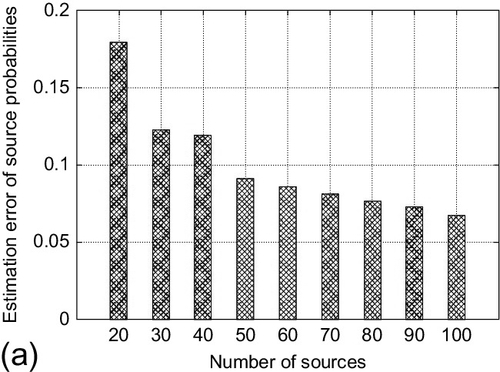
The first experiment showed the effect of the number of sources on prediction accuracy. The number of true and false claims was fixed at 1000 respectively. The average number of observations per source was set to 100. The number of sources is varied from 20 to 100. The estimation accuracy for both sources and claims is shown in Figure 4.1. We note that both estimation accuracy of source probabilities to be truthful and the claim classification accuracy (i.e., false positives and false negatives) improves as the number of sources increases. This is intuitive: more sources provide more corroborating observations about the claims, which helps the Bayesian approach to get better estimations. The usefulness of the Bayesian interpretation increases for large networks.

The next experiment shows the effect of changing the claim mix on estimation accuracy. The ratio of the number of true claims to the total number of claims in the network was varied. Assuming that there is usually only one variant of the truth, whereas rumors have more versions, one might expect the set of true claims to be smaller than the set of false ones. Hence, the total number of claims was fixed to be 2000 and change the ratio of true to total claims from 0.1 to 0.5. The c_true/c is set accordingly to the correct ratio used for the experiment. The number of sources in the network is set to 50 and the average observations per source is set to 100. The estimation accuracy for both sources and claims is shown in Figure 4.2. Observe that both the estimation error of source probabilities to be truthful and the error of claim classification increase as the ratio of true claims increases. This is because the true claim set becomes less densely claimed and more true and false claims are misclassified as each other as the number of true claims grows.

Finally, the Bayesian interpretation scheme was compared to three other fact-finder schemes: Sums (Hubs and Authorities) [35], Average-Log [37], and TruthFinder [36]. These algorithms were selected because, unlike other state-of-art fact-finders (e.g., 3-Estimates [38]), they do not require the knowledge about what mutual exclusion, if any, exists among the claims. In this experiment, the number of true and false claims is 1000 respectively, the number of observations per source is 150, and the number of sources is set to 50. The initial estimation offset on prior claim correctness was varied from 0.05 to 0.45. The initial claim beliefs of all fact-finders were set to the initial prior (i.e., 0.5) plus the offset used for the experiment. Each baseline fact-finder was ran for 20 iterations, and the 1000 highest-belief claims were selected as those predicted to be correct. The estimated probability of each source making a true claim was thus calculated as the proportion of predicted-correct claims asserted relative to the total number of claims asserted by source.

The compared results are shown in Figure 4.3. Observe that the prediction error of source correctness probability by the Bayesian interpretation scheme is significantly lower than all baseline fact-finder schemes. The reason is that Bayesian analysis estimates the source correctness probability more accurately based on Equation (4.34) derived in this chapter rather than using heuristic methods adopted by the baseline schemes that depends on the correct estimation on prior claim correctness. We also note that the prediction performance for claims in the Bayesian scheme is generally as good as the baselines. This is good since the other techniques excel at ranking, which (together with the hint on the number of correct claims) is sufficient to identify which ones these are. The results confirm the advantages of the Bayesian approach over previous ranking-based work at what the Bayesian analysis does best: estimation of probabilities of conclusions from observed evidence.

4.6 Discussion

This chapter presented a Bayesian interpretation of the most basic fact-finding algorithm. The question was to understand why the algorithm is successful at ranking, and to use that understanding to translate the ranking into actual probabilities. Several simplifying assumptions were made that offer opportunities for future extensions.

No dependencies were assumed among different sources or different claims. In reality, sources could be influenced by other sources. Claims could fall into mutual exclusion sets, such as when one is the negation of the other. Taking such relations into account can further improve quality of fact-finding. The change in posterior probabilities due to any single edge in the source-claim network was assumed to be very small. In other words, it is assumed that $|{\delta }_{i_{k}j}^t|\ll 1$ and $|{\eta }_{i{j}_k}^t|\ll 1$. It is interesting to extend the scheme to situations where a mix of reliable and unreliable sources is used. In this case, claims from reliable sources can help improve the determination of credibility of other sources.

The probability that any one source makes any one claim was assumed to be low. Hence, the lack of an edge between a source and a claim did not offer useful information. There may be cases, however, when the absence of a link between a source and a claim is important. For example, when a source is expected to bear on an issue, a source that “withholds the truth” exhibits absence of a link that needs to be accounted for.

In this chapter, we reviewed a novel analysis technique for information networks that uses a Bayesian interpretation of the network to assess the credibility of facts and sources. Prior literature that uses information network analysis for fact-finding aims at computing the credibility rank of different facts and sources. This work, in contrast, proposes an analytically founded technique to convert rank to a probability that a fact is true or that a source is truthful. This chapter therefore lays out a foundation for quality of information assurances in iterative fact-finding, a common branch of techniques used in data mining literature for analysis of information networks. The fact-finding techniques addressed in this chapter are particularly useful in environments where a large number of sources are used whose reliability is not a priori known (as opposed collecting information from a small number of well-characterized sources). Such situations are common when, for instance, crowd-sourcing is used to obtain information, or when information is to be gleaned from informal sources such as Twitter messages. The reviewed Bayesian approach shows that accurate information may indeed be obtained regarding facts and sources even when we do not know the credibility of each source in advance, and where individual sources may generally be unreliable.

Appendix

Consider an assertion C_j made be several sources $S_{i_1},\dots ,S_{i_K}$. Let $S_{i_k}{C}_j$ denote the fact that source $S_{i_k}$ made assertion C_j. It is further assumed that Equations (4.5) and 4.6 hold. In other words:

$\begin{array}{ll}\hfill \frac{P(S_{i_k}{C}_j|C_j^t)}{P(S_{i_k}{C}_j)}& =1+{\delta }_{i_{k}j}^t\hfill \\ \hfill \frac{P(S_{i_k}{C}_j|C_j^f)}{P(S_{i_k}{C}_j)}& =1+{\delta }_{i_{k}j}^f\hfill \end{array}$

where $|{\delta }_{i_{k}j}^t|\ll 1$ and $|{\delta }_{i_{k}j}^f|\ll 1$.

Under these assumptions, it can be proved that the joint probability $P(S_{i_1}{C}_j,S_{i_2}{C}_j,$$\dots ,S_{i_K}{C}_j)$, denoted for simplicity by P(Sources_j), is equal to the product of marginal probabilities $P(S_{i_1}{C}_j),\dots ,P(S_{i_K}{C}_j)$.

First, note that, by definition:

$\begin{array}{ll}\hfill P(Source{s}_j)& =P(S_{i_1}{C}_j,S_{i_2}{C}_j,\dots ,S_{i_K}{C}_j)\hfill \\ \hfill & =P(S_{i_1}{C}_j,S_{i_2}{C}_j,\dots ,S_{i_K}{C}_j|C_j^t)P(C_j^t)\hfill \\ \hfill & +P(S_{i_1}{C}_j,S_{i_2}{C}_j,\dots ,S_{i_K}{C}_j|C_j^f)P(C_j^f)\hfill \end{array}$

Using the conditional independence assumption, we get:

$\begin{array}{ll}\hfill P(Source{s}_j)& =P(C_j^t)\prod _{k=1}^{K}P(S_{i_k}{C}_j|C_j^t)\hfill \\ \hfill & +P(C_j^f)\prod _{k=1}^{K}P(S_{i_k}{C}_j|C_j^f)\hfill \end{array}$

Using Equations (4.5) and 4.6, the above can be rewritten as:

$\begin{array}{ll}\hfill P(Source{s}_j)& =P(C_j^t)\prod _{k=1}^{K_j}(1+{\delta }_{i_{k}j}^t)\prod _{k=1}^{K_j}P(S_{i_k}{C}_j)\hfill \\ \hfill & +P(C_j^f)\prod _{k=1}^{K_j}(1+{\delta }_{i_{k}j}^f)\prod _{k=1}^{K_j}P(S_{i_k}{C}_j)\hfill \end{array}$

and since $|{\delta }_{i_{k}j}^t|\ll 1$ and $|{\delta }_{i_{k}j}^f|\ll 1$, any higher-order terms involving them can be ignored. Hence, ${\prod }_{k=1}^{K_j}(1+{\delta }_{i_{k}j}^t)=1+{\sum }_{k=1}^{K_j}{\delta }_{i_{k}j}^t$, which results in:

$\begin{array}{ll}\hfill P(Source{s}_j)=& P(C_j^t)\left(1+\sum _{k=1}^{K_j}{\delta }_{i_{k}j}^t\right)\prod _{k=1}^{K}P(S_{i_k}{C}_j)\hfill \\ \hfill & +P(C_j^f)\left(1+\sum _{k=1}^{K_j}{\delta }_{i_{k}j}^f\right)\prod _{k=1}^{K}P(S_{i_k}{C}_j)\hfill \end{array}$

Distributing multiplication over addition in Equation (4.38), then using the fact that $P(C_j^t)+P(C_j^f)=1$ and rearranging, we get:

$\begin{array}{l}\hfill P(Source{s}_j)=\prod _{k=1}^{K_j}P(S_{i_k}{C}_j)(1+Term{s}_j)\end{array}$

where

$\begin{array}{l}\hfill Term{s}_j=P(C_j^t)\sum _{k=1}^{K_j}{\delta }_{i_{k}j}^t+P(C_j^f)\sum _{k=1}^{K_j}{\delta }_{i_{k}j}^f\end{array}$

Next, it remains to compute Terms_j.

Consider ${\delta }_{i_{k}j}^t$ as defined in Equation (4.5). The equation can be rewritten as follows:

$\begin{array}{l}\hfill {\delta }_{i_{k}j}^t=\frac{P(S_{i_k}{C}_j|C_j^t)-P(S_{i_k}{C}_j)}{P(S_{i_k}{C}_j)}\end{array}$

where by definition, $P(S_{i_k}{C}_j)=P(S_{i_k}{C}_j|C_j^t)P(C_j^t)+P(S_{i_k}{C}_j|C_j^f)P(C_j^f)$. Substituting in Equation (4.41), we get:

$\begin{array}{l}\hfill {\delta }_{i_{k}j}^t=\frac{P(S_{i_k}{C}_j|C_j^t)(1-P(C_j^t))-P(S_{i_k}{C}_j|C_j^f)P(C_j^f)}{P(S_{i_k}{C}_j|C_j^t)P(C_j^t)+P(S_{i_k}{C}_j|C_j^f)P(C_j^f)}\end{array}$

Using the fact that $1-P(C_j^t)=P(C_j^f)$ in the numerator, and rearranging, we get:

$\begin{array}{l}\hfill {\delta }_{i_{k}j}^t=\frac{(P(S_{i_k}{C}_j|C_j^t)-P(S_{i_k}{C}_j|C_j^f))P(C_j^f)}{P(S_{i_k}{C}_j|C_j^t)P(C_j^t)+P(S_{i_k}{C}_j|C_j^f)P(C_j^f)}\end{array}$

We can similarly show that:

$\begin{array}{ll}\hfill {\delta }_{i_{k}j}^f& =\frac{P(S_{i_k}{C}_j|C_j^f)-P(S_{i_k}{C}_j)}{P(S_{i_k}{C}_j)}\hfill \\ \hfill & =\frac{P(S_{i_k}{C}_j|C_j^f)(1-P(C_j^f))-P(S_{i_k}{C}_j|C_j^t)P(C_j^t)}{P(S_{i_k}{C}_j|C_j^t)P(C_j^t)+P(S_{i_k}{C}_j|C_j^f)P(C_j^f)}\hfill \\ \hfill & =\frac{(P(S_{i_k}{C}_j|C_j^f)-P(S_{i_k}{C}_j|C_j^t))P(C_j^t)}{P(S_{i_k}{C}_j|C_j^t)P(C_j^t)+P(S_{i_k}{C}_j|C_j^f)P(C_j^f)}\hfill \end{array}$

Dividing Equation (4.43) by Equation (4.44), we get:

$\begin{array}{l}\hfill \frac{{\delta }_{i_{k}j}^t}{{\delta }_{i_{k}j}^f}=-\frac{P(C_j^f)}{P(C_j^t)}\end{array}$

Substituting for ${\delta }_{i_{k}j}^t$ from Equation (4.45) into Equation (4.40), we get Terms_j = 0. Substituting with this result in Equation (4.39), we get:

$\begin{array}{l}\hfill P(Source{s}_j)=\prod _{k=1}^{K_j}P(S_{i_k}{C}_j)\end{array}$

The above result completes the proof. We have shown that the joint probability $P(S_{i_1}{C}_j,S_{i_2}{C}_j,\dots ,S_{i_K}{C}_j)$, denoted for simplicity by P(Sources_j), is well approximated by the product of marginal probabilities $P(S_{i_1}{C}_j),\dots ,P(S_{i_K}{C}_j)$. Note that, the proof did not assume independence of the marginals. Instead, it proved the result under the small ${\delta }_{i_{k}j}$ assumption.