Chapter 3
Information Synthesis in Multi-Granular Computing
Abstract
Humans usually learn things starting from local fragments, and gradually integrating them to form a global picture. On viewing an object from different abstraction levels, or different angles, they integrate the fragmentary and one-sided observations into systematic and overall understanding. This process is called information synthesis. Thus, information synthesis is the integration of information from different grain-size worlds. This is also one of the main issues in multi-granular computing. We present a mathematically synthetic model and use the model to deal with the synthesis of domains, topological structures, semi-order structures, and attribute functions respectively.
Keywords
attribute function; domain; information synthesis; semi-order structure; topological structureChapter Outline
3.2 The Mathematical Model of Information Synthesis
3.4 The Synthesis of Topologic Structures
3.5 The Synthesis of Semi-Order Structures
3.5.1 The Graphical Constructing Method of Quotient Semi-Order
3.5.2 The Synthesis of Semi-Order Structures
3.6 The Synthesis of Attribute Functions
3.1. Introduction
In Chapter 1, we presented a mathematical model, quotient space based model, for multi-granular computing. We show that a problem can be described by a triplet  . And we also discussed how corresponding quotient domain
  , quotient structure
  , and quotient attribute
  are constructed from original domain X, structure T and attribute f, respectively, i.e., a coarse grained space is constructed from a fine one.
In Chapter 2, we discussed one of the main characteristics of human problem solving, i.e., the multi-granular computing from coarse to fine, rough to detailed, and global to local hierarchically. Recall the example that we have mentioned, one always draws a draft of the whole building first, and then goes into its details, when designing a building. In our model, the analysis correspondingly goes from high to low abstraction levels through a hierarchical structure. The key issue of the computing is to establish the relationship between the quotient space and its original one.
However, the other scheme of multi-granular computing appears to be reverse, i.e., one usually learns things starting from local fragments, and gradually integrating them to form a global picture. On viewing an object from different abstraction levels, or different angles, integrate the fragmentary and one-sided observations into systematic and overall understanding. This process is called information synthesis, fusion, or combination.
Let us examine some examples.
Example 3.1
Gathering a series of information from topographic survey, geological prospecting, and seismic method, etc., in some region, then to predict mineral deposit of the region, is an information synthesis problem.
Example 3.2
Having front, top and side views of an object A, to determine its shape in three-dimensional space is an information synthesis problem. Here, each of the three views of the object is regarded as one of its quotient space representations. It is known that ‘projection’ is one of the typical approaches to quotient space representations. If object A is quite simple, its shape can be uniquely decided by its three views. Otherwise, we need some additional information, for example, some auxiliary views, cross-section views, or comments.
Example 3.3
A doctor takes a patient's temperature and pulse, examines the beat of the patient's heart using his stethoscope, and asks some questions. Then, the doctor makes a diagnosis and prescription. The process can be viewed as making a global decision from local observations. Each observation is a local understanding of the whole patient's physical condition in some abstraction level.
From the three examples, we can see that these problems can be transformed to that of constructing a synthetic problem representation from its quotient space representations. The key issue of information synthesis is to establish the relationship between the original space and its quotient space representations.
The aim of this chapter is to establish a mathematical model for information synthesis. The model is then applied to uncertain reasoning, planning, and other multi-granular computing problems.
3.2. The Mathematical Model of Information Synthesis
Given an unknown problem space , we have the knowledge of its two abstraction levels denoted by  and
and  , where
  and
and  are quotient spaces of X. A natural question to ask is how to have a new understanding of X from the known knowledge.
Example 3.4
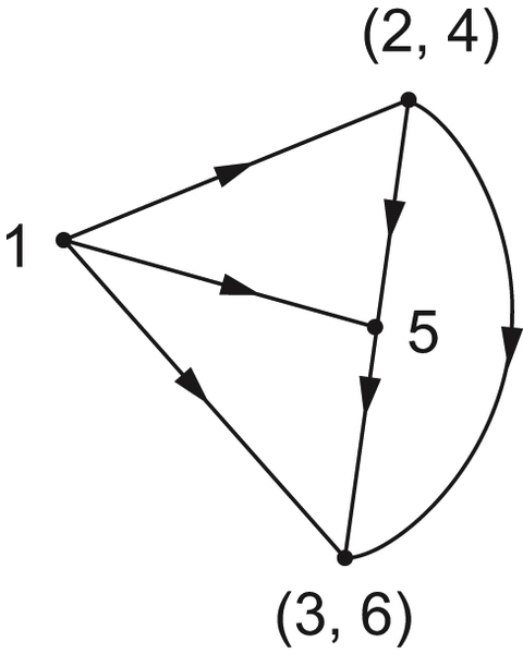
Assume that S is an object. Its front and top view are triangle  and
and  , respectively (see Fig. 3.1). How about its shape in three-dimensional space?
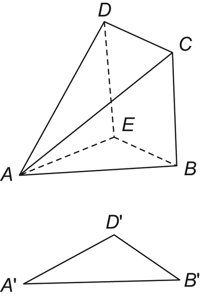
Only from its two projections (or two quotient spaces) in the example, we can't know its shape definitely, since there are infinite kinds of objects whose front and top views are identical with the two given triangles. If our domain is confined to be convex polyhedrons, S should be a kind of cone with A as its vertex, and its bottom consists of a convex polygon contained in quadrilateral BCDE, as shown in Fig. 3.1. If an additional constraint is given, for example, the volume of the object is maximal; the unique S can be identified.
Conversely, if less information is observed, for example, we only know that the front and top views of object S are arbitrary triangles, that is, the exact shape of the triangles is unknown, the constraints on the shape of S will be more relaxed.
In a word, if we are given the knowledge about A in some abstraction levels, generally, we can only have a new understanding about A at the level that is just one (finer) level below them. The complete details of A may not necessarily be known.
We may have the synthetic rules as follows.
Assume that and are the knowledge about  in two different abstraction levels. The synthesis of and is defined as a new abstraction level of A, denoted by
  , which satisfies the following three basic synthetic principles.
(1) and are quotient spaces of 
(2)  and
and  are quotient structures of
  corresponding to
(3)  and
and  are projections of f on and , respectively.
Space also needs to satisfy some optimal criteria generally.
We next discuss the synthesis of domain, structure and attribute function, respectively.
3.3. The Synthesis of Domains
Assume that and are quotient spaces of . and correspond to equivalence relations  and
and  , respectively.
Define the synthetic space of and as follows, where  is an equivalence relation corresponding to
![]()
Example 3.5
X is the staff members of an organization.
Based on education received, the X is classified as follows, and is called a-classification.
X can also be classified in terms of age, and is called b-classification.
The synthesis of these two classifications is that x and y belong to the same synthetic class  x and y belong to both the same a-class and the same b-class.
If there is no additional information, from these two partitions, we can only have education-level-based and age-based partitions. No more information such as sex can be known.
It is known that all equivalence classes on X form a semi-order lattice, under the set inclusion relation  if
if  .
.
In terms of the semi-order lattice, the synthesis of and can be defined as follows.
Definition 3.1
Assume that and are two equivalence relations on X. If is the least upper bound of and in the semi-order lattice, then is the synthesis of and . Meanwhile, the synthesis can also be defined by partition. If  and
and  are two partitions with respect to and , respectively, then the synthesis of and can be represented by
![]()
We next show that the two definitions above are equivalent.
Proof
If  , then
  and
and  .
.
Where, symbol ‘∼’ denotes an equivalence relation on .
From Example 3.5, we have the synthesis of both educational-level- and age-based partitions as follows.
Obviously, space  defined above satisfies the synthetic principles. That is, both and are quotient spaces of . is the finest space, which we can get from quotient spaces and . It is also the coarsest one among the spaces which satisfy the synthetic principles. That is, it is the least upper bound. Since in some sense it is optimal, it is reasonable to regard as a synthetic space of and .
3.4. The Synthesis of Topologic Structures
We now discuss the synthesis of structures. As mentioned before, there are three kinds of common structures. That is, topologic, semi-order, and operation-based structures. In this section, we only discuss the synthesis of topologic structures.
Assume that and are quotient spaces of . Structure , the synthesis of and , is defined as follows.
Definition 3.2
The synthetic structure of and is the least upper bound of and , in the semi-order lattice that consists of all topologic structures on X.
Obviously, satisfies the synthetic principles. That is, and are the quotient topologies of on quotient spaces and , respectively. is the coarsest one, among the topologies whose quotient topologies are and .
Let  . is the topology with B as its base, i.e., consists of all possible sets obtained from any union operations on the elements of B.
Example 3.6
3.5. The Synthesis of Semi-Order Structures
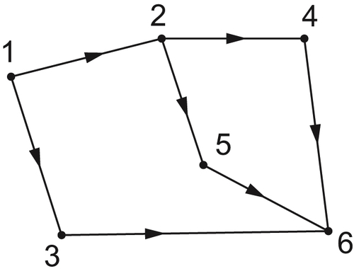
Semi-order is a common structure. Especially when X is a finite domain, many structures can be represented by a directed acyclic graph that can be described by a semi-order. So semi-order is one of the most popular structures.
3.5.1. The Graphical Constructing Method of Quotient Semi-Order
In Chapter 1, we have introduced a method for constructing quotient semi-order. The constructing process follows the line: semi-order  right-order topology quotient topology quotient quasi semi-order. Finally, the quotient semi-order on quotient space [X] is defined by the quotient quasi semi-order. It has been proved that the approach is complete. That is, if there is a quotient semi-order in [X] such that its natural projection p is order-preserving, then the quotient semi-order can be obtained by the approach. And in the ‘minimum’ sense, the quotient semi-order obtained is unique and optimal. But the approach, after all, is not straightforward, since the quotient semi-order must be defined by means of topology.
We next present a direct method for constructing quotient semi-order, when [X] is finite.
Definition 3.3
(1)  ,
,
(2)  , there exists a sequence
  of finite elements in D such that
  .
.
Then, D is called a semi-order base of T.
The condition (2) above can be restated as , there exists a sequence  of finite points such that
  and
and  .
.
Example 3.7
Proposition 3.1
Definition 3.4
![]()
Obviously, if there is no directed loop on the directed network corresponding to the quasi semi-order on [X], then, in fact, the quasi semi-order is a semi-order. Thus, there exists a quotient semi-order on [X]. From the definition of quotient semi-order, it is easy to know that the quotient semi-order has order-preserving and is minimal.
Proposition 3.2
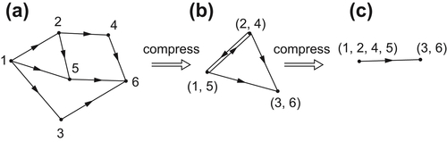
From Definition 3.4, we know that constructing a directed network  (it might have directed loops) from a directed network
  is identical with the ‘compression’ operation of directed graph on graph theory.
If there are directed loops on , compressing the nodes on each directed loop into one node, then we have a directed network without loops that just corresponds to the semi-order space with respect to R obtained by the mergence method in Section 1.4.
Example 3.8
Compressing into  , as shown in Fig. 3.3(b), then we have a directed loop. Merging the directed loop into one node, we have a semi-order space
  , as shown in Fig. 3.3(c). The semi-order corresponding to is just the quotient semi-order obtained by the mergence method.
Now, we find the least upper bound of quotient semi-order of space with respect to R, by using the decomposition method presented in Section 1.4.
Decomposing  , we have
  .
.
Decomposing  , we have
  .
.
Similarly,  .
.
When [X] is finite, it’s known that a quotient semi-order can directly be constructed by using directed networks. Moreover, when [X] is an infinitely countable set, the direct approach is still available.
3.5.2. The Synthesis of Semi-Order Structures
Assume that and are two quotient spaces of X. If there exist semi-orders on and , then we have two semi-order spaces and . Now, we find their synthetic semi-order space  that satisfies the synthetic principle, i.e., is the least upper bound of and , and are quotient semi-orders of on and , respectively.
Now, the following two questions must be answered. In what condition does the synthetic semi-order space exist? If it exists, then how to construct such a space .
1. The synthetic procedure of semi-order spaces-topology based method
Semi-order spaces and are given. The synthetic procedure is as follows.
(1) Find the least upper bound of and denoted by .
(2) Find the right-order topologies corresponding to and , denoted by  and
and  , respectively.
(3) Find the synthetic topology  of and on . And topology is the least upper bound of and on .
(4) Find the semi-order from , and denoted by .
Finally, is the synthetic semi-order space.
Example 3.9
find the synthetic semi-order space .
(1) Find , , where
(2) Find the right-order topologies and of and , respectively. Their corresponding topologic bases are
(3) Find the synthetic topology . Its corresponding topologic base is
Obviously, the quotient semi-order structures of on and are just and , respectively.
Theorem 3.1
(1) is a semi-order on
(2) Mapping  is order-preserving
(3) is the coarsest one among semi-order structures which satisfy the conditions (1) and (2).
Proof
Since is the least upper bound of and . For  there exist
  and
and  such that
  .
.
Let  be a minimum open set on
  containing
  .
.
Obviously,  is a minimum open set on containing x, since topology is the least upper bound of and .
Assume that  ,
,  . We next show that
  .
.
Let  and
and  , where
  and
and  . From
  , we have
  .
.
Thus,  and
and  is an open set containing
  . Then,
  .
.
Similarly, 
Since is a semi-order on , we have  .
.
Similarly,  , i.e., is a semi-order on .
Next, we show that is order-preserving.
Assuming  , we have
  .
.
By letting , we have  , i.e.,
  .
.
Carrying out operation  on
on  , we have
  since
since  is a set on .
From  ,
,
That is, is order-preserving.
Similarly,  is order-preserving.
Finally, we show that is the coarsest one.
Assume that  satisfies the conditions (1) and (2) of Theorem 3.1 and is coarser than .
Let  and be the corresponding right-order topologies of
  and , respectively. Since is coarser than , we know that is coarser than . And both and are quotient topologies of . This contradicts that is the coarsest one among topologies whose quotient topologies are and , or is the least upper bound of and .
Therefore, is the coarsest one among semi-order structures which satisfy the conditions (1) and (2).
From Theorem 3.1, it’s known that is the coarsest one among semi-order structures which satisfy the conditions (1) and (2). This means that provides the maximum information regarding the relation among the elements on , when the only known knowledge is and . Therefore, is the ‘optimal’ synthetic structure.
2. The direct method for synthesizing semi-order spaces
In the above topology-based method, we first synthesize the right-order topologies corresponding to the given two semi-order structures and , then find the synthetic semi-order. This is not a straightforward method. We now provide a new approach that constructs the synthetic semi-order from semi-order structures and directly.
Directed Method
(1) Find the least upper bound of spaces and .
(2) For  let and , where and .
Define  and
and  . Especially, if , then . The relation defined above is denoted by
  .
.
We now show that is just the same semi-order on as that obtained by the above topologic method.
Proposition 3.3
Proof
![]()
![]()
![]()
![]()
![]()
We have  .
.
Example 3.10
Find the synthetic space by the direct method.
Solution
![]()
![]()
![]()
Find from the direct method.
Since  and
and  , we have
  .
.
Again  and
and  , we have
  .
.
…
Since and  are incomparable and
  , then
  and
and  are incomparable as well.
Finally, we have as the same as is shown in Fig.3.5.
Theoretically, since a semi-order structure can be transformed into a topologic structure, the former can be regarded as a special case of topologic structures. For example, the order-preserving property between a semi-order space and its quotient space, in essence, mirrors the continuity of projecting a topologic space on its quotient space. In addition, the ‘coarsest’ property of the synthetic semi-order represents the ‘coarsest’ property of the synthetic topology.
Although there is no difference between semi-order and topologic structures in theory, the former has widespread applications in reality. Especially, when domain X is a finite set, a semi-order can be represented by a directed network. Based on the network representation, a quotient semi-order can be obtained from its original semi-order directly. And a synthetic semi-order can also be obtained from semi-order structures directly; there is no need to transform it into topologic structures. This will make things convenient for the applications.
3.6. The Synthesis of Attribute Functions
For a problem space , given the knowledge of its two abstraction levels and , we intend to have an overall understanding about .
Assume that the overall understanding of is represented by . We are now going to discuss how to construct  from and such that it satisfies the synthetic principles.
3.6.1. The Synthetic Principle of Attribute Functions
Given a problem space and its quotient spaces and . Let  , be nature projections.
  is an equivalence relation with respect to quotient space
  .
.
Fixing projection ,  is uniquely defined. When T is a topology, including a semi-order, fixing ,
  is also uniquely defined.
Once the approach of constructing the global attributes of set A from its local information is determined, projection  is uniquely defined too.
Conversely, two spaces and are given. Let . Their synthetic space must satisfy the following three conditions at least
 (3.1)
(3.1)
In general, the solution satisfying constraints (3.1) is not unique. In order to have a unique solution, additional optimization criteria have to be provided generally. In Section 3.3, the optimization goal of the synthetic space is represented by ‘the least upper bound’ criterion. In Section 3.4, the optimization goal of the synthetic topology is indicated by ‘the coarsest’ criterion.
We now present the synthetic principle of attribute functions as follows.
Given and , find the synthetic space satisfying the following conditions.
(1) 
 , is a natural projection.
![]() (3.2)
(3.2)
(2) Assume that  is a given optimization criterion. Then which satisfy Formula (3.2).
![]() (3.3)
(3.3)
We next show the rationality of the above synthetic principles.
The condition (1), i.e.,  , is necessary. That is, the projections of on and must be identical with the given and , respectively. As shown in Example 3.4, the corresponding projections of the object S synthesized from the given front and top views have to be identical to the given triangles and at least, respectively, as shown in Fig. 3.1.
In fact, the solution satisfying constraint (3.2) is not unique. This is not necessarily a bad thing. For example, when designing a mechanical part, we have to consider several requirements and each requirement can be regarded as a kind of constraint on its abstraction level. Generally, the design result satisfying these requirements is not unique. This means there is plenty of room for designers’ imaginations. The design works will benefit from the variety of the results. But this is an obstacle to a computer while it is not intelligent enough. So in computer problem solving, some sort of optimization criteria are needed.
Condition (2) above is one such optimization criterion. As long as it is given, the computer will be able to find the optimal solution. For example, we design a container in order to satisfy the requirements shown in Fig. 3.1. That is, its front and top views are triangles and , respectively. For human designers, under such requirements, an infinite variety of designs can be envisioned. But, in order to have a solution by a computer, a specific criterion must be provided. For example, if taking the maximal volume of the container as a criterion then a cone ABCDE shown in Fig. 3.1 will be turned out.
Generally, the optimal synthetic criteria are domain-dependent and hard for computers to implement. In reality, we can only have some so-called satisfactory solutions. This is one of the main ideas in artificial intelligence.
In fact, in the real world, the situation is more complicated. For example, the information that we have in some abstraction level is not precise. Therefore, we have to handle the imprecise or incomplete information.
We are given spaces and . Let be a synthetic space.
Let  be a space consisting of all attribute functions on . Assume that there exists a metric
  in each such that
  ,
,  , , is a metric space.
Now, if the observation in level  is not precise, so Formula (3.2) may not hold accurately. Similar to the method of least-squares, we establish the following relation.
 , is a natural projection. And
 .
.
![]() (3.4)
(3.4)
![]() (3.5)
(3.5)
If function satisfying Formula (3.5) is still not unique, an additional criterion is needed, for example, an additional function  . By letting as well.
![]() (3.6)
(3.6)
Attribute function that obtained from and by Formulas (3.4) and (3.5), or by Formula (3.6), is a synthetic one.
As mentioned above, the optimization synthetic criteria are generally domain-dependent, and there is a great variety of methods for extracting global information from local ones, i.e., a variety of functions. Therefore, it is hard to have a universal optimization criterion.
3.6.2. Examples
In this section, we will explain the computed tomography, CT for short, by our synthetic model in order to have a better understanding of the model.
Example 3.11
As shown in Fig. 3.6, T is a biological tissue under study, by placing an X-ray and photosensitive film DE alongside the tissue so that it lies perpendicular to the incident rays. When the X-ray traverses from left to right along the x-axis, an image on film DE of X-ray attenuation during this traverse is obtained. The image of the tissue's structure can be reconstructed by using a computer to analyze a set of these recorded images. This is the basic principle of computed tomography (Kak and Slaney, 2001).
When a beam of X-rays penetrates any structure shown in Fig. 3.6, attenuation occurs, the degree of the attenuation is related to: (a) the atomic number of the element of which the structure is composed, or the effective atomic number of a complex structure and (b) the concentration of the substances forming that structure. Thus, the density of electrons, or effective electron density, determines the degree to which a given beam of X-rays will be attenuated. Therefore, from the attenuation of the X-ray the structure of a tissue being tested can be known.
In Fig. 3.6, we now assume that  is the attenuation coefficient of that tissue at (x,y) in one of its cross-sections. When X-ray passes through the given structure, the density of the beam emerging from the other side of the structure will depend on
  . The one-dimensional image recorded in film DE is
![]() (3.7)
(3.7)
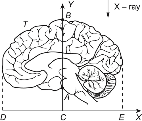
In terms of hierarchical model, the attenuation coefficient  can be regarded as an attribute function of a problem space , where is a part of two-dimensional Euclidean space, e.g., a cross-section of a tissue as shown in Fig. 3.6.
From Formula (3.7), we can see that  is a projection of on X. It forms a new space , where is a quotient space of by considering each line perpendicular to the x-axis as a point, i.e., an equivalence class. Thus, is a line segment DE on the x-axis. The relation between attribute functions and g(x) is the following.
![]()
For each line  intersecting the x-axis with angle
  , we have a projection
  .
.
For all  , we have a set
  of projections. Then, we obtain a set of quotient spaces denoted by
  , .
, .
The point is how to find from a set , of quotient spaces. This is the same problem that CT intends to solve.
From the hierarchical model viewpoint, it is to find a synthetic space from a given set of quotient spaces. That is, given  , we find a
  such that it satisfies:
 : X →
: X →  is a projection, is a domain of
  (s).
(s).
![]() (3.8)
(3.8)
Letting  , we have
In mathematics, it can be proved that a set of equations (3.8) has a unique solution. So there is no need of additional criteria in the synthetic model. The synthetic attribute function can be obtained by solving Formula (3.8) directly.
From the theorems of Fourier transform, we have the following theorem.
Theorem 3.2
The Fourier transform of the one-dimensional projection of a two-dimensional function is identical with the distribution on the central section of the Fourier transform of that function.
The theorem can be stated by the following mathematical formulas.
The Fourier transform of function is as follows.
The projection of on X is
The Fourier transform of  is
is
Let  , we have
  .
.
By Fourier inverse transform of  , we have
Therefore, from a given set , we have a Fourier transform . Meanwhile, from the Fourier inverse transform of , we finally have . In CT, corresponds to the image of the biological tissue being radiographed. Thus, the computed tomography is a special case of our synthetic problem, while there is no need for the optimal criteria.
Example 3.12
In reality, the reconstruction of by the method indicated in Example 3.11 may not be feasible, since an infinite number of projections are needed. For this reason, Kashyap and Mittal (1975) presented a minimization approach to algebraic equations. We first briefly explain their approach in the way of our hierarchical model.
(1) Discretization
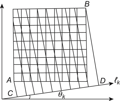
Assume that the domain X of is a square. Then, each edge of the square is equally divided into n intervals. We have a mesh consisting of n×n blocks. Regarding each block as a point, the value of at its center is considered as the value of in that block.
Regarding each block as an equivalence class, the mesh is a quotient space denoted by X. Taking the value of at the central point of each block as the value of in the block, which is called the inclusion principle, one of the basic approaches for constructing global information as mentioned in Chapter 2.
(2) Projection
![]()
Then,  is a problem space after the discretization.
We draw a radial lk that intersects the horizontal line at angle  . From vertexes A and B, we draw two lines perpendicular to lk at points C and D, respectively. Then, line CD is divided into n intervals equally. From each end point of the intervals we draw a line perpendicular to lk and have n regions of square X (Fig. 3.7). From left to right, the regions are denoted by
  , respectively.
Let  .
.
Obviously,  is a quotient space of X.
Define  .
.
That is,  is the sum of
  over the range of region
  , or denoted by
  for short.
Define  .
.
Therefore,  is a quotient space of .
Given t projections  , we find their synthetic space . This is just the problem that CT intends to solve.
(3) Minimization
Changing the subscript of the vector f, we have  . Let
. Let  be a
be a  matrix. Then
![]()
From the synthetic principles, f must satisfy the following formula. .
.
![]() (3.9)
(3.9)
From linear algebra, we know that if  , then Equation (3.9) has a unique solution. The f obtained from Equation (3.9) is the synthetic attribute function, or the image of biological tissue being examined after discretization.
If t>n generally, there is no solution to Equation (3.9). Similar to the method of least-squares, we construct a metric function  in t × n dimensional Euclidean space. Let
![]() (3.10)
(3.10)
The synthetic attribute function f is the one that makes the right hand side of Formula (3.10) minimum.
If t<n, Equation (3.9) has an infinite solution. It is necessary to introduce an optimal criterion such as
![]() (3.11)
(3.11)
From Lagrange multiplier procedure, we have
![]() (3.12)
(3.12)
Finding the minimum of Formula (3.12), we have
![]() (3.13)
(3.13)
Since (I+C) is not singularity, we have
![]()
That is,
![]()
Since when t<n, B is not singularity, using pseudo-inverse we have is the transpose of matrix B.
![]()
Finally, we have  , where
  . f is the synthetic attribute function, i.e., the function corresponding to the sectional images after discretization in computed tomography.
Next, we give a mathematical example which can be regarded as an application of the synthetic model.
Example 3.13
X is a linear normed space. Given a  , since itself may be rather complicated, we project f on a simpler space, for example, a real number axis. Assume A
 X∗, where X∗ is a conjugate space of X, i.e., X is a space consisting of all linear bounded functionals on X. For
  , functional
  is known. The problem is how to deduce f from g(f). By the synthetic viewpoint, it means that constructing f from the known ,.
Let L(A) be a linear sub-space on X∗ containing A. Fixed f, varying within L(A), then is a linear functional on L(A), and is denoted by  . Assuming
  ,
, .
.
Assume further that  is a canonical mapping which embeds X within X∗∗ and there exists c−1. By letting
  ,
,  is just the synthesis of ,.
Assume that X is a Euclidean space.
A set of equations is given below.
 (3.14)
Regarding vector  as a point in space En and
  as a value of linear functional
  at point x. Letting
  , L(A) is a sub-space supported by m vectors.
If  , Formula (3.14) has a unique solution, i.e.,
  . If
. If  is a proper subset of
  , Formula (3.14) has an infinite number of solutions. Then, we introduce an optimal criterion
![]()
The example shows that solving a set of equations, or a constraint satisfaction problem, can be regarded as information synthesis.
In Chapter 4, uncertain reasoning will be studied by the synthetic model.
3.6.3. Conclusions
In this section, we present a synthetic model under the quotient space theory.
Spaces and are given. is their synthetic space. We have
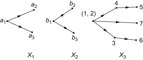
(1) The synthesis of domains: X3 is the least upper space of X1 and X2
(2) The synthesis of topological structures: T3 is the least upper topology of T1 and T2.
(3) The synthesis of attribute functions: f3 satisfies the following condition , where  , is a natural projection. If and have error, then the above formula will be replaced by the following formula.
![]()
Where  is a metric function on , is all attribute functions on , and the min operation is carried out on all attribute functions f on X3.
If the solution is not unique, a proper optimal criterion must be added in order to have an optimal solution.
The synthetic model can be applied to constraint satisfaction problems, reasoning processes, etc.
..................Content has been hidden....................
You can't read the all page of ebook, please click here login for view all page.