![]()
6.4. The Comparison between Statistical Heuristic Search and  Algorithm
6.4.1. Comparison to 
Are the constraints given in Hypothesis I, including relaxed cases, strict? In order to unravel the problem, we'll compare them with well-known  search.
Definition 6.8
Assume that  is an admissible estimate of
  , i.e.
  . If for
  , we have
  , where
  is the distance between
  and
and  , then
  is called reasonable, i.e., monotonic and admissible.
Proposition 6.2
Assume that G is a uniform m-ary tree and  is estimate with a typical error of order
  [Pea84].
  is reasonable.
  is i.i.d. and has a finite fourth moment. If A∗ algorithm using
  as its evaluation function has the polynomial mean complexity, then SA search using
  as its statistic also has the polynomial mean complexity.
Proof
Assume that  ,
,  and
and  . Since
  is reasonable, we have
  .
.
Since  is an admissible estimate having a typical error of order
  and
and  searches g with polynomial complexity, from Property 6.1 in Section 6.1.1, we have that
  , there exists
  (ε is independent of p) such that
It does not lose generality in assuming that  . We now estimate the difference between
  and
and  .
.
For the part satisfying  , we have:
![]()
![]()
![]()
Thus, we have:
![]()
![]()
Let  , where
  . We have:
![]() (6.19)
(6.19)
Letting  be the local statistic of nodes, we have that when
  ,
,  holds. From Formula (6.19), when
  , for subtree
  if using the ‘mean’ of local statistics as its global statistic, then the global statistic from
  ,
,  , is
, is  , and the global statistic from
  ,
,  , is
, is  , i.e., the latter is larger than the former. Moreover,
  is equivalent to
  that belongs to the mixed cases we have discussed in Section 6.3.2. The mean complexity of the corresponding SA is polynomial.
The proposition shows that if  is monotonic, when
  is convergent SA is also convergent.
From Theorem 6.6, it’s known that the proposition still holds when  is not monotonic.
Proposition 6.3
Assume that  is the lower estimation of
  with a typical error of order
  . Let
. Let
![]()
If  has a finite fourth moment,
  and
and  ,
,  , where d is a constant, letting
  be a local statistic of nodes, then SA search is convergent.
Proof
Assume that  and
and  . We have
![]()
![]()
![]()
![]()
![]()
![]() (6.20)
(6.20)
Let  . When
  , we have:
![]()
From Theorem 6.6, the corresponding SA is convergent.
The proposition shows that all lower estimations  of
of  that make
  search convergent, when using the
  as a local statistic, we can always extract a properly global statistic from
  such that the corresponding SA search is convergent.
We will show below that the inverse is not true, i.e., we can provide a large class of estimations  such that its corresponding SA is convergent but the corresponding
  is divergent.
Proposition 6.4
Assume that  is a lower estimation of
  and is an
  random variable with a finite fourth moment. For
  ,
,  , where c is a constant and
  . If
. If  is the local statistic of node n, then the corresponding SA is convergent.
Proof
From  ,
,  , we have
  . Letting
  and
and  , we have
![]()
![]()
From Theorem 6.6, the corresponding SA is convergent.
Corollary 6.6
Assume that  is a lower estimate of
  with a typical error of order N and
  has a finite fourth moment. For
  ,
,  , where c is a constant and
  . Letting
  be a local statistic of nodes n, the corresponding SA is convergent.
Proof
Since  is a lower estimate with a typical error of order N from its definition, there exists
  such that
  ,
,  .
.
We have: . From Proposition 6.3, we have the corollary.
![]()
According to Pearl’s result, under the conditions of  in Corollary 6.6 the corresponding
  is exponential, but from Corollary 6.6 SA is convergent. Therefore, the condition that SA search is convergent is weaker than that of
  search.
Corollary 6.7
If  is a lower estimate,
  has a finite four moment, for
  ,
,  are equal, and there exist
  and
and  such that
  , then Corollary 6.6 holds.
Corollary 6.8
If  is the lower estimate of
  with a typical error of order
  ,
,  has a finite fourth moment and
  ,
,  , where d is a constant, then the corresponding
  is convergent. Letting
  be the local statistic of node n, the corresponding SA is also convergent.
Proof
From Proposition 6.2 and the Pearl’s result given in Property 6.4, the corollary is obtained.
From the above propositions, it’s easy to see that the condition that makes SA convergent is weaker than that of  . On the other hand, the convergence of
  is related to estimation with a typical error of order
  that is defined by Formulas (6.1) and (6.2). It’s very difficult to confirm the two constants
  and
and  within the two formulas. So the convergent condition of
  is difficulty to be tested. But in SA, the only convergent requirement is that statistics
  are independent and have positive variances and finite fourth moments. In general, the distribution of
  satisfies the conditions.
6.4.2. Comparison to Other Weighted Techniques
The statistical inference methods can also be applied to weighted heuristic search. Weighted techniques in heuristic search have been investigated by several researchers (Nilson, 1980; Field et al., 1984). They introduced the concept of weighted components into evaluation function  . Thus, the relative weights of g(n) and h(n) in the evaluation function can be controlled by:
 is a weight.
![]()
![]()
![]()
In statically weighted systems, a fixed weight is added to the evaluation functions of all nodes. For example, Pearl investigates a statically weighted system  and showed that the optimal weight is
  (the definition of
  and more details see Pearl (1984b)). But even the optimal weight is adopted; the exponential complexity still cannot be overcome.
For dynamic weighting, for example, the weight  may vary with the depth of a node in the search tree, for example,
  , where e is a constant and N is the depth that the goal is located. But the dynamic weighting fails to differentiate the nodes: which are on the solution path (
 ), whereas the others (
 ) are not. Thus, neither static nor dynamic weighting can improve the search efficiency significantly.
As stated in Section 6.1.1, under certain conditions we regard heuristic search as a random sampling process. By using the statistic inference method, it can tell for sure whether a path looks more promising than others. This information can be used for guiding the weighting.
For example, the Wald sequential probability ratio test (SPRT) is used as a testing hypothesis in SA search. In some search stage if the hypothesis that some subtree T in the search tree contains solution path is rejected, or simply, subtree T is rejected, then the probability that the subtree contains the goal is low. Rather than pruning T as in SA, a fixed weight  is added to the evaluation function of the nodes in T, i.e. the evaluation function is increased by
  ,
,  . If the hypothesis that the subtree T′ contains the goal is accepted, the same weight is added to evaluation functions of all nodes in the brother-subtrees of T′, whose roots are the brothers of the root of T′. If no decision can be made by the statistic inference method, the searching process continues as in SA search. We call this new algorithm as the weighted SA search, or WSA. It is likely that the search will focus on the most promising path due to the weighting. We will show that the search efficiency can be improved by the WSA significantly.
For clarity and brevity, we assume that the search space is a uniform 2-ary tree,  , in the following discussion. The SPRT (or ASM) is used as a testing hypothesis and the given significance level is
  , where
  . The complexity of an algorithm is defined as the expected number of the nodes expanded by the algorithm when a goal is found.
ƒ(n) is an arbitrary global statistic (a subtree evaluation function) constructed from heuristic information and satisfies Hypothesis I.
1. Weighting Methods
There are two cases.
Formula  means there exist constants D and E such that
 .
.
![]()
In the weighted SA, the weighting method is
![]() (6.21)
(6.21)
![]()
The weighting method is
![]() (6.22)
(6.22)
2. Optimal Weights and the Mean Complexity
The weighted function is  ,
,  is a constant.
Definition 6.9
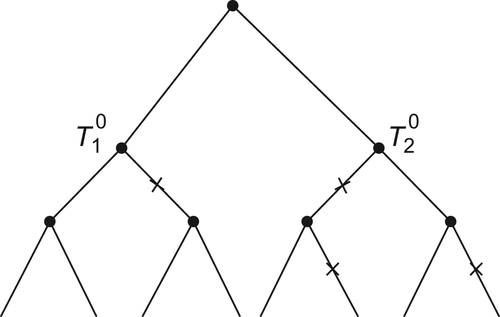
A subtree is called a completely weighted, if all its subtrees have been judged to be rejected or accepted.
The subtree  shown in Fig. 6.8 is completely weighted (where the rejected subtrees are marked with sign ‘
 ’ ). But subtree
  is not completely weighted.
We imagine that if a subtree is not completely weighted, the testing hypothesis is continued until it becomes a completely weighted one. Obviously, a completely weighted subtree has more expanded nodes than the incompletely weighted one. Thus, if an upper estimate of the mean complexity of the completely weighted subtree is obtained, it certainly is an upper estimate of the mean complexity in general.
We now discuss this upper estimate.
Let T be a completely weighted 2-ary tree and  be a set of nodes at depth d. For
  , from initial node
  to n there exists a unique path consisting of d arcs. Among these d arcs if there are i
  arcs marked by ‘
 ’, node n is referred to as an i-type node, or i-node.
So  can be divided into the following subsets:
In considering the complexity for finding a goal, we first ignore the cost of the statistic inference. Assume that the goal of the search tree belongs to 0-node so that its evaluation is  , where N is the depth at which the goal is located. From algorithm
  , it's known that every node which
  must be expanded in the searching process.
If node n is an i-node, its evaluation function is  . All nodes whose evaluations satisfy the following inequality will be expanded.
![]()
From  , it’s known that the complexity corresponding to the evaluation function
  is
is  . The mean complexity of each i-node (the probability that an i-node is expanded) is
![]()
On the other hand, the mean complexity for finding a goal at depth N is at least N. Thus the mean complexity of each i-node is
![]()
![]()
When the goal is a 0-node, the upper bound of the mean complexity for computing all d-th depth nodes is the following (ignoring the complexity for making statistic inference).
![]()
![]()
![]()
On the other hand, when  is a constant, from Section 6.2 it’s known that the mean computational cost of SPRT is a constant Q for making the statistic inference of a node. When the goal is an 0-node, accounting for this cost, the mean complexity for computing all d-th depth nodes is
![]()
Similarly, if the goal belongs to i-node, its evaluation is  . Then the computational complexity of each node in the search tree is increased by a factor of
  . Thus when the goal is an i-node, the mean complexity for computing all d-th nodes is
![]()
From algorithm SA, the probability that the goal falls into an i-node is  if the given level is
  ,
,  . At depth N, there are
  i-nodes, so the probability that the goal belongs to i-node is
![]()
Accounting for all possible cases of the goal node, the mean complexity for computing all d-th depth nodes is
![]()
![]()
Let  . There is an optimal weight
  such that
  is minimal. The optimal weight
  and
and  .
.
The upper bound of mean complexity of WSA is
![]()
Letting  , we have
 is a constant.
 (6.23)
Theorem 6.10
Assume  ,
,  . There exists an optimal weight
  such that
![]()
The complexity of WSA by using the optimal weight is
![]()
Proof
Let  , i.e.,
  . From
  , we have
![]()
We obtain
![]()
Let  .
.
If  , for any
  , we have
![]() (6.24)
(6.24)
Substitute (6.24) into (6.22), we have
![]()
Thus,  .
.
From the theorem, we can see that the whole number of nodes in a 2-ary tree with N depth is  ,
,  . Therefore, when
  as long as
  then we have
  .
.
Theorem 6.11
If  , letting
  and using the weighted function
  , then
  .
.
Proof
Similar to Theorem 6.10, we have
![]()
Let  . There exists an optimum
  such that
  is minimal. Substituting
  into the above formula, we have
![]()
Letting  , we have
  .
.
Thus, when 
 .
.
Finally,  .
.
3. Discussion
The estimation of c and a: Generally, whether  is either
  or
or  is unknown generally. Even if the type of functions is known but parameters c and a are still unknown.
We propose the following method for estimating c and a
Assume that in the 2k level, the number of expanded nodes is  . Then
  can be used to estimate c. If c does not change much with k, then
  may be regarded as type
  , where
  .
.
If c approaches to zero when k increases, then we consider  . If
. If  is essentially unchanged, then
  is regarded as type
  and
and  .
.
Alterable significance levels: Assume that  is the optimal weight for
  . Value
  is unknown generally. We first by letting
  then have
  . Letting
  , we have
![]()
![]()
In order to have  , b should be sufficiently small such that
 (6.25)
Since c is unknown, b still cannot be determined by Formula (6.25). In order to overcome the difficulty, we perform the statistical inference as follows. For testing i-subtrees, the significance level we used is  , where
  is a series monotonically approaching to zero with i. Thus, when
  is sufficiently small, Formula (6.25) will hold. For example, let
  , where b is a constant and
  is a significance level for testing i-subtrees.
From Section 6.2, it’s known that when using significance level  the mean complexity of the statistical inference is
![]()
Thus, replacing Q by  in Formula
  , when significance level is
  we have
![]()
Theorem 6.12
If  ,
,  is a constant, letting the significance level for i-subtrees be
  , where b is a constant, then
![]()
Alterable weighting: When the type of the order of  is unknown, we uniformly adopt weight function
  . Next, we will show that when
  ,
,  , if the weight function
  is used what will happen to the complexity of WSA.
Since  the ‘additive’ weight s can be regarded as ‘multiplicative’ weight
  but
but  is no long a constant. So we call it the alterable weighting.
Assume that  . When a node is a 0-node,
  . For any node
  , it is assumed to be an i-node. The evaluation function of
  after weighting is
  , where
  are the weights along the path from starting node
  to node
  .
.
According to the heuristic search rules, when  , i.e.,
  , node
  will be expanded.
It’s known that the goal locates at the N level, so the evaluation  may be adopted.
Thus, when s fixed,  satisfies
  .
.
Let  and
and  . We have
  .
.
Since  , the mean complexity for testing each i-tree is
![]()
When the goal is a t-node,  . The mean complexity for testing each i-node is
![]()
Similar to Theorem 6.10, we have
![]() (6.26)
(6.26)
Let  and
and
![]()
![]()
When  ,
,  . Thus, when
  is sufficiently small, the asymptotic estimation of the above formula can be represented as
![]()
![]()
![]()
Let  . When
  is sufficiently small, from the above formula we have
  . Substitute
  into Formula (6.26), we have
![]()
Then, we have the following theorem.
Theorem 6.13
If  and using the same weighted function
  , the order of mean complexity of WSA is
  at most, i.e., the same as the order of
  at most.
The theorem shows that when the type of  is unknown, we may adopt
  as the weighted evaluation function.
6.4.3. Comparison to Other Methods
1. The Relation Among WSA, SA and Heuristic Search A
If weighted evaluation function  is adopted, when
  then WSA will be changed to common heuristic search A. If weighted evaluation function is
  , when
  then WSA is changed to A as well.
In the above weighted evaluation functions, if  or
or  then WSA will be changed to SA, since
  or
or  is equivalent to pruning the corresponding subtrees. Therefore, SA and A algorithms are two extreme cases of WSA algorithm. We also show that there exist optimal weights
  and
and  of WSA. So the performances of WSA are better than that of SA and A in general.
2. Human Problem-Solving Behavior
SA algorithms are more close to human problem-solving behavior.
Global view: In SA algorithms, the statistical inference methods are used as a global judgment tool. So the global information can be used in the search. This embodies the global view in human problem solving, but in most computer algorithms such as search, path planning only local information is used. This inspires us to use the mathematical tools for investigating global properties such as calculus of variation in the large, bifurcation theory, the fixed point principle, statistical inference, etc. to improve the computer problem solving capacity.
SA algorithms can also be regarded as the application of the statistical inference methods to quotient space theory, or a multi-granular computing strategy by using both global and local information.
Learning from experience: In successive SA algorithms, the ‘successive operation’ is similar to learning from the previous experience so that the performances can be improved. But the successive operation builds upon the following basis, i.e., the mean computation of SA in one pass is convergent. Different from the SA algorithms  (or BF) does not have such a property generally so the successive operation cannot be used in the algorithm.
Difference or precision: As we know, SA builds upon the difference of two statistics, one from paths containing goal, and one from paths not containing goal. Algorithm  builds upon the estimated precision of evaluation functions from different paths. The precise estimates of statistics no doubt can mirror the difference, but the estimates that can mirror the difference of statistics are not necessarily precise. So it’s easy to see that the convergent condition of SA is weaker than that of
  .
.
Judging criteria: In SA, the judgment is based on the difference of the means of statistics from a set of nodes. But in  the judgment is based on the difference among single nodes. So the judgment in SA is more reliable than
  . Moreover, in
  the unexpanded nodes should be saved in order for further comparison. This will increase the memory space.
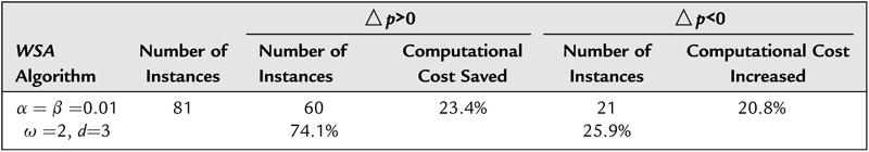
Performances: W. Zhang (1988) uses 8-puzzle as an example to compare the performances of WSA and A. The results are shown in Table 6.1. There are totally 81 instances. The performance of SA is superior to A in 60 instances. Conversely, A is superior to SA only in 21 instances. The computational costs saved are 23.4% and 20.8%, respectively. As we know, 8-puzzle is a problem with a small size. Its longest solution path only contains 35 moves. We can expect that when the problem size becomes larger, SA will demonstrate more superiority.
∗Where, the computational cost-the number of moves,  -significance level,
  -weight, d–when WSA search reaches d (depth) the statistical inference is made, and
  .
.
Table 6.1
The Comparison of Performances between WSA and A
| WSA Algorithm | Number of Instances | ||||
| Number of Instances | Computational Cost Saved | Number of Instances | Computational Cost Increased | ||
| 81 | 60 74.1% | 23.4% | 21 25.9% | 20.8% | |
..................Content has been hidden....................
You can't read the all page of ebook, please click here login for view all page.