
Chapter 11
Machine Learning for Audio
P. Bhattacharya P. Nowak and U. Zölzer
11.1 Introduction
Machine learning can be described as a set of methods or algorithms that offer the capability to learn from data automatically and develop flexible parameterized models. In classical machine learning, the important features of the input are manually designed and extracted from data, and the system automatically learns to map these features to the requisite outputs. This learning is usually achieved through parameter adaptation and/or hyper‐parameter tuning based on a predefined goal or optimization of a cost function. Classical machine learning is used in, and works well for, simple pattern recognition problems. A bulk of the effort or computation would include the design of optimal features for the system. Once the features are handcrafted from a dataset, a generic classification or regression model is used to obtain the output. Some examples of classical machine learning algorithms include linear regression, logistic regression, k‐nearest neighbors, and simple decision trees. Representation learning goes a step further and mostly eliminates the need for handcrafted features. Instead, the required features are automatically discovered from the data. With the evolution of graphical processing units, new machine learning methods supporting more complex models have come to the forefront, with deep learning being one of the major topics of research. Deep learning is part of a broader family of machine learning methods, primarily based on artificial neural networks with representation learning. In deep learning, there are multiple levels of feature extraction from raw or processed data. These features are automatically extracted and combined across various levels to produce the output. Each level can be composed of linear and nonlinear, modifiable, and parameterized operators that can extract and represent features from the representations in the preceding level. With the increment of diverse levels inside the model, the complexity of the overall model increases and helps in an improved fine‐tuned feature representation. Deep learning architectures such as deep neural network (DNN), recurrent neural network (RNN), and convolutional neural network (CNN) have been applied to multiple fields, which include computer vision, audio recognition, natural language processing, social network filtering, machine translation, medical image analysis, material inspection, and gaming. In most of the areas, they have produced much improved results compared to the previous methods.
11.2 Unsupervised and Supervised Learning
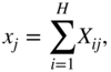
Machine learning algorithms can be primarily classified into supervised, unsupervised, and reinforcement learning, of which the first two methods are of particular interest and are used widely in signal processing applications. Figure 11.1 shows a minimal representation of an unsupervised and a supervised system. Unsupervised learning is a task of identifying previously undetected patterns in a dataset with no labels and with a minimum of human supervision. In contrast to supervised learning that usually makes use of human‐labeled data, unsupervised learning methods primarily extract underlying statistical or semantic features from the input data and allow for modeling of probability densities over inputs. In audio processing, feature extraction across various domains [Ler12] is very important for applications like audio analysis and fingerprinting, decomposition and separation, and content‐based information retrieval [Mül15]. The underlying features or statistics can be analyzed and used to categorize incoming data, identify outliers, or generate latent representations. A clustering method, like the ![]() ‐means algorithm [Mac67] or a mixture model, is a classical unsupervised learning method that groups unlabeled data into categories. It tries to recognize the common features in data and categorizes a new input based on the presence or absence of such features. Hence, such methods can be used in anomaly detection where an input does not belong to any group [Lu16]. Other popular unsupervised methods like the principal component analysis (PCA), independent component analysis (ICA), and non‐negative matrix factorization (NMF) are also used extensively in audio processing and acoustics. ICA is a method which recovers unobserved signals from observed mixtures under the assumption of mutual independence. ICA or its faster variants are used for blind source separation in audio [Chi06] and music classification [Poh06], among others. NMF is another method which has a clustering or grouping property, and is also used for blind source separation [Vir07] and music analysis [Fev09]. Deep unsupervised learning is usually based on deep neural networks without explicit input/label pairs for training. Some models employed in deep unsupervised learning include autoencoder, deep belief network (DBN), and self organizing map (SOM), which are primarily used for dimension reduction or creation of latent variables. SOM is a neural network which produces a low‐dimensional representation of a large input space and is useful for visualization. Autoencoders are used to generate latent variables which could be of a smaller size compared to the original high fidelity input and hence could be used in audio compression [Min19]. However, autoencoders, belief networks, or similar networks can learn underlying latent representations or embeddings from the input data, which can be used for classification tasks. An example of a neural network for speaker verification can be found in [Sny17] where the network learns to create embeddings, named as x‐vectors.
‐means algorithm [Mac67] or a mixture model, is a classical unsupervised learning method that groups unlabeled data into categories. It tries to recognize the common features in data and categorizes a new input based on the presence or absence of such features. Hence, such methods can be used in anomaly detection where an input does not belong to any group [Lu16]. Other popular unsupervised methods like the principal component analysis (PCA), independent component analysis (ICA), and non‐negative matrix factorization (NMF) are also used extensively in audio processing and acoustics. ICA is a method which recovers unobserved signals from observed mixtures under the assumption of mutual independence. ICA or its faster variants are used for blind source separation in audio [Chi06] and music classification [Poh06], among others. NMF is another method which has a clustering or grouping property, and is also used for blind source separation [Vir07] and music analysis [Fev09]. Deep unsupervised learning is usually based on deep neural networks without explicit input/label pairs for training. Some models employed in deep unsupervised learning include autoencoder, deep belief network (DBN), and self organizing map (SOM), which are primarily used for dimension reduction or creation of latent variables. SOM is a neural network which produces a low‐dimensional representation of a large input space and is useful for visualization. Autoencoders are used to generate latent variables which could be of a smaller size compared to the original high fidelity input and hence could be used in audio compression [Min19]. However, autoencoders, belief networks, or similar networks can learn underlying latent representations or embeddings from the input data, which can be used for classification tasks. An example of a neural network for speaker verification can be found in [Sny17] where the network learns to create embeddings, named as x‐vectors.
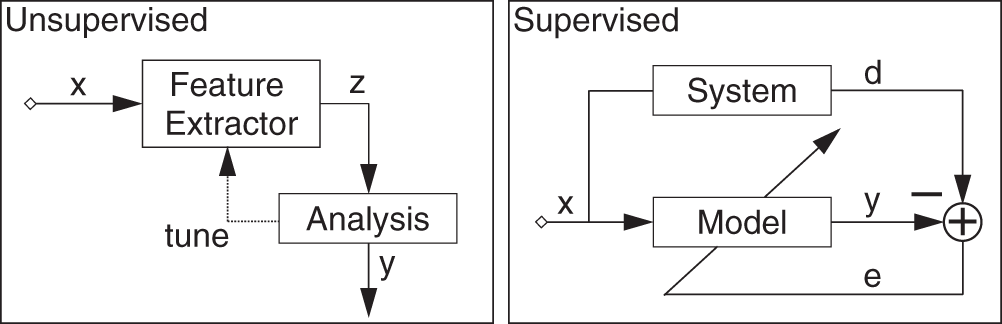
Figure 11.1 A minimal illustration of unsupervised and supervised learning models.
Supervised learning is the task of learning a generalized mapping function of a system based on example input–label pairs. It models a function from labeled training data consisting of a set of examples. In supervised learning, each example is a pair consisting of an input and a desired output value. Supervised models have a predefined cost function that compares the predicted and desired output values. Based on any difference or similarity between the two, the model parameters are iteratively updated with a goal towards minimizing the difference or maximizing the similarity. Linear and logistic regression methods are two of the basic supervised learning methods based on least square minimization or least absolute deviation, and maximum likelihood estimation. These methods and their improved versions are used to estimate model parameters or coefficients to fit a given data or criteria. Other well‐known methods include ![]() ‐nearest neighbors (
‐nearest neighbors (![]() ‐NN) and decision trees, where the latter is used in multiple audio applications [Lav09, Aka12]. Support vector machine (SVM) is another popular learning method mostly used for classification tasks, and it has been applied to perform audio classification and retrieval [GL03, LL01]. Deep learning methods gradually came to the forefront with DNN, CNN, and generative adversarial network (GAN). Deep learning architectures are gradually being used for a variety of audio applications like audio enhancement [Mee18], music recognition [Han17], pitch estimation [Zha16], virtual analog modeling [Mar20] and more.
‐NN) and decision trees, where the latter is used in multiple audio applications [Lav09, Aka12]. Support vector machine (SVM) is another popular learning method mostly used for classification tasks, and it has been applied to perform audio classification and retrieval [GL03, LL01]. Deep learning methods gradually came to the forefront with DNN, CNN, and generative adversarial network (GAN). Deep learning architectures are gradually being used for a variety of audio applications like audio enhancement [Mee18], music recognition [Han17], pitch estimation [Zha16], virtual analog modeling [Mar20] and more.
This chapter is particularly focused on deep learning methods and it illustrates the concept of backpropagation on simple neural and convolutional network architectures, through useful derivations. Additionally, certain example applications are provided to illustrate the usability and performance of these methods in multiple areas of audio processing.
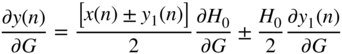
11.3 Gradient Descent and Backpropagation
Most supervised or semi‐supervised machine learning algorithms include an objective function based on a ground truth or a prior, which is usually minimized to find an optimal set of parameters. The consequent derivation from this optimization criteria leads to the method of steepest descent, where the optimal solution is directly proportional to the negative gradient of the objective function. In deep learning, the proposed models are usually multilayered and consist of differentiable parameterized functions. To find the optimal set of parameters, the respective gradients of the objective function with respect to the parameters need to be calculated. The required gradient is eventually broken into a product of multiple local gradients from the hidden layers by the chain rule of derivatives. This method is generally known as backpropagation. The following section describes an artificial neural network (ANN) and exhibits how backpropagation works through the network layers.
11.3.1 Feedforward Artificial Neural Network
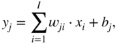
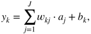
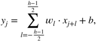
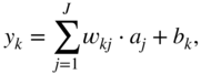
An artificial neural network is based on a collection of connected units or nodes called artificial neurons, which loosely model the neurons in a biological brain. Each connection, like the synapses in a biological brain, can transmit a signal to other neurons. An artificial neuron that receives a signal then processes it and can stimulate the connected neurons. In ANN implementations, the signal at a connection is a real number and the output of each neuron is computed by some nonlinear function of the sum of its inputs. Neurons and their connections typically have a weight that is adapted as learning proceeds. The weight increases or decreases the strength of the signal at a connection. In the case of multilayer perceptrons (MLP) [Ros61], neurons may have a threshold such that a signal is sent or the neuron is fired only if the aggregate surpasses the threshold. Typically, neurons are aggregated into layers and different layers may perform different transformations on their inputs. Signals travel from the first layer, or the input layer, to the last layer, or the output layer, possibly after traversing a number of intermediate layers, also referred to as hidden layers. An example neural network with one hidden layer is illustrated in Fig. 11.2. Every node of one layer is connected to every other node of the succeeding layer by scalar weights, which results in a densely connected structure and a matrix of scalar weights. The dimensions of a weight matrix is defined by the dimensions of the connected layers. Given an input element ![]() , hidden element
, hidden element ![]() , hidden activation
, hidden activation ![]() , and output element
, and output element ![]() , the operations are given by
, the operations are given by
where ![]() and
and ![]() represent the associated scalar weight between
represent the associated scalar weight between ![]() and
and ![]() and the bias, respectively, and
and the bias, respectively, and ![]() and
and ![]() represent the associated scalar weight between
represent the associated scalar weight between ![]() and
and ![]() and the corresponding bias, respectively. Equation (11.2) refers to an activation operation, where
and the corresponding bias, respectively. Equation (11.2) refers to an activation operation, where ![]() refers to a sigmoid activation function described in the next section.
refers to a sigmoid activation function described in the next section.
Activation Function
An activation function performs a nonlinear operation on each neuron individually, retaining the dimensions of that layer. The most commonly used activations in ANN are the sigmoid, Tanh, and the ReLU functions, as illustrated in Fig. 11.3. The sigmoid function is given by
where ![]() is the input to the layer. The derivative of this function is given by
is the input to the layer. The derivative of this function is given by
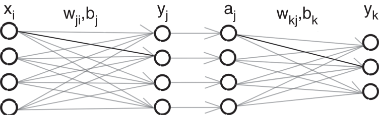
Figure 11.2 A feedforward neural network with one hidden layer.
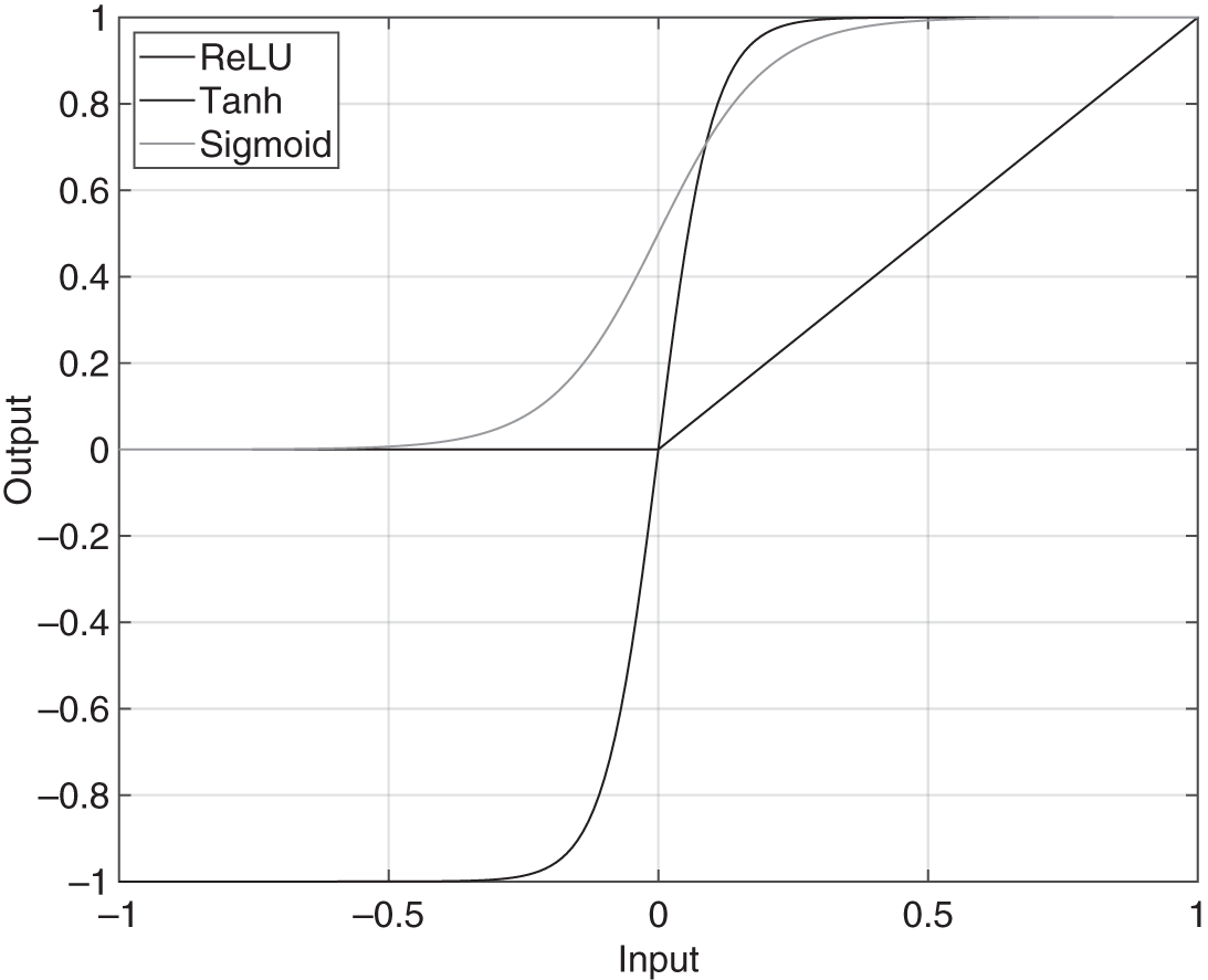
Figure 11.3 Activation functions.
The Tanh function (![]() ) is an activation or gating unit given by
) is an activation or gating unit given by
and its derivative is given by
Rectified linear unit (ReLU) is another activation function, which is given by
having a point of discontinuity at 0. The corresponding approximate derivative is given by
Backpropagation
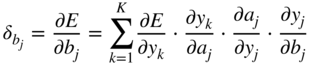
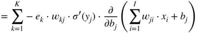
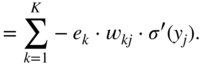
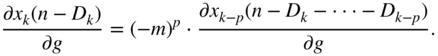
Based on the network shown in Fig. 11.2, the parameter elements ![]() ,
, ![]() , for any
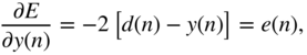
, for any ![]() , need to be updated and the goal is to calculate the corresponding gradients. The loss function is assumed to be a sum of squared error given by
, need to be updated and the goal is to calculate the corresponding gradients. The loss function is assumed to be a sum of squared error given by
where ![]() denotes a ground truth element or label. The gradient
denotes a ground truth element or label. The gradient ![]() , required for updating the weight parameter
, required for updating the weight parameter ![]() , is expressed and extended according to the chain rule of derivatives as
, is expressed and extended according to the chain rule of derivatives as
In a similar way, the gradient ![]() , to update the bias term
, to update the bias term ![]() , is given by
, is given by
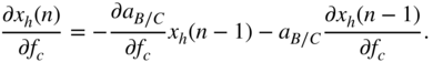
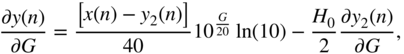
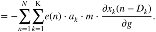
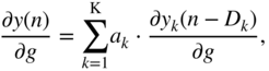
Additionally, the partial gradient of the loss function with respect to the hidden activation ![]() , which will be backpropagated to the previous layer, is given by
, which will be backpropagated to the previous layer, is given by
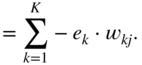
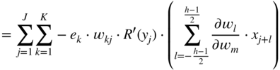
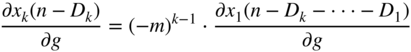
In the next step, it is necessary to calculate the gradient ![]() , required for updating the weight parameter
, required for updating the weight parameter ![]() , and it can be expressed and extended according to the chain rule of derivatives. Assuming that a sigmoid activation is used and with the help of the Eqs. (11.17) and (11.3), it can be derived as
, and it can be expressed and extended according to the chain rule of derivatives. Assuming that a sigmoid activation is used and with the help of the Eqs. (11.17) and (11.3), it can be derived as
The expression ![]() in the above equations is the local derivative of the sigmoid activation function, as given by Eq. (11.5). The gradient
in the above equations is the local derivative of the sigmoid activation function, as given by Eq. (11.5). The gradient ![]() is calculated similarly and is given by
is calculated similarly and is given by
In the next step, the parameters can be iteratively updated with the help of a simple gradient descent, given by
where ![]() and
and ![]() denote the step sizes or learning rates for weights and biases, respectively. The learning rate is usually a small fractional value and
denote the step sizes or learning rates for weights and biases, respectively. The learning rate is usually a small fractional value and ![]() is usually lower than
is usually lower than ![]() . Gradient descent or stochastic gradient descent is usually very slow in convergence when used in a deep learning method across large datasets. Hence, faster gradient descent methods like Nesterov momentum [Nes83], adaptive gradient or adagrad [Duc11], rmsprop [Dau15], and adaptive momentum or adam [Kin15] are primarily used for large‐scale deep learning applications.
. Gradient descent or stochastic gradient descent is usually very slow in convergence when used in a deep learning method across large datasets. Hence, faster gradient descent methods like Nesterov momentum [Nes83], adaptive gradient or adagrad [Duc11], rmsprop [Dau15], and adaptive momentum or adam [Kin15] are primarily used for large‐scale deep learning applications.
11.3.2 Convolutional Neural Network
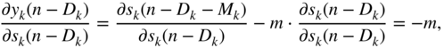
A CNN is an artificial neural network which contains at least one convolutional unit which performs a convolution or cross‐correlation between the input and a set of pre‐defined filters. The filter coefficients, also referred to as weights, are initialized using one of the widely used initialization methods [Glo10, He15] and are subsequently updated iteratively. The primary advantage of such a network over a feedforward artificial neural network is that a convolutional layer contains fewer parameters compared to a corresponding fully connected layer. A CNN also contains hidden layers and an activation function between each convolutional layer. An example network with one hidden layer is illustrated in Fig. 11.4, which contains a convolutional unit and a fully connected unit. The hidden layer is produced by the filtering operation between the nodes in the input layer and the pre‐initialized filters in the convolutional unit. The filtering operation is followed by a ReLU activation function, which is commonly used in a CNN. Finally, the hidden activations are densely connected with the neurons of the output layer. Given an input element ![]() , hidden element
, hidden element ![]() , hidden activation
, hidden activation ![]() , and output element
, and output element ![]() , the operations are given by
, the operations are given by
where ![]() and
and ![]() represent the associated filter coefficient of the filter having a length
represent the associated filter coefficient of the filter having a length ![]() and the scalar bias value, respectively, and
and the scalar bias value, respectively, and ![]() and
and ![]() represent the associated scalar weights between
represent the associated scalar weights between ![]() and
and ![]() and the corresponding bias, respectively. The convolutional unit can also contain multiple filters and bias values resulting in a hidden layer containing multiple stacked vectors instead of one vector.
and the corresponding bias, respectively. The convolutional unit can also contain multiple filters and bias values resulting in a hidden layer containing multiple stacked vectors instead of one vector.
Figure 11.4 A convolutional neural network with one hidden layer.
Based on the network shown in Fig. 11.4, the weight elements ![]() ,
, ![]() , and
, and ![]() need to be updated and the goal is to calculate the corresponding gradients. The gradient
need to be updated and the goal is to calculate the corresponding gradients. The gradient ![]() , required for updating the weight parameter
, required for updating the weight parameter ![]() , is already given by Eq. (11.13) while the gradient
, is already given by Eq. (11.13) while the gradient ![]() , to update the bias term
, to update the bias term ![]() , is given by Eq. (11.14). Additionally, the partial gradient of the loss function with respect to the hidden activation
, is given by Eq. (11.14). Additionally, the partial gradient of the loss function with respect to the hidden activation ![]() , which will be backpropagated to the previous layer, is given by Eq. (11.17). In the next step, it is necessary to calculate the gradient
, which will be backpropagated to the previous layer, is given by Eq. (11.17). In the next step, it is necessary to calculate the gradient ![]() , required for updating the filter coefficient
, required for updating the filter coefficient ![]() , and it can be expressed and extended according to the chain rule of derivatives. With the help of Eqs. (11.17) and (11.30), it can be derived as
, and it can be expressed and extended according to the chain rule of derivatives. With the help of Eqs. (11.17) and (11.30), it can be derived as
where the expression ![]() is given by
is given by
and the expression ![]() refers to the local derivative of the ReLU activation function, as given by Eq. (11.9). Equation (11.34) leads to a cross‐correlation operation between the incoming gradient and the input vector. The gradient
refers to the local derivative of the ReLU activation function, as given by Eq. (11.9). Equation (11.34) leads to a cross‐correlation operation between the incoming gradient and the input vector. The gradient ![]() is calculated similarly and is given by
is calculated similarly and is given by

After the calculation of the required gradients, the parameters are updated by stochastic gradient descent or a faster parameter update algorithm.
11.4 Applications
The following sections describe several deep learning applications in the area of audio signal processing. In the first example, the application proposed in [Bha20] is described, where a cascade of parametric peak and shelving filters is adapted to model head‐related transfer functions. The iterative optimization method is sample based and uses the instantaneous backpropagation method. In the second example, the sparse feedback delay network (FDN) with Schroeder allpass filters, described in Section 7.3.3, is adapted to model a desired room impulse response or simulate a room impulse response (RIR) based on a desired reverberation time. The final application of the section describes a CNN which is used to reduce Gaussian noise in audio or speech signals.
11.4.1 Parametric Filter Adaptation
Parametric peak and shelving filters, as introduced in Section 6.2.2, can be cascaded to perform audio processing tasks like equalization, spectral shaping, and modeling of complex transfer functions. An independent optimization of the mentioned parameters of each individual filter in this cascaded structure can be performed with the help of a backpropagation algorithm. Earlier research in this area includes the work done in [Gao92], which introduces a backpropagation‐based adaptive IIR filter, and in [Ros99], which trained a recursive filter with derivative function to adapt a controller. In the context of neural networks, a cascaded structure of FIR and IIR filters with multilayer perceptrons was used in [Bac91] for time‐series modeling based on a simplified instantaneous backpropagation through time (IBPTT). A similar adaptive IIR‐multilayer perceptron (IIR‐MLP) network was also described in [Cam96] based on causal backpropagation through time (CBPTT). In recent years, backpropagation is extensively used in CNNs as well as recurrent neural networks, the latter being recursive in nature. However, in the aforementioned literature, the adaptation is primarily performed directly on filter coefficients. This work is one of the few methods that adapt the control parameters with deep learning [Ner20, Väl19, Eng20] and the application described in this section is already introduced in [Bha20].
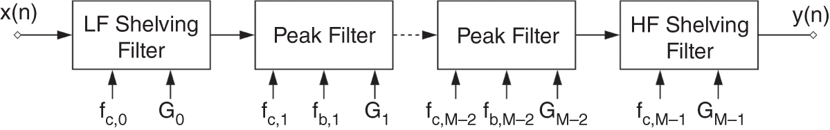
Figure 11.5 A cascaded structure of peak and shelving filters.
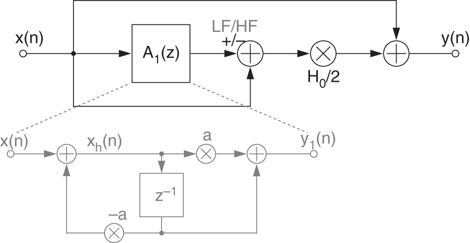
Figure 11.6 Signal flow graph of a LF/HF shelving filter.
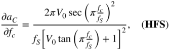
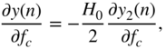
The proposed cascaded structure with M filters is illustrated in Fig. 11.5, where the first and the last filters are shelving filters while the remaining filters are peak filters. Peak and shelving filters are described in Section 6.2.2 along with their illustrations and transfer functions. From the transfer functions defining low‐frequency and high‐frequency shelving filters (LFS and HFS) in Eq. (6.59) and Eq. (6.71), one can derive the signal flow graph in Fig. 11.6 and the corresponding difference equation can be calculated to be
where ![]() defines the output signal of a first‐order allpass filter according to
defines the output signal of a first‐order allpass filter according to
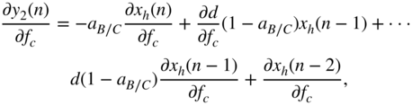
Similarly, the signal flow graph in Fig. 11.7 and the difference equation of a peak filter can be derived from Eq. (6.81) as
where ![]() defines the output signal of a second‐order allpass filter according to
defines the output signal of a second‐order allpass filter according to
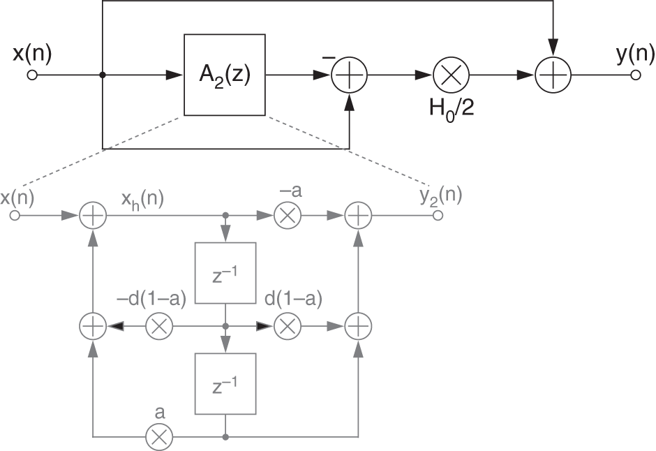
Figure 11.7 Signal flow graph of a peak filter.
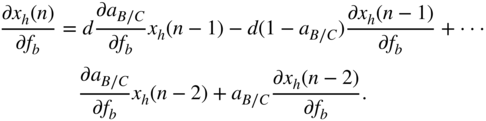
The partial derivative of a pre‐defined cost function, with respect to the filter parameters in a cascaded structure, needs to be calculated as a product of multiple local derivatives according to the chain rule. Given the cascaded structure and a reference system under test, a global instantaneous cost or loss function ![]() for the
for the ![]() th sample can be defined, as shown in Fig. 11.8. The derivative of the cost function with respect to a parameter
th sample can be defined, as shown in Fig. 11.8. The derivative of the cost function with respect to a parameter ![]() can be written as
can be written as
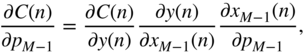
according to the chain rule of derivatives, where ![]() represents the predicted output of the cascaded filter structure,
represents the predicted output of the cascaded filter structure, ![]() represents the desired output of the system under test,
represents the desired output of the system under test, ![]() represents the output of the {
represents the output of the {![]() }th filter in the cascade, and
}th filter in the cascade, and ![]() represents any control parameter like gain, bandwidth, or center frequency of the {
represents any control parameter like gain, bandwidth, or center frequency of the {![]() }th peak filter.
}th peak filter.
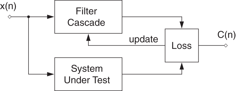
Figure 11.8 Block diagram of the model.
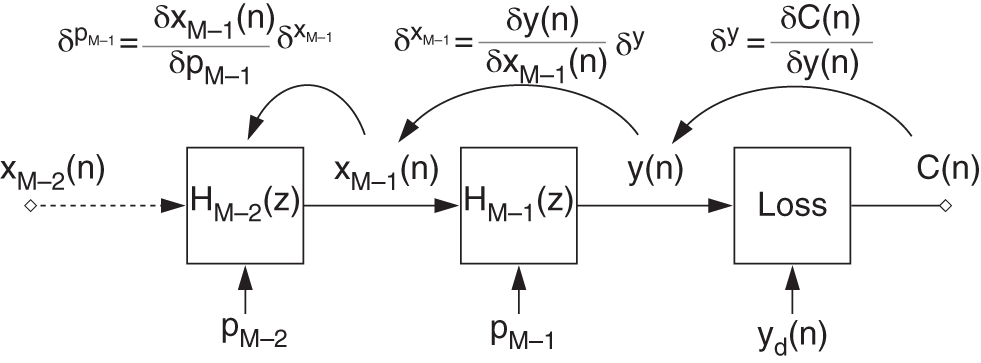
Figure 11.9 Illustration of backpropagation through the cascaded structure.
This will result in a simplified instantaneous backpropagation algorithm [Bac91], which is illustrated in Fig. 11.9. To calculate the above derivative, with respect to the instantaneous cost function, it is necessary to calculate the local derivative ![]() of the cost function, the local derivative
of the cost function, the local derivative ![]() of a filter output with respect to its input, and the local derivative
of a filter output with respect to its input, and the local derivative ![]() of a filter output with respect to its parameter
of a filter output with respect to its parameter ![]() . Hence, in general, the above three types of local gradients need to be calculated to adapt the cascaded structure. In the following sections, the local gradients of the filter output against the filter input and the control parameters are derived for shelving and peak filters. Finally, the cascaded structure is used for modeling head‐related transfer function (HRTF) magnitudes as an example application.
. Hence, in general, the above three types of local gradients need to be calculated to adapt the cascaded structure. In the following sections, the local gradients of the filter output against the filter input and the control parameters are derived for shelving and peak filters. Finally, the cascaded structure is used for modeling head‐related transfer function (HRTF) magnitudes as an example application.
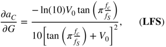
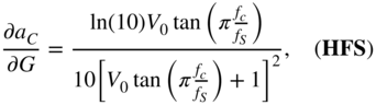
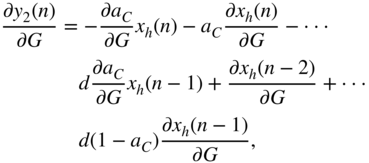
Shelving Filter
For a shelving filter, local derivatives of the filter output are calculated against the filter input, the gain, and the cutoff frequency. Referring to Eq. (11.38), the derivative of a low‐frequency shelving (LFS) and a high‐frequency shelving (HFS) filter output ![]() , with respect to its input
, with respect to its input ![]() , is calculated as
, is calculated as

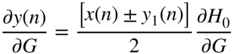
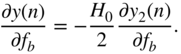
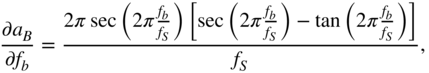
The derivative of the shelving filter output, with respect to the filter gain ![]() , for the boost case is calculated as
, for the boost case is calculated as

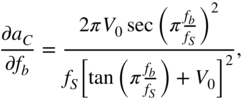
The derivative of the filter output, with respect to the filter gain ![]() , for the cut case is different from the boost case because of the dependence between the gain parameter and the parameter for cutoff frequency that can be seen in Eqs. (6.47) and (6.53). With the help of Eq. (11.38), it can calculated as
, for the cut case is different from the boost case because of the dependence between the gain parameter and the parameter for cutoff frequency that can be seen in Eqs. (6.47) and (6.53). With the help of Eq. (11.38), it can calculated as
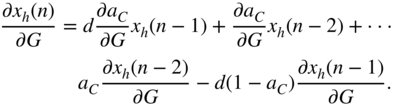
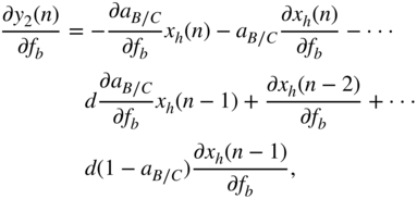
where the expression ![]() of Eq. (11.50) can be extended with the help of Eq. (11.39) as
of Eq. (11.50) can be extended with the help of Eq. (11.39) as
with
From Eq. (11.54), ![]() is calculated by employing the chain rule of derivatives and IBPTT with the initialization of
is calculated by employing the chain rule of derivatives and IBPTT with the initialization of ![]() .
.
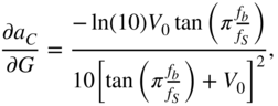
Finally, the derivative of the shelving filter output, with respect to the cutoff frequency ![]() , is calculated as
, is calculated as
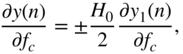
where
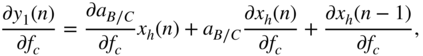
with
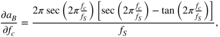
From Eq. (11.60), ![]() is calculated by employing the chain rule of derivatives and IBPTT with the initialization of
is calculated by employing the chain rule of derivatives and IBPTT with the initialization of ![]() .
.
Peak Filter
For a peak filter, local derivatives of the filter output are calculated against the filter input, the gain, the center frequency, and the bandwidth. Referring to Eq. (11.41), the derivative of a second‐order peak filter output ![]() , with respect to its input
, with respect to its input ![]() , is calculated as
, is calculated as
As done in the case of shelving filters, the derivative of the peak filter output, with respect to the filter gain ![]() , for the boost case will result in
, for the boost case will result in
For the cut case as well, the derivative of the peak filter output, with respect to the filter gain ![]() , is derived in a similar manner. With the help of Eq. (11.41), the derivation leads to
, is derived in a similar manner. With the help of Eq. (11.41), the derivation leads to
and the expression ![]() from the above equation can be extended with the help of Eq. (11.42) as
from the above equation can be extended with the help of Eq. (11.42) as
with
and
From Eq. (11.66), the expressions ![]() and
and ![]() are calculated with the chain rule of derivatives and IBPTT with the initialization of
are calculated with the chain rule of derivatives and IBPTT with the initialization of ![]() and
and ![]() .
.
The derivative of the peak filter output, with respect to the cutoff frequency ![]() , leads to an expression similar to Eq. (11.55) given by
, leads to an expression similar to Eq. (11.55) given by
where
with
and
From Eq. (11.70), the expressions ![]() and
and ![]() are calculated with the chain rule of derivatives and IBPTT with the initialization of
are calculated with the chain rule of derivatives and IBPTT with the initialization of ![]() and
and ![]() .
.
Finally, the derivative of the peak filter output, with respect to the bandwidth ![]() , is calculated as
, is calculated as
From the above equation, ![]() is calculated as
is calculated as
with
and
From Eq. (11.75), the expressions ![]() and
and ![]() are calculated with chain rule of derivatives and IBPTT with the initialization of
are calculated with chain rule of derivatives and IBPTT with the initialization of ![]() and
and ![]() .
.
Cascaded Structure
With the help of the above formulations, the necessary gradients for parameter update can be derived. As an example, the derivative of the cost function, e.g. the squared‐error function given by
with respect to the gain of the {![]() }th peak filter
}th peak filter ![]() in the filter cascade, as shown in Fig. 11.9, is given by
in the filter cascade, as shown in Fig. 11.9, is given by
according to Eq. (11.44). If the boost case is assumed, then with the help of the derivative of the cost function from Eq. (11.76), with respect to ![]() given by
given by
Eq. (11.61), and Eq. (11.62), the required gradient for parameter update is derived as
where
The gain ![]() is subsequently updated by the above expression, preferably with the adaptive momentum update for faster convergence.
is subsequently updated by the above expression, preferably with the adaptive momentum update for faster convergence.
Head‐related Transfer Function Modeling
An HRTF is a direction dependent transfer function between an external sound source and the human ear. The inverse Fourier transform of the HRTF is the head‐related impulse response (HRIR). In spatial audio through headphones, mono signals are filtered with the corresponding HRIRs to create a virtual sound that is localized in a certain direction. To achieve a good resolution of the 3‐D space, HRIRs have to be saved for a high number of directions, which results in a large amount of stored data. Hence, parametric IIR filters can be used to model the HRTF magnitudes with a lower number of saved parameters.
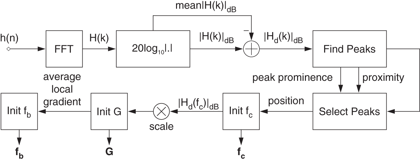
Figure 11.10 Block diagram illustrating the initialization method for HRTF modeling.

Figure 11.11 Magnitude responses: in the top plot, the whole filter cascade; and in the bottom plot, all individual filter stages of the desired HRTF, the initial HRTF estimate, and the final approximation of the right ear of ‘Subject‐008’, for an azimuth  and elevation
  .
.
For the initialization of the cascaded filter structure, an approximated number of required peak filters needs to be determined. Afterward, the allocation of the initial parameter values is done, as illustrated in Fig. 11.10. Initially, the magnitude response is smoothed and the mean of the magnitude response is subtracted. Based on the prominence and proximity to one another, a finite number of peaks and notches are selected. The initial center frequency of a peak filter is determined based on the position of a peak or notch while the initial cutoff frequencies of the shelving filters are determined based on the slopes in the magnitude response. The gain of a filter is initialized by the magnitude of the transfer function at the position of the peak or notch. To reduce the summation effect arising from the cascade, the gain of every peak filter is scaled by a fractional factor depending on the magnitude. Gains of notches in the positive half and peaks in the negative half are converted to small negative and positive values, respectively. Finally, the bandwidth of a peak filter is initialized based on the average local gradient of the magnitude response around the peak's position. The number of filters can be reduced or increased based on the third step. A major drawback of such an initialization is that more than an optimal number of filters will usually be proposed. Additionally, the peak picking method will be insufficient in flat regions. However, a direct initialization is simple and the simultaneous filter update improves the run‐time.
To adapt the cascaded structure, a log‐spectral distance between the estimated and the desired magnitude responses is considered as the objective function, which is given by
where ![]() and
and ![]() denote the magnitude responses of the desired and estimated output signals, respectively, in dB, and
denote the magnitude responses of the desired and estimated output signals, respectively, in dB, and ![]() denotes a frequency bin. The derivative of the Fourier transform between time and frequency domain can be performed with the help of Wirtinger calculus, as demonstrated in [Car17] and [Wan20].
denotes a frequency bin. The derivative of the Fourier transform between time and frequency domain can be performed with the help of Wirtinger calculus, as demonstrated in [Car17] and [Wan20].
For the evaluation, a subset of HRIRs from the CIPIC database [Alg01] is chosen to evaluate the HRTF magnitude approximation. In the first step, the HRIRs are converted to HRTFs and the magnitude responses are treated as the desired signal for the filter cascade. Nevertheless, before performing the discrete Fourier transform, the HRIRs are padded with zeros to a length of 1024 to achieve a better frequency resolution. Afterward, the aforementioned initialization is performed. Owing to differences in the HRTFs between subjects and directions, every transfer function needs a unique initialization, which can result in a different number of peak filters and initial parameter values. After the initialization of the cascaded structure, the filters are trained and updated for 100 epochs with the adam method [Kin15]. However, in the cases of most HRTFs, a smaller number of epochs is sufficient to achieve a good approximation. The learning rate during the update method is selected as ![]() . Additionally, there is a learning rate drop factor of 0.99 for every time the error in a particular epoch is higher than the error in the previous epoch. The aforementioned hyper‐parameters might change for a few exceptional cases where convergence requires different values.
. Additionally, there is a learning rate drop factor of 0.99 for every time the error in a particular epoch is higher than the error in the previous epoch. The aforementioned hyper‐parameters might change for a few exceptional cases where convergence requires different values.
In Fig. 11.11, the magnitude responses of the desired HRTF, the initial HRTF estimate, and the final approximation of the right ear of ‘Subject_008’, for an azimuth ![]() and elevation
and elevation ![]() , are plotted. As can be seen, the algorithm is able to reproduce the desired magnitude response with 17 peaks and two shelving filters. A more detailed evaluation and discussion can be found in [Bha20].
, are plotted. As can be seen, the algorithm is able to reproduce the desired magnitude response with 17 peaks and two shelving filters. A more detailed evaluation and discussion can be found in [Bha20].
11.4.2 Room Simulation
In the following application, a sparse FDN, introduced in Section 7.3.3, is adapted to simulate a desired RIR. This section provides some derivations related to the proposed FDN with a cascaded allpass filter and delay line in each of the ![]() branches having a sparse diagonal feedback matrix. Figure 11.12 shows an overview of the proposed FDN. The corresponding difference equations are given as
branches having a sparse diagonal feedback matrix. Figure 11.12 shows an overview of the proposed FDN. The corresponding difference equations are given as
where ![]() denotes the overall output of the network,
denotes the overall output of the network, ![]() denotes the
denotes the ![]() th coefficient of a mixing vector,
th coefficient of a mixing vector, ![]() denotes the output of the
denotes the output of the ![]() th Schroeder allpass,
th Schroeder allpass, ![]() and
and ![]() denote the associated delays inside the allpass and the subsequent delay line of the
denote the associated delays inside the allpass and the subsequent delay line of the ![]() th branch, respectively,
th branch, respectively, ![]() denotes a state of the
denotes a state of the ![]() th Schroeder allpass,
th Schroeder allpass, ![]() denotes the input to the
denotes the input to the ![]() th Schroeder allpass,
th Schroeder allpass, ![]() denotes the input signal to the overall network, and
denotes the input signal to the overall network, and ![]() ,
, ![]() are the control parameters. The output of the FDN is sent to a loss function given by
are the control parameters. The output of the FDN is sent to a loss function given by
where ![]() denotes the desired signal that works as a ground truth or label. To adapt
denotes the desired signal that works as a ground truth or label. To adapt ![]() , the expression
, the expression ![]() should be calculated with chain rule of derivatives and backpropagation as given by
should be calculated with chain rule of derivatives and backpropagation as given by
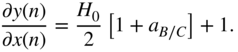
In Eq. (11.89), the following expressions are substituted as
while the following expressions from Eq. (11.91) are given by
From Eq. (11.92), the expression ![]() can be derived further and has to be expressed in the form of
can be derived further and has to be expressed in the form of ![]() , because
, because ![]() is a function of
is a function of ![]() . With the help of Eq. (11.85) the derivation can be written as
. With the help of Eq. (11.85) the derivation can be written as

The expression in Eq. (11.100) can be extended and expressed in a more general form given by
With ![]() , the expression in the above equations can be expressed as a partial derivative function of
, the expression in the above equations can be expressed as a partial derivative function of ![]() , differentiable with respect to
, differentiable with respect to ![]() , and is given by
, and is given by

The second expression in Eq. (11.103) can be extended further and can be neglected for a large ![]() because
because ![]() is usually a small fraction. Combining Eq. (11.92) and Eq. (11.103) will lead to the approximate expression given by
is usually a small fraction. Combining Eq. (11.92) and Eq. (11.103) will lead to the approximate expression given by
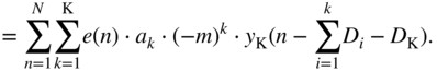
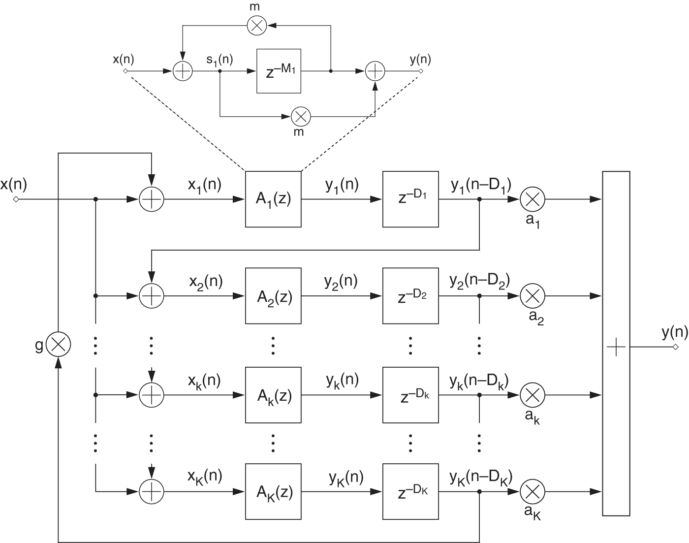
Figure 11.12 Feedback delay network.
In addition to controlling ![]() , the parameters
, the parameters ![]() of the mixing vectors can also be adapted and the expression
of the mixing vectors can also be adapted and the expression ![]() needs to be derived. This derivation is given by
needs to be derived. This derivation is given by
Finally, the respective updates could be performed with gradient descent as
where ![]() and
and ![]() are the respective learning rates and
are the respective learning rates and ![]() is usually chosen as a very small fraction compared with
is usually chosen as a very small fraction compared with ![]() .
.
The update can occur for a finite number of iterations or it can stop based on a minimum error threshold. Instead of a desired RIR, the optimization can also be driven by an approximate desired energy decay curve (EDC) of an impulse response. A normalized EDC for an impulse response ![]() in a discrete case is defined as
in a discrete case is defined as
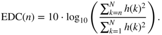
The EDC is used for estimating the reverberation times such as ![]() , and for a long RIR, it decays almost linearly before it subsides rapidly near the end. Hence, in the absence of a desired RIR, a normalized EDC can be constructed based on a desired reverberation time with the assumption of linearity, and this approximate EDC can be used as a ground truth. In this simulation, the input
, and for a long RIR, it decays almost linearly before it subsides rapidly near the end. Hence, in the absence of a desired RIR, a normalized EDC can be constructed based on a desired reverberation time with the assumption of linearity, and this approximate EDC can be used as a ground truth. In this simulation, the input ![]() is an impulse and therefore the estimated output
is an impulse and therefore the estimated output ![]() is an impulse response. The EDC of
is an impulse response. The EDC of ![]() is then calculated and its deviation from the approximate ground truth is used as an error to drive the FDN parameter adaptation. The mixing coefficients
is then calculated and its deviation from the approximate ground truth is used as an error to drive the FDN parameter adaptation. The mixing coefficients ![]() are initialized randomly and scaled, while the initial value of the parameter
are initialized randomly and scaled, while the initial value of the parameter ![]() is selected as 0.3.
is selected as 0.3.
Figure 11.13 shows a simple example of a simulation based on a desired RIR as the ground truth. The first plot shows the normalized decay curves for the final estimated impulse response after 20 iterations, the desired or ground truth impulse response, and the initial impulse response. The second plot shows the final RIR, which is broadband in nature. The EDC indicates a ![]() reverberation time of approximately 0.67 seconds and the density of the impulse response depends on the number of branches in the network. In this simulation, the respective delays inside the allpass filters are purely prime numbers, in terms of number of samples, and they are selected as
reverberation time of approximately 0.67 seconds and the density of the impulse response depends on the number of branches in the network. In this simulation, the respective delays inside the allpass filters are purely prime numbers, in terms of number of samples, and they are selected as ![]() and
and ![]() . If the value of
. If the value of ![]() is very high, a subset of prime values between
is very high, a subset of prime values between ![]() and
and ![]() is selected to reduce the number of branches and accelerate convergence. However, reducing the number of branches leads to a reduction of impulse response density. The delay after an allpass filter is selected as
is selected to reduce the number of branches and accelerate convergence. However, reducing the number of branches leads to a reduction of impulse response density. The delay after an allpass filter is selected as ![]() .
.
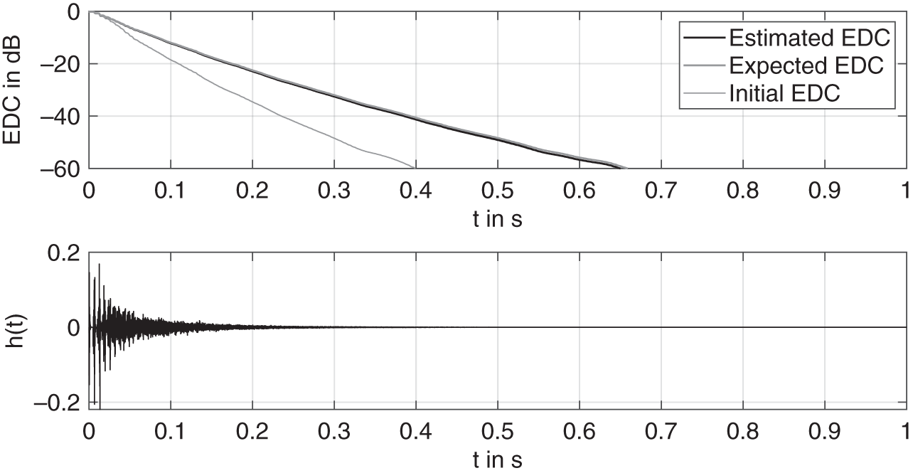
Figure 11.13 Results, in terms of energy decay curves (EDCs) and the final estimated RIR of a room simulation by the FDN based on a desired RIR as ground truth.
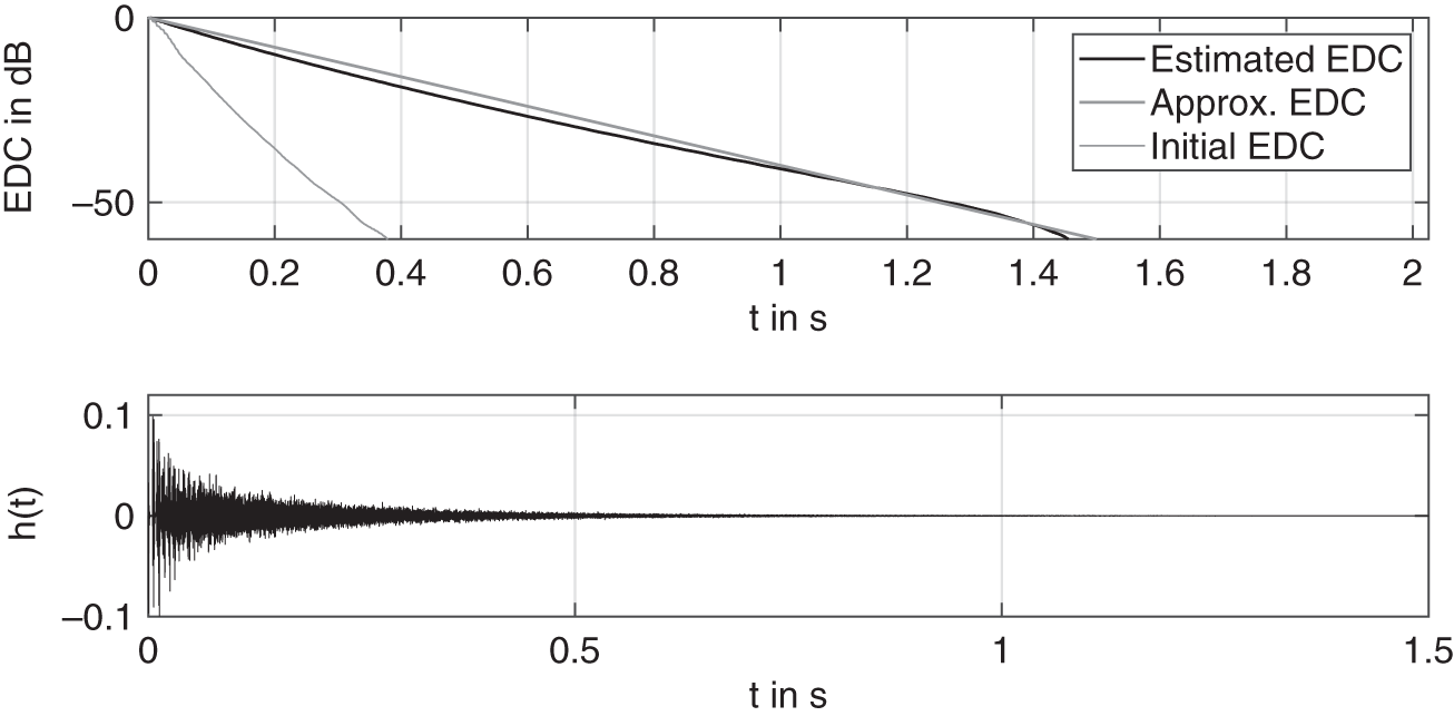
Figure 11.14 Results in terms of EDCs and the final estimated RIR of a room simulation by the FDN based on a desired reverberation time  as ground truth.
Figure 11.14 shows an example of a simulation based on a desired ![]() . The ground truth is created by a linear interpolation on the basis of the proposed
. The ground truth is created by a linear interpolation on the basis of the proposed ![]() as
as ![]() s and is treated as an approximation of the expected EDC. It is however noteworthy that such an approximation of the ground truth is not entirely well posed, owing to its dissimilarity with real EDCs near the tail end. Through the iterations, the EDC of the estimated impulse response gradually drifts towards the approximated ground truth and can eventually improve further. The corresponding final impulse response after 10 iterations is also shown in the plot. The method can be extended to stereo by adding an additional mixing vector of coefficients. A pseudo‐random initialization of each mixing vector ensures that the individual impulse responses are decorrelated to avoid a narrow sound field while rendering an audio or they can be decorrelated during adaptation, if required.
s and is treated as an approximation of the expected EDC. It is however noteworthy that such an approximation of the ground truth is not entirely well posed, owing to its dissimilarity with real EDCs near the tail end. Through the iterations, the EDC of the estimated impulse response gradually drifts towards the approximated ground truth and can eventually improve further. The corresponding final impulse response after 10 iterations is also shown in the plot. The method can be extended to stereo by adding an additional mixing vector of coefficients. A pseudo‐random initialization of each mixing vector ensures that the individual impulse responses are decorrelated to avoid a narrow sound field while rendering an audio or they can be decorrelated during adaptation, if required.
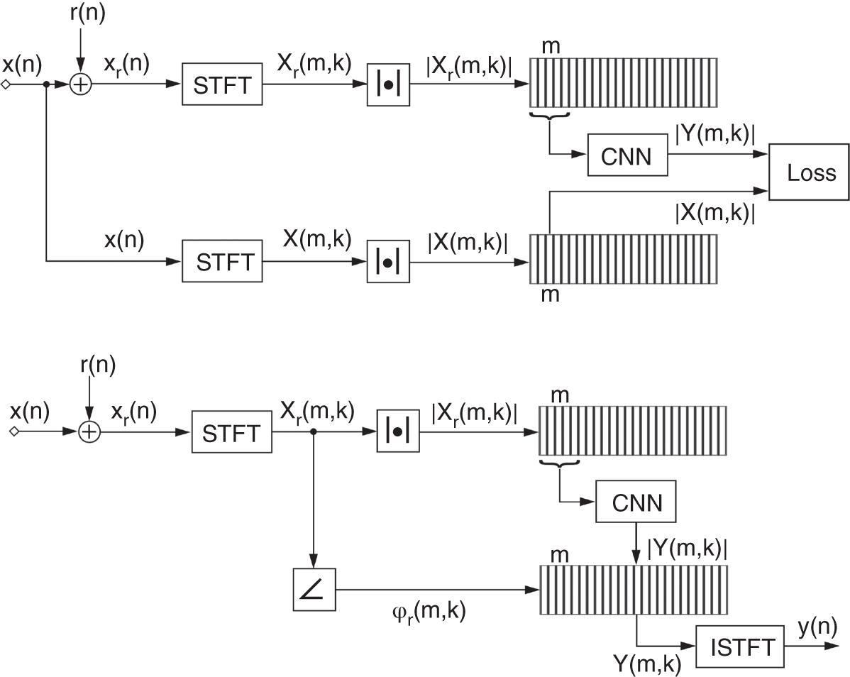
Figure 11.15 Illustration of the denoising model during training phase (top plot) and the testing phase (bottom plot).
11.4.3 Audio Denoising
Noise reduction is one of the most widely performed low level applications in audio signal processing. One of the earliest approaches in noise reduction is the method of spectral subtraction [Bol79], which is quite fast and is suitable for reducing stationary noise. Another popular approach to noise reduction is Wiener filtering based on minimum mean squared error, where an estimation of the a priori signal‐to‐noise ratio (SNR) is required [EM84]. Other methods based on adaptive filtering [Tak03], wavelets [Soo97], adaptive time‐frequency block thresholding [Yu08], and statistical modeling [God01] are proposed for efficient audio restoration. Additionally, companding based noise reduction employed by Dolby and dynamic noise limiters introduced by Philips are some of the commercially used denoising systems. In recent years, deep learning methods have been successfully used in audio denoising and notable deep neural network architectures like CNN [Par17], wavenet [Ret18], and recurrent neural network (RNN) [Val18] have shown very promising results. In this section, a convolutional neural network model is described for an offline audio denoising application against additive Gaussian noise.
Denoising Model
Figure 11.15 illustrates the proposed denoising model. In the training phase, Gaussian noise, denoted by ![]() , is initially added to the clean audio signal sampled at
, is initially added to the clean audio signal sampled at ![]() kHz and denoted by
kHz and denoted by ![]() . It is ensured that the overall SNR in each audio file is
. It is ensured that the overall SNR in each audio file is ![]() dB. The noisy audio is transformed with a short‐time Fourier transform (STFT) using a hamming window of 1024 samples,
dB. The noisy audio is transformed with a short‐time Fourier transform (STFT) using a hamming window of 1024 samples, ![]() % overlap, and a frequency resolution of
% overlap, and a frequency resolution of ![]() Hz. After the transform, its magnitude response is calculated, and the coefficients are normalized between 0 and 1. With a unit stride, consecutive coefficient vectors of the magnitude response, denoted by
Hz. After the transform, its magnitude response is calculated, and the coefficients are normalized between 0 and 1. With a unit stride, consecutive coefficient vectors of the magnitude response, denoted by ![]() and centered around the
and centered around the ![]() th frame, are concatenated along the depth to produce a sequential input for the CNN. The model predicts the denoised coefficient vector of the magnitude response, denoted by
th frame, are concatenated along the depth to produce a sequential input for the CNN. The model predicts the denoised coefficient vector of the magnitude response, denoted by ![]() , while the corresponding magnitude response from the clean audio, denoted by
, while the corresponding magnitude response from the clean audio, denoted by ![]() , is used as the ground truth. The CNN is trained for several epochs with a combination of quadratic loss functions. In the testing phase, the aforementioned data pre‐processing is performed for the test audio and the trained model is used to estimate the denoised magnitude response. The phase response of the noisy audio is then combined with this magnitude response and the inverse STFT is performed to reconstruct the denoised audio signal.
, is used as the ground truth. The CNN is trained for several epochs with a combination of quadratic loss functions. In the testing phase, the aforementioned data pre‐processing is performed for the test audio and the trained model is used to estimate the denoised magnitude response. The phase response of the noisy audio is then combined with this magnitude response and the inverse STFT is performed to reconstruct the denoised audio signal.
Network Architecture
The CNN has a feedforward architecture with inception and attention modules, as illustrated in Fig. 11.16. The input structure contains five consecutive vectors of 513 coefficients each, centered on the ![]() th frame index and it is sent to an inception module [Sze15] containing three parallel convolution layers. The filter groups in the layers have a spatial dimension of
th frame index and it is sent to an inception module [Sze15] containing three parallel convolution layers. The filter groups in the layers have a spatial dimension of ![]() but different dilation factors of 0, 1, and 2, and they produce output feature maps with depths of 32, 16, and 16, respectively. Dilation of a filter refers to the insertion of zeros in between filter coefficients. This ensures that there is an increment in its receptive field but not in the number of training parameters. Multiple dilation factors help in aggregating multiresolution features, which improves the network performance. The padding is adjusted according to the dilation factors and filter sizes so that the output feature maps have the same spatial dimensions. The features generated by the parallel convolutional layers are concatenated along depth to create an output of 64 feature maps, and it is rectified by the ReLU layer. These feature maps are sent to a residual inception‐attention block which features the aforementioned inception module containing an additional batch normalization operation after each convolution layer, and the inception module is followed by an attention module. The attention mechanism was introduced as an improvement in neural machine translation system [Bah15]. Although the mechanism is primarily used in RNNs or LSTMs for natural language processing [Che16], attention has emerged as an important module in computer vision [Xu15] and audio processing [Hao19].
but different dilation factors of 0, 1, and 2, and they produce output feature maps with depths of 32, 16, and 16, respectively. Dilation of a filter refers to the insertion of zeros in between filter coefficients. This ensures that there is an increment in its receptive field but not in the number of training parameters. Multiple dilation factors help in aggregating multiresolution features, which improves the network performance. The padding is adjusted according to the dilation factors and filter sizes so that the output feature maps have the same spatial dimensions. The features generated by the parallel convolutional layers are concatenated along depth to create an output of 64 feature maps, and it is rectified by the ReLU layer. These feature maps are sent to a residual inception‐attention block which features the aforementioned inception module containing an additional batch normalization operation after each convolution layer, and the inception module is followed by an attention module. The attention mechanism was introduced as an improvement in neural machine translation system [Bah15]. Although the mechanism is primarily used in RNNs or LSTMs for natural language processing [Che16], attention has emerged as an important module in computer vision [Xu15] and audio processing [Hao19].
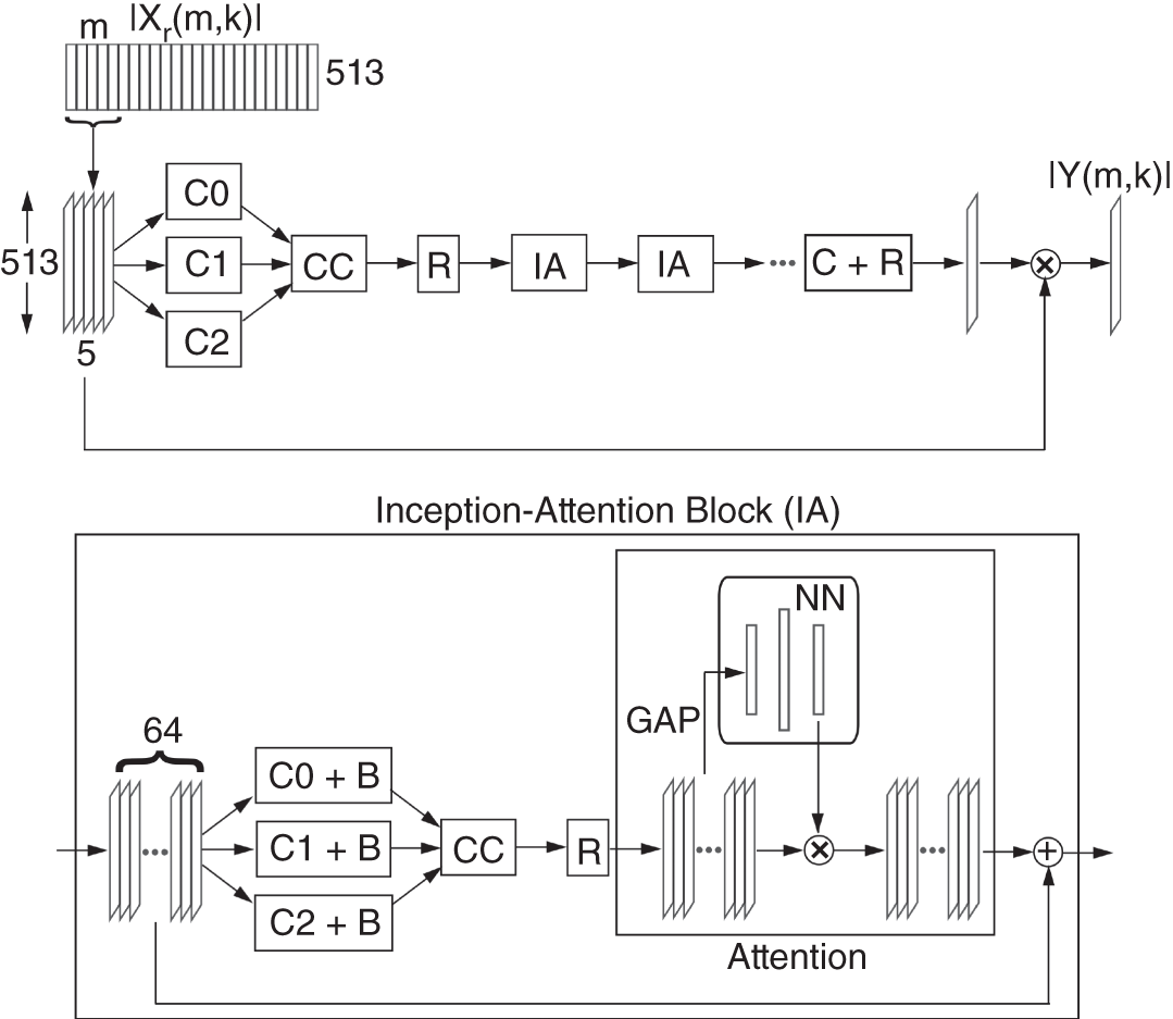
Figure 11.16 Illustration of the CNN architecture, where C0, C1, and C2 denote convolution layers with filter sizes of  ,
,  , and
, and 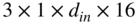 and dilation factors of
  ,
,  , and
, and  , respectively, C denotes a convolution layer with filter size of
 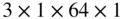 , R denotes a ReLU activation, CC denotes concatenation, BN denotes batch normalization, GAP denotes global average pooling, and NN denotes a neural network.
In the current CNN, a simple self‐attention mechanism is used. At the beginning of this module, a global average pooling is performed across each feature map of the incoming three‐dimensional input, and the operation is given by
where ![]() denotes the
denotes the ![]() th element in the
th element in the ![]() th feature map,
th feature map, ![]() denotes the corresponding scalar output, and
denotes the corresponding scalar output, and ![]() denotes the height of the feature map while its width is 1. Pooling on every feature map of the tensor results in an output vector which is processed by a simple neural network with 1 hidden layer and ReLU activation function. At the output of the neural network, a sigmoid function, given by Eq. (11.4), is used to limit the values between 0 and 1. As an alternative, a softmax function can also be used to get a normalized output vector. Finally, each coefficient of this vector acts as an independent multiplier to tune each feature map of the incoming three‐dimensional structure.
denotes the height of the feature map while its width is 1. Pooling on every feature map of the tensor results in an output vector which is processed by a simple neural network with 1 hidden layer and ReLU activation function. At the output of the neural network, a sigmoid function, given by Eq. (11.4), is used to limit the values between 0 and 1. As an alternative, a softmax function can also be used to get a normalized output vector. Finally, each coefficient of this vector acts as an independent multiplier to tune each feature map of the incoming three‐dimensional structure.
A series of inception–attention blocks are cascaded before a final convolution and ReLU layer which estimates a spectral mask, and the mask is multiplied by the input coefficient vector corresponding to the ![]() th frame to suppress noise. The result is sent to the loss layer where the error is calculated with respect to the ground truth coefficient vector.
th frame to suppress noise. The result is sent to the loss layer where the error is calculated with respect to the ground truth coefficient vector.
Model Evaluation
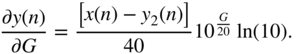
To train the model, a combination of losses is used. The first loss is the mean squared error between the magnitude coefficients given by
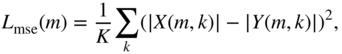
where ![]() and
and ![]() denote the magnitude response vectors of the desired and estimated output signal, respectively, in dB,
denote the magnitude response vectors of the desired and estimated output signal, respectively, in dB, ![]() denotes a frequency bin index,
denotes a frequency bin index, ![]() denotes the frame index, and
denotes the frame index, and ![]() denotes the number of bins. The second loss function is the absolute error between the absolute values of the transformed magnitude response coefficients corresponding to the estimation and ground truth. This loss function is given by
denotes the number of bins. The second loss function is the absolute error between the absolute values of the transformed magnitude response coefficients corresponding to the estimation and ground truth. This loss function is given by

where ![]() denotes the absolute value. This loss function shows an improved noise suppression capability, particularly in unvoiced or silent regions to reduce unpleasant artifacts.
denotes the absolute value. This loss function shows an improved noise suppression capability, particularly in unvoiced or silent regions to reduce unpleasant artifacts.
To train the denoising model, a dataset is built with audio files containing both high fidelity speech and music sampled at ![]() kHz. Short speech files are collected from the PTDB‐TUG [Pir11] dataset, and music files of longer duration are collected from multiple classical music datasets including the Bach10 [Dua10] and Mirex‐Su [Su16] datasets. Two networks are trained with speech and music files, respectively. To train the first network, 200 speech files are selected and some examples from the remaining speech files are selected for testing. The second network is trained with 20 music files while the remaining music files are selected for testing. In this example, a CNN model with eight inception–attention blocks is used for speech denoising and a model with twelve inception–attention blocks for denoising music signals, based on experiments. The models are trained for 70 epochs with adaptive momentum update. The performance of the models can be evaluated by different objective metrics. Improvement in SNR is an indicator of denoising performance, while perceptual evaluation of audio quality (PEAQ) [Thi00] and speech quality (PESQ) [ITU01] are important methods to evaluate audio and speech quality. The PEAQ method provides an objective difference grade (ODG) which rates an audio between
kHz. Short speech files are collected from the PTDB‐TUG [Pir11] dataset, and music files of longer duration are collected from multiple classical music datasets including the Bach10 [Dua10] and Mirex‐Su [Su16] datasets. Two networks are trained with speech and music files, respectively. To train the first network, 200 speech files are selected and some examples from the remaining speech files are selected for testing. The second network is trained with 20 music files while the remaining music files are selected for testing. In this example, a CNN model with eight inception–attention blocks is used for speech denoising and a model with twelve inception–attention blocks for denoising music signals, based on experiments. The models are trained for 70 epochs with adaptive momentum update. The performance of the models can be evaluated by different objective metrics. Improvement in SNR is an indicator of denoising performance, while perceptual evaluation of audio quality (PEAQ) [Thi00] and speech quality (PESQ) [ITU01] are important methods to evaluate audio and speech quality. The PEAQ method provides an objective difference grade (ODG) which rates an audio between ![]() and 0. An ODG score of 0 indicates imperceptible differences compared with the reference and a score of
and 0. An ODG score of 0 indicates imperceptible differences compared with the reference and a score of ![]() indicates an audio with annoying artifacts. Similarly, PESQ provides a mean opinion score (MOS) that ranges from 1, which indicates a poor speech quality, to 5, which indicates an excellent speech quality. The test dataset contains 54 audio files, out of which the first 50 files contain short speech and the remaining files contain music of relatively longer duration. Table 11.1 illustrates the performance of the CNNs for speech and music signals. The average SNR of the denoised speech signals produced by the CNN indicates an improvement of
indicates an audio with annoying artifacts. Similarly, PESQ provides a mean opinion score (MOS) that ranges from 1, which indicates a poor speech quality, to 5, which indicates an excellent speech quality. The test dataset contains 54 audio files, out of which the first 50 files contain short speech and the remaining files contain music of relatively longer duration. Table 11.1 illustrates the performance of the CNNs for speech and music signals. The average SNR of the denoised speech signals produced by the CNN indicates an improvement of ![]() dB. Similarly, the average ODG score of the speech after noise suppression is improved by 0.62. To perform the wideband PESQ evaluation, the speech signals are resampled to
dB. Similarly, the average ODG score of the speech after noise suppression is improved by 0.62. To perform the wideband PESQ evaluation, the speech signals are resampled to ![]() kHz. The average MOS of the denoised signal is nearly improved by 1. The average SNR of the denoised music signals produced by the CNN shows an improvement of approximately
kHz. The average MOS of the denoised signal is nearly improved by 1. The average SNR of the denoised music signals produced by the CNN shows an improvement of approximately ![]() dB. However, the average ODG score of the music signals after noise suppression does not show an improvement similar to that of speech. This indicates that music is relatively more difficult to denoise compared to speech because of a low number of pauses and the presence of more high‐frequency content which gets suppressed along with noise and affects the perceptual quality. Figure 11.17 illustrates an example of denoising on a female speech signal corrupted with noise. The SNR of the denoised speech is
dB. However, the average ODG score of the music signals after noise suppression does not show an improvement similar to that of speech. This indicates that music is relatively more difficult to denoise compared to speech because of a low number of pauses and the presence of more high‐frequency content which gets suppressed along with noise and affects the perceptual quality. Figure 11.17 illustrates an example of denoising on a female speech signal corrupted with noise. The SNR of the denoised speech is ![]() dB, its ODG score is
dB, its ODG score is ![]() compared with a score of
compared with a score of ![]() for the noisy speech, and its MOS score improves from 1.28 to 2.44. Figure 11.18 illustrates an example of denoising on a musical piece from the Mirex‐Su dataset corrupted with noise. The overall improvement in SNR is approximately
for the noisy speech, and its MOS score improves from 1.28 to 2.44. Figure 11.18 illustrates an example of denoising on a musical piece from the Mirex‐Su dataset corrupted with noise. The overall improvement in SNR is approximately ![]() dB, while the ODG score of the denoised signal is
dB, while the ODG score of the denoised signal is ![]() compared with a score of
compared with a score of ![]() for the noisy signal. Figure 11.19 shows the corresponding spectral representations of the noisy, denoised, and original signal.
for the noisy signal. Figure 11.19 shows the corresponding spectral representations of the noisy, denoised, and original signal.
Table 11.1 Average performance of the denoising CNNs on noisy speech and music
| Audio | SNR (dB) | ODG | MOS |
|---|---|---|---|
| Noisy Speech | 5 | 1.48 | |
| Denoised Speech | 18.8 | 2.49 | |
| Noisy Music | 5 | ||
| Denoised Music | 16.3 |
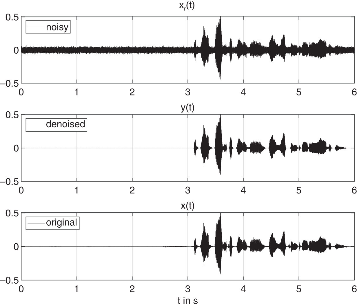
Figure 11.17 Example of noise suppression in an audio file from the PTDB‐TUG speech dataset.

Figure 11.18 Example of noise suppression in an audio file from the Mirex‐Su dataset.
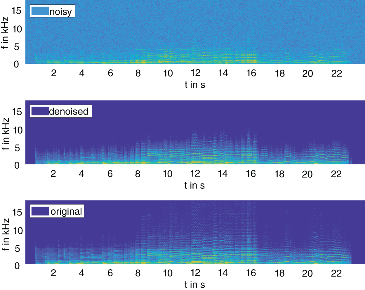
Figure 11.19 Spectrogram of the example noisy, denoised, and original audio file from the Mirex‐Su dataset.
The applications described in this chapter are a few of the many audio processing applications which can be categorized as supervised regression problems. Similar applications with deep learning include audio enhancement in terms of super‐resolution [SD21], supervised audio source separation [LM19], and neural source modeling [Wan20]. Supervised audio classification problems, however, categorize audio signals or inherent features within audio signals into distinct classes which can be used for further processing. Classification problems are also extensively researched and some of the notable applications include pitch detection [SZZ16], music genre classification [Ora17], and speaker recognition [Sny18], among others.
11.5 Exercises
- Write a script for a simple feedforward neural network with an input layer of dimension 1, an output layer of dimension 1, a hidden layer of dimension 5, and an activation and a loss function.
- Train the network with stochastic gradient descent for 50 epochs to fit the function
 , monitor the error, and test the network.
 - Perform the training with a higher number of epochs.
- Perform the training with multiple hidden layers.
- Train the network with stochastic gradient descent for 50 epochs to fit the function
- Replace a fully connected layer with a convolution layer and train the network for the previous example.
- Perform the above exercise and the examples from the chapter using a deep learning toolbox in a framework of your choice (Matlab, Pytorch, Tensorflow).
References
- [Aka12] M. Akamine and J. Ajmera: A decision‐tree‐based algorithm for speech/music classification and segmentation. EURASIP Journal on Audio, Speech, and Music Processing, 10, Feb 2012.
- [Alg01] V. R. Algazi, R. O. Duda, D. M. Thompson, and C. Avendano: The CIPIC HRTF database. Proceedings of the 2001 IEEE Workshop on the Applications of Signal Processing to Audio and Acoustics, pages 99–102, Oct 2001.
- [Bac91] A.D. Back and A. C. Tsoi: FIR and IIR synapses, a new neural network architecture for time series modeling. Neural Computation, 3(3):375–385, 1991.
- [Bah15] D. Bahdanau, K. Cho, and Y. Bengio: Neural machine translation by jointly learning to align and translate. In 3rd International Conference on Learning Representations, May 2015.
- [Bha20] P. Bhattacharya, P. Nowak, and U. Zölzer: Optimization of cascaded parametric peak and shelving filters with backpropagation algorithm. Digital Audio Effects 2020 (DaFX), 2020.
- [Bol79] S. F. Boll: Suppression of acoustic noise in speech using spectral subtraction. IEEE Transactions on Acoustics, Speech, Signal Processing, ASSP‐27(2):113–120, Apr 1979.
- [Chi06] J‐T. Chien and B‐C. Chen: A new independent component analysis for speech recognition and separation. IEEE Transactions on Audio, Speech, and Language Processing, 14(4):1245–1254, 2006.
- [Che16] J. Cheng, L. Dong, and M. Lapata: Long short‐term memory networks for machine reading. In Proceedings of the 2016 Conference on Empirical Methods in Natural Language Processing, pages 551–561, Nov 2016.
- [Car17] H. Caracalla and A. Roebel: Gradient conversion between time and frequency domains using Wirtinger calculus. In Digital Audio Effects 2017 (DaFX), Edinburgh, United Kingdom, Sep 2017.
- [Cam96] P. Campolucci, A. Uncini, and F. Piazza: Fast adaptive IIR‐MLP neural networks for signal processing application. Acoustics, Speech, and Signal Processing, IEEE International Conference on, 6:3529–3532, Jun 1996.
- [Dau15] Y. N. Dauphin, H. de Vries, J. Chung, and Y. Bengio: Rmsprop and equilibrated adaptive learning rates for non‐convex optimization. CoRR, abs/1502.04390, 2015.
- [Duc11] J. Ducji, E. Hazan, and Y. Singer: Adaptive subgradient methods for online learning and stochastic optimization. Journal of Machine Learning Research, 12:2121–2159, Jul 2011.
- [Dua10] Z. Duan, B. Pardo, and C. Zhang: Multiple fundamental frequency estimation by modeling spectral peaks and non‐peak regions. IEEE Trans. Audio Speech Language Process., 18(8):2121–2133, 2010.
- [EM84] Y. Ephra–m and D. Malah: Speech enhancement using a minimum mean‐square error short‐time spectral amplitude estimator. IEEE Transactions on Acoustics, Speech, Signal Processing, ASSP‐ 32(6):1109–1121, Dec 1984.
- [Eng20] J. Engel, L. Hantrakul, C. Gu, and A. Roberts: DDSP: Differentiable Digital Signal Processing. International Conference on Learning Representation, pages 1–19, 2020.
- [Fev09] C. Fevotte, N. Bertin, and J‐L. Durrieu: Nonnegative matrix factorization with the itakura‐saito divergence: With application to music analysis. Neural Computation, 21(3):793–830, 2009.
- [Glo10] X. Glorot and Y. Bengio: Understanding the difficulty of training deep feedforward neural networks. Journal of Machine Learning Research, 9:249–256, 2010.
- [GL03] G. Guodong and S.Z. Li: Content‐based audio classification and retrieval by support vector machines. IEEE Transactions on Neural Networks, 14(1):209–215, 2003.
- [Gao92] F.X.Y. Gao and W.M. Snelgrove: An adaptive backpropagation cascade IIR filter. IEEE Transactions on Circuits and Systems II: Analog and Digital Signal Processing, 39(9):606–610, Sep 1992.
- [God01] S.J. Godsill, P.J. Wolfe, and W.N.W. Fong: Statistical model‐based approaches to audio restoration and analysis. Journal of New Music Research, 30(4):323–338, 2001.
- [Han17] Y. Han, J. Kim, and K. Lee: Deep convolutional neural networks for predominant instrument recognition in polyphonic music. IEEE/ACM Transactions on Audio, Speech, and Language Processing, 25(1):208–221, 2017.
- [Hao19] X. Hao, C. Shan, Y. Xu, S. Sun, and L. Xie: An attention‐based neural network approach for single channel speech enhancement. In ICASSP 2019 ‐ 2019 IEEE International Conference on Acoustics, Speech and Signal Processing, pages 6895–6899, 2019.
- [He15] K. He, X. Zhang, S. Ren, and J. Sun: Delving deep into rectifiers: Surpassing human‐level performance on imagenet classification, 2015.
- [ITU01]ITU Perceptual evaluation of speech quality (PESQ): An objective method for end‐to‐end speech quality assessment of narrow‐band telephone networks and speech codecs, 2001.
- [Kin15] D.P. Kingma and J.Ba. Adam: A method for stochastic optimization. In 3rd International Conference on Learning Representations, ICLR, May 2015.
- [Lav09] Y. Lavner and M.E.P. Davies: A decision‐tree‐based algorithm for speech/music classification and segmentation. EURASIP Journal on Audio, Speech, and Music Processing, 239892, Jun 2009.
- [Ler12] A. Lerch: An introduction to audio content analysis: applications in signal processing and music informatics. John Wiley & Sons, Ltd., 2012.
- [LL01] L. Lu, S.Z. Li, and H‐J. Zhang: Content‐based audio segmentation using support vector machines. In IEEE International Conference on Multimedia and Expo, pages 749–752, 2001.
- [LM19] Y. Luo and N. Mesgarani. Conv‐tasnet: Surpassing ideal timefrequency magnitude masking for speech separation. IEEE/ACM Trans. Audio, Speech and Lang. Proc., 27(8):1256–1266, Aug. 2019.
- [Lu16] Y‐C. Lu, C‐W. Wu, A. Lerch, and C‐T. Lu: Automatic outlier detection in music genre datasets. In Proceedings of the 17th International Society for Music Information Retrieval Conference, ISMIR, pages 101–107, Aug 2016.
- [Mül15] M. Müller: Fundamentals of Music Processing: Audio, Analysis, Algorithms, Applications. Springer Publishing Company, Incorporated, 2015.
- [Mac67] J. MacQueen: Some methods for classification and analysis of multivariate observations. In Proceedings of the 5th Berkeley Symposium on Math, Statistics, and Probability, pages 281–297, 1967.
- [Mar20] M.A.R. Martinez, E. Benetos, and J.D. Reiss: Deep learning for black‐box modeling of audio effects. Applied Sciences, 10(2), 2020.
- [Mee18] H. S. Meet, N. Shah, and A. H. Patil: Time‐frequency masking‐based speech enhancement using generative adversarial network. In 2018 IEEE International Conference on Acoustics, Speech and Signal Processing (ICASSP), pages 5039–5043, 2018.
- [Min19] G. Min, C. Zhang, X. Zhang, and W. Tan: Deep vocoder: Low bit rate compression of speech with deep autoencoder. In 2019 IEEE International Conference on Multimedia Expo Workshops (ICMEW), pages 372–377, 2019.
- [Ner20] S. Nercessian: Neural parametric equalizer matching using differentiable biquads. Digital Audio Effects 2020 (DaFX), 2020.
- [Nes83] Y. Nesterov: A method for unconstrained convex minimization problem with the rate of convergence O(). Doklady ANSSSR, pages 543–547, 1983.
- [Ora17] S. Oramas, O. Nieto, F. Barbieri, and X. Serra: Multi‐label music genre classification from audio, text, and images using deep features. CoRR, abs/1707.04916, 2017.
- [Poh06] T. Pohle, P. Knees, M. Schedl, and G. Widmer: Independent component analysis for music similarity computation. In ISMIR 2006, 7th International Conference on Music Information Retrieval, pages 228–233, Oct 2006.
- [Par17] Se Rim Park and Jin Won Lee: A fully convolutional neural network for speech enhancement. In Proc. Interspeech 2017, pages 1993–1997, 2017.
- [Pir11] G. Pirker, M. Wohlmayr, S. Petrik, and F. Pernkopf: A pitch tracking corpus with evaluation on multipitch tracking scenario. In Interspeech 2011, pages 1509–1512, 2011.
- [Ros61] F. Rosenblatt: Principles of Neurodynamics. Perceptrons and the Theory of Brain Mechanisms. Defense Technical Information Center, 1961.
- [Ros99] R.E. Rose: Training a recursive filter by use of derivative function, US patent US5905659A, May 1999.
- [Ret18] D. Rethage, J. Pons, and X. Serra: A wavenet for speech denoising. In 2018 IEEE International Conference on Acoustics, Speech and Signal Processing (ICASSP), pages 5069–5073, 2018.
- [SD21] S. Sulun and M.E.P. Davies: On filter generalization for music bandwidth extension using deep neural networks. IEEE Journal of Selected Topics in Signal Processing, 15(1):132–142, 2021.
- [Sny17] D. Snyder, D. Garcia‐Romero, D. Povey, and S. Khudanpur: Deep neural network embeddings for text‐independent speaker verification. In Proc. Interspeech 2017, pages 999–1003, 2017.
- [Sny18] D. Snyder, D. Garcia‐Romero, G. Sell, D. Povey, and S. Khudanpur: X‐vectors: Robust dnn embeddings for speaker recognition. In IEEE International Conference on Acoustics, Speech and Signal Processing, pages 5329–5333, 2018.
- [Soo97] I. Y. Soon, S. N. Koh, and C. K Yeo: Wavelet for speech denoising. In Proceedings of IEEE TENCON –97, IEEE Region 10 Annual Conference of Speech and Image Technologies for Computing and Telecommunications, volume 2, pages 479–482, 1997.
- [Sze15] C. Szegedy, L. Wei, J. Yangqing, P. Sermanet, S. Reed, D. Anguelov, D. Erhan, V. Vanhoucke, and A. Rabinovich: Going deeper with convolutions. In 2015 IEEE Conference on Computer Vision and Pattern Recognition, pages 1–9, 2015.
- [Su16] L. Su and Y‐H. Yang: Escaping from the abyss of manual annotation: New methodology of building polyphonic datasets for automatic music transcription. In Music, Mind, and Embodiment, pages 309–321. Springer International Publishing, 2016.
- [SZZ16] H. Su, H. Zhang, X. Zhang, and G. Gao. Convolutional neural network for robust pitch determination. In IEEE International Conference on Acoustics, Speech and Signal Processing, pages 579–583, 2016.
- [Thi00] T. Thiede, W. C. Treurniet, R. Bitto, C. Schmidmer, T. Sporer, J. G. Beerends, and C. Colomes: PEAQ ‐ the ITU standard for objective measurement of perceived audio quality. Journal of the audio engineering society, 48(1/2):3–29, Feb 2000.
- [Tak03] H. Takeshi, M. Takahiro, I. Yoshihisa, and H. Tetsuya: Musical noise reduction using an adaptive filter. Acoustical Society of America Journal, 114(4), Oct 2003.
- [Val18] J‐M. Valin: A hybrid dsp/deep learning approach to real‐time full‐band speech enhancement. In 2018 IEEE 20th International Workshop on Multimedia Signal Processing (MMSP), pages 1–5, 2018.
- [Väl19] V. Välimäki and J. Rämö: Neurally controlled graphic equalizer. IEEE/ACM Transactions on Audio, Speech, and Language Processing, 27(12), Dec 2019.
- [Vir07] T. Virtanen: Monaural sound source separation by nonnegative matrix factorization with temporal continuity and sparseness criteria. IEEE Transactions on Audio, Speech, and Language Processing, 15(3):1066–1074, 2007.
- [Wan20] X. Wang, S. Takaki, and J. Yamagishi: Neural source‐filter waveform models for statistical parametric speech synthesis. IEEE/ACM Transactions on Audio, Speech, and Language Processing, 28:402–415, 2020.
- [Xu15] K. Xu, J. Ba, R. Kiros, K. Cho, A. C. Courville, R. Salakhutdinov, R. S. Zemel, and Y. Bengio: Show, attend and tell: Neural image caption generation with visual attention. In Proceedings of the 32nd International Conference on Machine Learning, volume 37, pages 2048–2057, Jul 2015.
- [Yu08] G. Yu, S. Mallat, and E. Bacry: Audio denoising by time‐frequency block thresholding. IEEE Transactions on Signal Processing, 56(5):1830–1839, 2008.
- [Zha16] J. Zhang, J. Tang, and Li‐R. Dai: RNN‐BLSTM based multi‐pitch estimation. In Interspeech 2016, pages 1785–1789, 2016.